Page 1 :
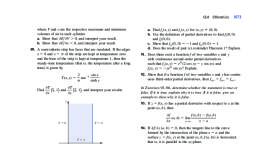
13.4, where V and √ are the respective maximum and minimum, volumes of air in each cylinder., a. Show that E> V  0, and interpret your result., b. Show that E> √  0, and interpret your result., 89. A semi-infinite strip has faces that are insulated. If the edges, x  0 and x  p of the strip are kept at temperature zero, and the base of the strip is kept at temperature 1, then the, steady-state temperature (that is, the temperature after a long, time) is given by, T(x, y) , Find, , T, x, , 1 p2 , 1 2 and, , T, y, , 1073, , a. Find fx(x, y) and fy(x, y) for (x, y)  (0, 0)., b. Use the definition of partial derivatives to find fx(0, 0), and fy(0, 0) ., c. Show that fxy(0, 0)  1 and fyx(0, 0)  1., d. Does the result of part (c) contradict Theorem 1? Explain., 91. Does there exist a function f of two variables x and y, with continuous second-order partial derivatives, such that fx(x, y)  e2x(2 cos xy  y sin xy) and, fy(x, y)  ye2x sin xy? Explain., 92. Show that if a function f of two variables x and y has continuous third-order partial derivatives, then fxyx  fyxx  fxxy., , 2, sin x, tan1, p, sinh y, , 1 p2 , 1 2 , and interpret your results., , y, , In Exercises 93–96, determine whether the statement is true or, false. If it is true, explain why it is true. If it is false, give an, example to show why it is false., 93. If z  f(x, y) has a partial derivative with respect to x at the, point (a, b) , then, , T0, , T0, , π, , x, , 90. Let, xy(x 2  y 2), x 2  y2, 0, , f(x, b)  f(a, b), f, (a, b)  lim, xa, x, x→a, 94. If f> y (a, b)  0, then the tangent line to the curve, formed by the intersection of the plane x  a and the, surface z  f(x, y) at the point (a, b, f(a, b)) is horizontal;, that is, it is parallel to the xy-plane., , T1, 0, , f(x, y)  •, , Differentials, , if (x, y)  (0, 0), if (x, y)  (0, 0), , 95. If fxx(x, y) is defined for all x and y and fxx(a, b)  0 for, all x in the interval (a, b), then the curve C formed by the, intersection of the plane y  b and the surface z  f(x, y), is concave downward on (a, b)., 96. If f(x, y)  ln xy, then fxy(x, y)  fyx(x, y) for all (x, y) in, D  {(x, y) 冟 xy  0}., , 13.4 Differentials, Increments, Recall that if f is a function of one variable defined by y  f(x), then the increment in, y is defined to be, ⌬y  f(x  ⌬x)  f(x), where ⌬x is an increment in x (Figure 1a). The increment of a function of two or more, variables is defined in an analogous manner. For example, if z is a function of two variables defined by z  f(x, y), then the increment in z produced by increments of ⌬x, and ⌬y in the independent variables x and y, respectively, is defined to be, ⌬z  f(x  ⌬x, y  ⌬y)  f(x, y), (See Figure 1b.), , (1)

Page 2 :
1074, , Chapter 13 Functions of Several Variables, z, (x  Δ x, y  Δy, f(x  Δ x, y  Δy)), y  f (x), , y, , z  f (x, y), Δ z  f (x  Δ x, y  Δy)  f(x, y), (x, y, f (x, y)), , (x  Δ x, y  Δy), Δy  f (x  Δ x)  f (x), (x, y), , 0, y, , 0, , x, , x  Δx, , x, x, , (a) The increment Δy is the change in y as x, changes from x to x  Δ x., , (x  Δ x, y  Δy), , (x, y), , (x, y  Δy), , (b) The increment Δ z is the change in z as x, changes from x to x  Δ x and y changes, from y to y  Δy., , FIGURE 1, , EXAMPLE 1 Let z  f(x, y)  2x 2  xy. Find ⌬z. Then use your result to find the, change in z if (x, y) changes from (1, 1) to (0.98, 1.03)., Solution, , Using Equation (1), we obtain, , ⌬z  f(x  ⌬x, y  ⌬y)  f(x, y),  [2(x  ⌬x)2  (x  ⌬x)(y  ⌬y)]  (2x 2  xy),  2x 2  4x ⌬x  2(⌬x)2  xy  x ⌬y  y ⌬x  ⌬x ⌬y  2x 2  xy,  (4x  y) ⌬x  x ⌬y  2(⌬x)2  ⌬x ⌬y, Next, to find the increment in z if (x, y) changes from (1, 1) to (0.98, 1.03), we note, that ⌬x  0.98  1  0.02 and ⌬y  1.03  1  0.03. Therefore, using the result, obtained earlier with x  1, y  1, ⌬x  0.02, and ⌬y  0.03, we obtain, ⌬z  [4(1)  1](0.02)  (1)(0.03)  2(0.02)2  (0.02)(0.03),  0.0886, You can verify the correctness of this result by computing the quantity, f(0.98, 1.03)  f(1, 1)., , The Total Differential, Recall from Section 2.9 that if f is a function of one variable defined by y  f(x), then, the differential of f at x is defined by, dy  f ¿(x) dx, where dx  ⌬x is the differential in x. Furthermore,, ⌬y ⬇ dy, if ⌬x is small (see Figure 2)., , (2)

Page 3 :
13.4, , Differentials, , 1075, , z, (x  Δ x, y  Δy, f (x  Δ x, y  Δy)), y, , y  f (x), , z  f (x, y), dz, , T, dy, , Δz, , Tangent plane, Δy, 0, y, x, , 0, , x, , x  Δx, , (x, y), , x, , (a) Relationship between dy and Δy, , (x  Δ x, y  Δy), , (b) Relationship between dz and Δz. The tangent, plane is the analog of the tangent line T in the, one-variable case., , FIGURE 2, , For an analog of this result for a function of two variables, we begin with the following definition., , DEFINITION Differentials, Let z  f(x, y), and let ⌬x and ⌬y be increments of x and y, respectively. The, differentials dx and dy of the independent variables x and y are, dx  ⌬x, , and, , dy  ⌬y, , The differential dz, or total differential, of the dependent variable z is, dz , , f, f, dx , dy  fx(x, y) dx  fy(x, y) dy, x, y, , Later in this section, we will show that, ⌬z  dz  e1 ⌬x  e2 ⌬y, where e1 and e2 are functions of ⌬x and ⌬y that approach 0 as ⌬x and ⌬y approach 0., This implies that, ⌬z ⬇ dz, , (3), , if both ⌬x and ⌬y are small., Figure 2b shows the geometric relationship between ⌬z and dz. Observe that as x, changes from x to x  ⌬x and y changes from y to y  ⌬y, ⌬z measures the change, in the height of the graph of f, whereas dz measures the change in the height of the, tangent plane.*, , *For now, we will rely on our intuitive definition of the tangent plane. We will define the tangent plane in, Section 13.7.

Page 4 :
1076, , Chapter 13 Functions of Several Variables, , EXAMPLE 2 Let z  f(x, y)  2x 2  xy., a. Find the differential dz., b. Compute the value of dz if (x, y) changes from (1, 1) to (0.98, 1.03) , and compare your result with the value of ⌬z obtained in Example 1., Solution, f, f, dx , dy  (4x  y) dx  x dy, x, y, b. Here x  1, y  1, dx  ⌬x  0.02, and dy  ⌬y  0.03. Therefore,, a. dz , , dz  [4(1)  1](0.02)  1(0.03)  0.09, The value of ⌬z obtained in Example 1 was 0.0886, so dz is a good approximation of ⌬z in this case. Observe that it is easier to compute dz than to compute ⌬z., , EXAMPLE 3 A storage tank has the shape of a right circular cylinder. Suppose that, the radius and height of the tank are measured at 1.5 ft and 5 ft, respectively, with a, possible error of 0.05 ft and 0.1 ft, respectively. Use differentials to estimate the maximum error in calculating the capacity of the tank., Solution The capacity (volume) of the tank is V  pr 2h. The error in calculating the, capacity of the tank is given by, ⌬V ⬇ dV , , V, V, dr , dh  2prh dr  pr 2 dh, r, h, , Since the errors in the measurement of r and h are at most 0.05 ft and 0.1 ft, respectively, we have dr  0.05 and dh  0.1. Therefore, taking r  1.5, h  5, dr  0.05,, and dh  0.1, we obtain, dV  2prh dr  pr 2 dh, ⬇ 2p(1.5)(5)(0.05)  p(1.5)2 (0.1)  0.975p, Thus, the maximum error in calculating the volume of the storage tank is approximately 0.975p, or 3.1, ft3., , EXAMPLE 4 The Error in Computing the Range of a Projectile If a projectile is fired, with an angle of elevation u and initial speed of √ ft/sec, then its range (in feet) is, R, , √2 sin 2u, t, , where t is the constant of acceleration due to gravity. (See Figure 3.) Suppose that a, projectile is launched with an initial speed of 2000 ft/sec at an angle of elevation of, p>12 radians and that the maximum percentage errors in the measurement of √ and u, are 0.5% and 1%, respectively., a. Estimate the maximum error in the computation of the range of the projectile., b. Find the maximum percentage error in computing the range of this projectile.

Page 5 :
13.4, , FIGURE 3, We want to find the range R of a, projectile fired with an angle of, elevation u and initial speed of √ ft/sec., , Differentials, , 1077, , q, R, , Solution, a. The error in the computation of R is, ⌬R ⬇ dR , , R, R, 2√ sin 2u, 2√2 cos 2u, d√ , du , d√ , du, t, t, √, u, , The maximum error in the computation of √ is (0.005)(2000) or 10 ft/sec; that is,, 冟 d√ 冟 10. Also, the maximum error in the computation of u is (0.01)(p>12) radians. In other words, 冟 du 冟 0.01(p>12). Therefore, the maximum error in computing the range of the projectile is approximately, 冟 ⌬R 冟 ⬇ 冟 dR 冟, , 2√2 cos 2u, 2√ sin 2u, 冟 d√ 冟 , 冟 du 冟, t, t, , p, p, 2(2000) sin a b, 2(2000)2 cos a b, 6, 6, 0.01p, , (10) , a, b, 32, 32, 12, ⬇ 1192, or approximately 1192 ft., b. Using √  2000 and u  p>12, we find the range of the projectile to be, p, (2000)2 sin a b, 6, √ sin 2u, R, ,  62,500, t, 32, 2, , Therefore, the maximum percentage error in computing the range of the projectile is, 100 `, , ⌬R, 1192, ` ⬇ 100a, b, R, 62,500, , or approximately 1.91%., , Error in Approximating ⌬z by dz, The following theorem tells us that dz gives a good approximation of ⌬z if ⌬x and ⌬y, are small, provided that both fx and fy are continuous., , THEOREM 1, Let f be a function defined on an open region R. Suppose that the points (x, y), and (x  ⌬x, y  ⌬y) are in R and that fx and fy are continuous at (x, y). Then, ⌬z  fx(x, y) ⌬x  fy(x, y) ⌬y  e1 ⌬x  e2 ⌬y, where e1 and e2 are functions of ⌬x and ⌬y such that, lim, , (⌬x, ⌬y)→(0, 0), , e1  0, , and, , lim, , (⌬x, ⌬y)→(0, 0), , e2  0

Page 6 :
1078, , Chapter 13 Functions of Several Variables, , PROOF Fix x and y. By adding and subtracting f(x  ⌬x, y) to ⌬z, we have, ⌬z  f(x  ⌬x, y  ⌬y)  f(x, y),  [ f(x  ⌬x, y)  f(x, y)]  [ f(x  ⌬x, y  ⌬y)  f(x  ⌬x, y)],  ⌬z 1  ⌬z 2, where ⌬z 1 is the change in z as (x, y) changes from (x, y) to (x  ⌬x, y) and ⌬z 2 is the, change in z as (x, y) changes from (x  ⌬x, y) to (x  ⌬x, y  ⌬y). (See Figure 4a.), z, (x  Δ x, y  Δy, f(x  Δ x, y  Δy)), (x  Δ x, y, f(x  Δ x, y)), y, Δ z2, C(x  Δ x, y  Δy), , (x, y, f(x, y)), , Δ z1, , 0, A(x, y), x, , FIGURE 4, , B(x  Δ x, y), , (x  Δ x, y1), A(x, y) (x1, y), , y, C(x  Δ x, y  Δy), , (a) Δ z1  f (x  Δ x, y)  f (x, y) and, Δ z2  f (x  Δ x, y  Δy)  f(x  Δ x, y), , B(x  Δ x, y), , 0, , x, , (b) The points A, B, and C shown in the, xy-plane., , On the interval between A and B, y is constant, so the function t defined by, t(t)  f(t, y) for x t x  ⌬x is a function of one variable. (See Figure 4b.) Therefore, by the Mean Value Theorem, there exists a point (x 1, y) with x  x 1  x  ⌬x, such that, t(x  ⌬x)  t(x)  t¿(x 1) ⌬x, Since t¿(x 1)  fx(x 1, y) , we have, ⌬z 1  f(x  ⌬x, y)  f(x, y)  t(x  ⌬x)  t(x),  t¿(x 1) ⌬x  fx(x 1, y) ⌬x, , x  x 1  x  ⌬x, , Next, on the interval between B and C, both x and ⌬x are constant, so the function, h defined by h(t)  f(x  ⌬x, t) for y t y  ⌬y is a function of one variable. (See, Figure 4b.) Therefore, by the Mean Value Theorem there exists a point (x  ⌬x, y1), with y  y1  y  ⌬y such that, h(y  ⌬y)  h(y)  h¿(y1) ⌬y, Since h¿(y1)  fy(x  ⌬x, y1) , we have, ⌬z 2  f(x  ⌬x, y  ⌬y)  f(x  ⌬x, y),  h(y  ⌬y)  h(y)  h¿(y1) ⌬y  fy(x  ⌬x, y1) ⌬y, Therefore,, ⌬z  ⌬z 1  ⌬z 2,  fx(x 1, y) ⌬x  fy(x  ⌬x, y1) ⌬y

Page 7 :
13.4, , Differentials, , 1079, , Adding and subtracting fx(x, y) ⌬x  fy(x, y) ⌬y to the right-hand side of the previous, equation and rearranging terms, we obtain, ⌬z  fx(x, y) ⌬x  fy(x, y) ⌬y  [ fx(x 1, y)  fx(x, y)] ⌬x  [ fy(x  ⌬x, y1)  fy(x, y)] ⌬y,  fx(x, y) ⌬x  fy(x, y) ⌬y  e1 ⌬x  e2 ⌬y, where, e1  fx(x 1, y)  fx(x, y), and, e2  fy(x  ⌬x, y1)  fy(x, y), Observe that as (⌬x, ⌬y) → (0, 0), x 1 → x and y1 → y. Therefore, the continuity of fx, and fy implies that, lim, , (⌬x, ⌬y)→(0, 0), , e1  0, , and, , lim, , (⌬x, ⌬y)→(0, 0), , e2  0, , and this proves the result., Note, , Observe that the conclusion of Theorem 1 can be written as, ⌬z  dz  e1 ⌬x  e2 ⌬y, , Therefore, if ⌬x and ⌬y are both small, then, ⌬z  dz  (small number)(small number)  (small number)(small number), and this quantity is a very small number, which accounts for the closeness of the, approximation. Compare this with the case of a function of one variable discussed in, Section 2.9., , Differentiability of a Function of Two Variables, The conclusion of Theorem 1 can be written as, ⌬z  dz  e1 ⌬x  e2 ⌬y, , (4), , where e1 → 0 and e2 → 0 as (⌬x, ⌬y) → (0, 0). We define a function of two variables, to be differentiable if z  f(x, y) satisfies Equation (4)., , DEFINITION Differentiability of a Function of Two Variables, Let z  f(x, y). The function f is differentiable at (a, b) if ⌬z can be expressed, in the form, ⌬z  fx(a, b) ⌬x  fy(a, b) ⌬y  e1 ⌬x  e2 ⌬y, where e1 → 0 and e2 → 0 as (⌬x, ⌬y) → (0, 0). The function f is differentiable, in a region R if it is differentiable at each point of R., , EXAMPLE 5 Show that the function f defined by f(x, y)  2x 2  xy is differentiable, in the plane., Solution Write z  f(x, y)  2x 2  xy, and let (x, y) be any point in the plane. Then, using the result of Example 1, we have, ⌬z  (4x  y) ⌬x  x ⌬y  2(⌬x)2  ⌬x ⌬y

Page 8 :
1080, , Chapter 13 Functions of Several Variables, , Since fx  4x  y and fy  x, we can write, ⌬z  fx ⌬x  fy ⌬y  e1 ⌬x  e2 ⌬y, where e1  2 ⌬x and e2  ⌬x. Since e1 → 0 and e2 → 0 as (⌬x, ⌬y) → (0, 0), it follows that f is differentiable at (x, y). But (x, y) is any point in the plane, so f is differentiable in the plane., The next theorem, which is an immediate consequence of Theorem 1, guarantees, when a function of two variables is differentiable., , THEOREM 2 Criterion for Differentiability, Let f be a function of the variables x and y. If fx and fy exist and are continuous, on an open region R, then f is differentiable in R., , For the function f(x, y)  2x 2  xy of Example 5, we have fx(x, y)  4x  y and, fy(x, y)  x, both of which are continuous everywhere. Therefore, by Theorem 2 we, conclude that f is differentiable in the plane, as demonstrated earlier., , !, , Remember that the mere existence of the partial derivatives fx and fy of a function, f at a point (x, y) is not enough to guarantee the differentiability of f at (x, y). (See, Exercise 43.), , Differentiability and Continuity, Just as a differentiable function of one variable is continuous, the following theorem, shows that a differentiable function of two variables is also continuous., , THEOREM 3 Differentiable Functions Are Continuous, Let f be a function of two variables. If f is differentiable at (a, b) , then f is continuous at (a, b)., , PROOF Using the result of Theorem 1, we have, ⌬z  f(a  ⌬x, b  ⌬y)  f(a, b),  fx(a, b) ⌬x  fy(a, b) ⌬y  e1 ⌬x  e2 ⌬y, Writing x  a  ⌬x and y  b  ⌬y, we have, f(x, y)  f(a, b)  [ fx(a, b)  e1](x  a)  [ fy(a, b)  e2](y  b), Noting that e1 → 0 and e2 → 0 as (⌬x, ⌬y) → (0, 0), we see that, f(x, y)  f(a, b) → 0 as, , (⌬x, ⌬y) → (0, 0), , Equivalently,, lim, , (x, y)→(a, b), , Therefore, f is continuous at (a, b) ., , f(x, y)  f(a, b)

Page 9 :
13.4, , Differentials, , 1081, , Functions of Three or More Variables, The notions of differentiability and the differential of functions of more than two variables are similar to those of functions of two variables. For example, suppose that f is, a function of three variables that is defined by w  f(x, y, z). Then the increment ⌬w, of w corresponding to increments of ⌬x, ⌬y, and ⌬z of x, y, and z, respectively, is, ⌬w  f(x  ⌬x, y  ⌬y, z  ⌬z)  f(x, y, z), The function f is differentiable at (x, y, z) if ⌬w can be written in the form, ⌬w  fx(x, y, z) ⌬x  fy(x, y, z) ⌬y  fz(x, y, z) ⌬z  e1 ⌬x  e2 ⌬y  e3 ⌬z, where e1, e2, and e3 are functions of ⌬x, ⌬y, and ⌬z that approach zero as, (⌬x, ⌬y, ⌬z) → (0, 0, 0)., The differential dw of the dependent variable w is defined to be, dw , , w, w, w, dx , dy , dz, x, y, z, , where dx  ⌬x, dy  ⌬y, and dz  ⌬z are the differentials of the independent variables, x, y, and z. If f has continuous partial derivatives and dx, dy, and dz are all small,, then ⌬w ⬇ dw., , EXAMPLE 6 Maximum Error in Calculating Centrifugal Force A centrifuge is a, machine designed for the specific purpose of subjecting materials to a sustained centrifugal force. The magnitude of a centrifugal force F in dynes is given by, F  f(M, S, R) , , p2S 2MR, 900, , where S is in revolutions per minute (rpm), M is the mass in grams, and R is the radius, in centimeters. If the maximum percentage errors in the measurement of M, S, and R, are 0.1%, 0.4%, and 0.2%, respectively, use differentials to estimate the maximum percentage error in calculating F., Solution, , The error in calculating F is ⌬F, and, ⌬F ⬇ dF , , , F, F, F, dM , dS , dR, M, S, R, p2S 2R, 2p2SMR, p2S 2M, dM , dS , dR, 900, 900, 900, , Therefore,, ⌬F, dF, dM, dS, dR, ⬇, , 2, , F, F, M, S, R, and, `, , ⌬F, dF, `⬇`, `, F, F, , `, , dM, dS, dR, `  2` `  `, `, M, S, R, , Since, `, , dM, `, M, , 0.001,, , `, , dS, `, S, , 0.004,, , and, , `, , dR, `, R, , 0.002

Page 10 :
1082, , Chapter 13 Functions of Several Variables, , we have, `, , dF, `, F, , 0.001  2(0.004)  0.002  0.011, , Thus, the maximum percentage error in calculating the centrifugal force is approximately 1.1%., , 13.4, , CONCEPT QUESTIONS, , 1. If z  f(x, y), what is the differential of x? The differential, of y? What is the total differential of z?, 2. Let z  f(x, y). What is the relationship between the actual, change ⌬z, when x changes from x to x  ⌬x and y changes, from y to y  ⌬y, and the total differential dz of f at (x, y)?, 3. a. What does it mean for a function f of two variables x and, y to be differentiable at (a, b)? To be differentiable in a, region R?, , 13.4, , EXERCISES, , 1. Let z  2x 2  3y 2, and suppose that (x, y) changes from, (2, 1) to (2.01, 0.98)., a. Compute ⌬z., b. Compute dz., c. Compare the values of ⌬z and dz., 2. Let z  x  2xy  3y , and suppose that (x, y) changes, from (2, 1) to (1.97, 1.02) ., a. Compute ⌬z., b. Compute dz., c. Compare the values of ⌬z and dz., 2, , 2, , In Exercises 3–20, find the differential of the function., 4. z  x 4  2x 2y 2  3xy 2  y 3, , 3. z  3x 2y 3, 5. z , , xy, xy, , 6. w , , 7. z  (2x 2y  3y 3)3, 9. w  ye, , b. Give a condition that guarantees that a function f of two, variables x and y is differentiable in an open region R., c. If a function f of two variables x and y is differentiable, at (a, b), what can you say about the continuity of f at, (a, b)?, , x2 y2, , xy, 1x, , 2, , 8. z  22x 2  3y 2, 10. z  ln(2x  3y), , 11. w  x ln(x  y ), , 12. z  x 2 sin 2y, , 13. z  e2x cos 3y, , y, 14. w  tan1 a b, x, , 15. w  x 2  xy  z 2, , 16. w  2x 2  xy  z 2, , 17. w  x 2eyz, , 18. w  ex sin(2y  3z), , 19. w  x 2ey  y ln z, , 20. w  x cosh yz, , 2, , 2, , 2, , 2, , x, 22. f(x, y)  12x  3y  ;, y, (2.96, 1.02) ., , 23. f(x, y, z)  ln(2x  y)  e2xz;, (2, 3, 0) to (2.01, 2.97, 0.04)., 24. f(x, y, z)  x 2y cos pz;, (0.98, 2.97, 2.01)., , (x, y, z) changes from, , (x, y, z) changes from (1, 3, 2) to, , 25. The dimensions of a closed rectangular box are measured as, 30 in., 40 in., and 60 in., with a maximum error of 0.2 in. in, each measurement. Use differentials to estimate the maximum error in calculating the volume of the box., 26. Use differentials to estimate the maximum error in calculating the surface area of the box of Exercise 25., 27. A piece of land is triangular in shape. Two of its sides are, measured as 80 and 100 ft, and the included angle is measured as p>3 rad. If the sides are measured with a maximum, error of 0.3 ft and the angle is measured with a maximum, error of p>180 rad, what is the approximate maximum error, in the calculated area of the land?, 28. Production Functions The productivity of a certain country is, given by the function, f(x, y)  30x 4>5y 1>5, when x units of labor and y units of capital are utilized., What is the approximate change in the number of units produced if the amount expended on labor is decreased from, 243 to 240 units and the amount expended on capital is, increased from 32 units to 35 units?, , In Exercises 21–24, use differentials to approximate the, change in f due to the indicated change in the independent, variables., 21. f(x, y)  x 4  3x 2y 2  y 3  2y  4;, (2, 2) to (1.98, 2.01) ., , (x, y) changes from (3, 1) to, , (x, y) changes from, , 29. The pressure P (in pascals), the volume V (in liters), and the, temperature T (in kelvins) of an ideal gas are related by the, , V Videos for selected exercises are available online at www.academic.cengage.com/login.

Page 11 :
13.4, equation PV  8.314T. Use differentials to find the approximate change in the pressure of the gas if its volume increases from 20 L to 20.2 L and its temperature decreases, from 300 K to 295 K., 30. Consider the ideal gas law equation PV  8.314T of Exercise 29. If T and P are measured with maximum errors of, 0.6% and 0.4%, respectively, determine the maximum percentage error in calculating the value of V., 31. Surface Area of Humans The surface area S of humans is, related to their weight W and height H by the formula, S  0.1091W 0.425H 0.725. If W and H are measured with maximum errors of 3% and 2%, respectively, find the approximate maximum percentage error in the measurement of S., 32. Specific Gravity The specific gravity of an object with density, greater than that of water can be determined by using the, formula, S, , A, AW, , where A and W are the weights of the object in air and in, water, respectively. If the measurements of an object are, A  2.2 lb and W  1.8 lb with maximum errors of 0.02 lb, and 0.04 lb, respectively, find the approximate maximum, error in calculating S., , pPR 4, 8kL, , where L is the length of the arteriole in centimeters, R is the, radius in centimeters, P is the difference in pressure between, the two ends of the arteriole in dyne-sec/cm2, and k is the, viscosity of blood in dyne-sec/cm2. Find the approximate, maximum percentage error in measuring the flow of blood if, an error of at most 1% is made in measuring the length of, the arteriole and an error of at most 2% is made in measuring its radius. Assume that P and k are constant., 34. The figure below shows two long, parallel wires that are at, a distance of d m apart, carrying currents of I1 and I2 amps., It can be shown that the force of attraction per unit length, between the two wires as a result of magnetic fields generated by the currents is given by, f, , 36. Error in Calculating the Power of a Battery Suppose the source, of current in an electric circuit is a battery. Then the power, output P (in watts) obtained if the circuit has a resistance, of R ohms is given by, P, , E 2R, (R  r)2, , where E is the electromotive force (EMF) in volts and r is the, internal resistance of the battery. Estimate the maximum percentage error in calculating the power if an EMF of 12 volts, is applied in a circuit with a resistance of 100 ohms, the internal resistance of the battery is 5 ohms, and the possible maximum percentage errors in measuring E, R, and r are 2%, 3%,, and 1%, respectively., 37. Error in Measuring the Resistance of a Circuit The total resistance, R (in ohms) of three resistors with resistances of R1, R2, and, R3 ohms connected in parallel is given by, 1, 1, 1, 1, , , , R, R1, R2, R3, If R1, R2, and R3 are measured as 20, 30, and 50 ohms,, respectively, with a maximum error of 0.5 in each measurement, estimate the maximum error in the calculated value, of R., 38. A container with a constant cross section of A ft2 is filled, with water to a height of h ft. The water is then allowed to, flow out through an orifice of cross section a in.2 located at, the base of the container. It can be shown that the time (in, seconds) that it takes to empty the tank is given by, T  f(A, a, h) , , A 2h, aB t, , where t is the constant of acceleration. Suppose that the, measurements of A, a, and h are 5 ft2, 2 in.2, and 16 ft with, errors of 0.05 ft2, 0.04 in.2, and 0.2 ft, respectively. Find, the error in computing T. (Take t to be 32 ft/sec2.), , m0 I1I2, a, b, 2p D, , A ft 2, , teslas per meter, where m0 (4p 107 N/amp2) is a constant called the permeability of free space. Use differentials, to find the approximate percentage change in f if I1 increases, by 2%, I2 decreases by 2%, and D decreases by 5%., , h ft, , I1, d, I2, , 1083, , 35. Error in Measuring the Period of a Pendulum The period T of a, simple pendulum executing small oscillations is given by, T  2p2L>t, where L is the length of the pendulum and t, is the constant of acceleration due to gravity. If T is computed by using L  4 ft and t  32 ft/sec2, find the approximate percentage error in T if the true values for L and t are, 4.05 ft and 32.2 ft/sec2., , 33. Flow of Blood The flow of blood through an arteriole measured in cm3/sec is given by, F, , Differentials, , a in.2

Page 12 :
1084, , Chapter 13 Functions of Several Variables, , 39. Suspension Bridge Cables The supports of a cable of a suspension bridge are at the same level and at a distance of L ft, apart. The supports are a feet higher than the lowest point of, the cable (see the figure). If the weight of the cable is negligible and the bridge has a uniform weight of W lb/ft, then, the tension (in lb) in the cable at its lowest point is given by, H, , WL2, 8a, , that is located 400 ft above the target. If the initial speed of, the projectile, the angle of elevation of the cannon, and the, height of the site above the target are measured with maximum possible percentage errors of 0.05%, 0.02%, and 0.5%,, respectively, find the maximum error in computing the time, of flight of the projectile. (Take t to be 32 ft/sec2.), In Exercises 41 and 42, show that the function is differentiable, in the plane. (See Example 5.), , If W, L, and a are measured with possible maximum errors, of 1%, 2%, and 2%, respectively, determine the maximum, percentage error in calculating H., , 41. f(x, y)  x 2  y 2, 42. f(x, y)  2xy  y 2, 43. Let f be defined by, , a, , xy, , f(x, y)  • x 2  y 2, 0, , if (x, y)  0, if (x, y)  (0, 0), , Show that fx(0, 0) and fy(0, 0) both exist but that f is not differentiable at (0, 0)., , L, , Hint: Use the result of Theorem 3., , 40. Flight of a Projectile A projectile is fired with a muzzle velocity of √ ft/sec at an angle a radians above the horizontal. If, the launch site is located at a height of h ft above the target, (see the figure below), then the time of the flight of the projectile in seconds is given by, √ sin a  2(√ sin a)  2th, 2, , T, , t, , In Exercises 44–47, determine whether the statement is true or, false. If it is true, explain why it is true. If it is false, give an, example to show why it is false., 44. If z  f(x, y) and dz  0 for all x and y and for all differentials dx and dy, then fx(x, y)  0 and fy(x, y)  0 for all x, and y., 45. If f(x, y) is differentiable at (a, b) , then, f(a, b)  lim (x, y)→(a, b) f(x, y)., 46. If F(x, y)  f(x)  t(y), where f and t are differentiable, in the interval (a, b), then F is differentiable on, R  {(x, y) 冟 a  x  b, a  y  b}., 47. The function, , h, , x 2  y2, 1, is differentiable everywhere., f(x, y)  e, , Suppose that the projectile is fired with an initial speed of, 800 ft/sec at an angle of elevation of p>4 radians from a site, , if (x, y)  (0, 0), if (x, y)  (0, 0), , 13.5 The Chain Rule, The Chain Rule for Functions Involving One Independent Variable, dy, dx, y, , dx, dt, x, dy, dy dx, , dt, dx dt, , FIGURE 1, To find dy>dt, compute dy>dx, ( y depends on x), compute dx>dt, (x depends on t), and then multiply, the two quantities together., , t, , In this section we extend the Chain Rule to functions of two or more variables. First,, let’s recall the Chain Rule for functions of one variable: If y is a differentiable function of x and x is a differentiable function of t (so that y is a function of t), then, dy dx, dy, , dt, dx dt, This rule is easily recalled by using the diagram shown in Figure 1., We begin by looking at the Chain Rule for the case in which a variable w depends, on two intermediate variables x and y, which in turn depend on a third variable t (so, w is a function of one independent variable t).

Page 13 :
13.5, , The Chain Rule, , 1085, , THEOREM 1 The Chain Rule for Functions Involving, One Independent Variable, Let w  f(x, y), where f is a differentiable function of x and y. If x  t(t) and, y  h(t), where t and h are differentiable functions of t, then w is a differentiable function of t, and, dw, w dx, w dy, , , dt, x dt, y dt, , Note Observe that the derivative of w with respect to t is written with an ordinary d, (d) rather than a curly d ( ), since w is a function of the single variable t., , PROOF Let t change from t to t  ⌬t. This produces a change, ⌬x  t(t  ⌬t)  t(t), in x from x to x  ⌬x and a change, ⌬y  h(t  ⌬t)  h(t), in y from y to y  ⌬y. Since t and h are differentiable, they are continuous at t, so, both ⌬x and ⌬y approach zero as ⌬t approaches zero., Next, observe that the changes of ⌬x in x and ⌬y in y in turn produce a change ⌬w, in w from w to w  ⌬w. Since f is differentiable, we have, ⌬w , , w, w, ⌬x , ⌬y  e1 ⌬x  e2 ⌬y, x, y, , where e1 → 0 and e2 → 0 as (⌬x, ⌬y) → (0, 0). Dividing both sides of this equation, by ⌬t, we have, ⌬y, ⌬w, w ⌬x, w ⌬y, ⌬x, , ,  e1,  e2, ⌬t, x ⌬t, y ⌬t, ⌬t, ⌬t, Letting ⌬t → 0, we have, dw, ⌬w,  lim, dt, ⌬t→0 ⌬t, , , ⌬y, ⌬y, w, ⌬x, w, ⌬x, lim, , lim,  lim e1 lim,  lim e2 lim, x ⌬t→0 ⌬t, y ⌬t→0 ⌬t, ⌬t→0, ⌬t→0 ⌬t, ⌬t→0, ⌬t→0 ⌬t, , , , dy, w dx, w dy, dx, , 0ⴢ, 0ⴢ, x dt, y dt, dt, dt, , , , w dx, w dy, , x dt, y dt, , The tree diagram in Figure 2 will help you recall this version of the Chain Rule., There are two “limbs” on this tree leading from w to t. To find dw>dt, multiply the partial derivatives along each limb, and then add the products of these partial derivatives., ∂w, ∂x, , x, , dx, dt, , w, , FIGURE 2, w depends on t via x and y., , t, ∂w, ∂y, , y, , dy, dt

Page 14 :
Chapter 13 Functions of Several Variables, , EXAMPLE 1 Let w  x 2y  xy 3, where x  cos t and y  et. Find dw>dt and its, , value when t  0., , Solution Observe that w is a function of x and y and that both these variables are, functions of t. Thus, we have the situation depicted in the schematic in Figure 2. Using, the Chain Rule, we have, dw, w dx, w dy, , , dt, x dt, y dt,  (2xy  y 3)(sin t)  (x 2  3xy 2)et,  y(y 2  2x)sin t  x(x  3y 2)et, To find the value of dw>dt when t  0, we first observe that if t  0, then x  cos 0  1, and y  e0  1. So, dw, `,  0  1(1  3)e0  2, dt t0, The Chain Rule in Theorem 1 can be extended to the case involving a function of, any finite number of intermediate variables. For example, if w  f(x 1, x 2, p , x n) , where, f is a differentiable function of x 1, x 2, p , x n and x 1  f1(t), x 2  f2(t), p , x n  fn (t),, where f1, f2, p , fn are differentiable functions of t, then, dw, w dx 1, w dx 2, w dx n, , ,  p , dt, x 1 dt, x 2 dt, x n dt, This is easier to recall if you look at Figure 3, which shows the dependency of the variables involved: Multiply the derivatives along each limb leading from w to t, and add, the products of these derivatives., , ∂w, ∂x1, , FIGURE 3, w depends on t via x 1, x 2, p , x n., , ∂w, ∂x2 x, 2, , dx2, dt, , ..., , ..., , w, , x1, , dx1, dt, , ∂w, ∂xn, , t, , ..., , 1086, , xn, , dxn, dt, , EXAMPLE 2 Tracking a Missile Cruiser Figure 4 depicts an AWACS (Airborne Warning and Control System) aircraft tracking a missile cruiser. The flight path of the plane, is described by the parametric equations, x  20 cos 12t,, , y  20 sin 12t,, , z3, , and the course of the missile cruiser is given by, x  30  20t,, , y  40  10t 2,, , z0, , where 0 t 1, and x, y, and z are measured in miles and t in hours. How fast is the, distance between the AWACS plane and the missile cruiser changing when t  0?

Page 16 :
1088, , Chapter 13 Functions of Several Variables, , Therefore, when t  0,, dD,  (0.24)(0)  (0.24)(20)  (0.97)(240)  (0.97)(0), dt,  228, that is, the distance between the AWACS aircraft and the missile cruiser is decreasing, at the rate of 228 mph at that instant of time., , The Chain Rule for Functions Involving Two Independent Variables, We now look at the Chain Rule for the case in which a variable w depends on two, intermediate variables x and y, each of which in turn depends on two variables u and, √ (so that w is a function of two independent variables u and √). More specifically, we, have the following theorem., , THEOREM 2 The Chain Rule for Functions Involving, Two Independent Variables, Let w  f(x, y), where f is a differentiable function of x and y. Suppose that, x  t(u, √) and y  h(u, √) and the partial derivatives t> u, t> √, h> u, and, h> √ exist. Then, , ∂w, ∂x, , ∂x, ∂u, , u, , ∂x, ∂√, , √, , ∂y, ∂u, , u, , w, w x, w y, , , u, x u, y u, and, , x, , w, w x, w y, , , √, x √, y √, , w, ∂w, ∂y, , PROOF For w> u we think of √ as a constant, so t and h are differentiable functions, , y, ∂y, ∂√, , √, , FIGURE 6, w depends on u and √ via x and y., , of u. Then the result follows from Theorem 1. The expression w> √ is derived in a, similar manner., The tree diagram shown in Figure 6 will help you to recall the Chain Rule given, in Theorem 2., To obtain w> u, observe that w is connected to u by two “limbs,” one from w to, u via x and the other from w to u via y. Multiply the partial derivatives along each of, these limbs, and add the product of these partial derivatives together to get w> u. The, expression for w> √ is found in a similar manner., , EXAMPLE 3 Let w  2x 2y, where x  u 2  √2 and y  u 2  √2. Find w> u and, w> √., Solution Observe that w is a function of x and y and that both of these variables are, functions of u and √. Thus, we have the situation depicted in Figure 6. Using the Chain, Rule (Theorem 2), we have, w x, w y, w, , , u, x u, y u,  4xy(2u)  2x 2 (2u)  4xu(2y  x)

Page 17 :
13.5, , The Chain Rule, , 1089, , and, w, w x, w y, , , √, x √, y √,  4xy(2√)  2x 2(2√)  4x√(2y  x), , The General Chain Rule, The Chain Rule in Theorem 2 can be extended to the case involving any finite, number of intermediate variables and any finite number of independent variables., For example, if w  f(x 1, x 2, p , x n) , where f is a differentiable function of n intermediate variables, x 1, x 2, p , x n, and x 1  f1 (t 1, t 2, p , t m) , x 2  f2 (t 1, t 2, p , t m), p ,, x n  fn (t 1, t 2, p , t m) , where f1, f2, p , fn are differentiable functions of m variables,, t 1, t 2, p , t m, then, w, w x1, w x2 p, w xn, , ,  , t1, x 1 t1, x 2 t1, x n t1, w, w x1, w x2 p, w xn, , ,  , t2, x 1 t2, x 2 t2, x n t2, o, w, w x1, w x2 p, w xn, , ,  , tm, x 1 tm, x 2 tm, x n tm, (See Figure 7.), , ∂w, ∂x1, ∂w, ∂x2, , x1, , ∂x1 t1, ∂t2, t2, ∂x1, ∂tm, tm, t1, ..., , ∂x1, ∂t1, , x2, , ..., , ∂w, ∂xn, , ..., , t2, , w, , tm, t1, t2, ..., , xn, , tm, , FIGURE 7, w depends on t 1, t 2, p , t m via x 1, x 2, p , x n., , EXAMPLE 4 Let w  x 2y  y 2z 3, where x  r cos s, y  r sin s, and z  res. Find, , the value of w> s when r  1 and s  0., , Solution Observe that w is a function of x, y, and z, which in turn are functions of r, and s (Figure 8).

Page 18 :
1090, , Chapter 13 Functions of Several Variables, ∂x, ∂r, ∂w, ∂x, , w, , ∂w, ∂y, , r, , Multiplying the partial derivatives on the limbs that connect w to s on the tree diagram, and adding the products of these derivatives, we obtain, , ∂x, ∂s, , x, , s, , ∂y, ∂r, , ∂w, ∂z, , When r  1 and s  0, we have x  1, y  0, and z  1, so, w,  2(1)(0)(0)  (1)(1)  3(0)(1)(1)  1, s, , s, , ∂z, ∂r, , r, , ∂z, ∂s, , z, ,  2xy(r sin s)  (x 2  2yz 3)(r cos s)  3y 2z 2(res), , r, , ∂y, ∂s, , y, , w, w x, w y, w z, , , , s, x s, y s, z s, , EXAMPLE 5 If w  f(x 2  y 2, y 2  x 2) and f is differentiable, show that w satisfies, s, , the equation, , FIGURE 8, w depends on r and s via x, y, and z., x, u, , y, , w, w, x, 0, x, y, , Solution Introduce the intermediate variables u  x 2  y 2 and √  y 2  x 2. Then, w  t(x, y)  f(u, √) (Figure 9)., Using the Chain Rule, we have, , y, , w, w u, w √, w, w, , , , (2x) , (2x), x, u x, √ x, u, √, , w, x, , and, , √, , w, w u, w √, w, w, , , , (2y) , (2y), y, u y, √ y, u, √, , y, , FIGURE 9, w depends on x and y via the, intermediate variables u and √., , Therefore,, y, , r, , EXAMPLE 6 Let w  f(x, y), where f has continuous second-order partial derivatives, and let x  r 2  s 2 and y  2rs. Find 2w> r 2., Solution, , x, s, w, , w, w, w, w, w, w, x,  a2xy,  2xy, b  a2xy,  2xy, b0, x, y, u, √, u, √, , We begin by calculating w> r. Using the Chain Rule, we have, w, w x, w y, w, w, , , , (2r) , (2s), r, x r, y r, x, y, , r, , (See Figure 10.) Next, we apply the Product Rule to w> r to obtain, y, , 2, , w, , s, , FIGURE 10, w depends on r and s via the, intermediate variables x and y., , r, , 2, , , 2, , r, , a2r, , w, w,  2s, b, x, y, , w, w, w,  2r, a b  2s, a b, x, r, x, r, y, , (1), , To compute the partial derivatives appearing in the last two terms of Equation (1), we, observe that since w is a function of r and s via the intermediate variables x and y, the, same is true of w> x and w> y (Figure 11).

Page 19 :
13.5, r, s, , r, , r, , a, , y, w, w, x, w, b, a b, , a b, x, x, x, r, y, x, r, 2, , y, , , , s, , w, , x, , 2, , 2, , w, (2s), y x, , (2r) , , and, , r, x, s, , ∂w, ∂y, , 1091, , Using the Chain Rule once again, we have, , x, ∂w, ∂x, , The Chain Rule, , r, , r, , a, , y, w, w, x, w, b, a b, , a b, y, x, y, r, y, y, r, 2, , , , y, s, , FIGURE 11, Both w> x and w> y depend, on r and s via the intermediate, variables x and y., , w, (2r) , x y, , 2, , w, , y2, , (2s), , Substituting these expressions into Equation (1) and observing that fxy  fyx because, they are continuous, we have, 2, , w, , r2, , 2, , 2, 2, 2, 2, w, w, w, w, w,  2r a2r, , 2s, b, , 2s, a2r, , 2s, b, 2, x, y, x, x, y, x, y2, , 2, , 2, 2, 2, w, w, w, w, 2,  4r 2, , 8rs, , 4s, 2, x, x y, x, y2, , Implicit Differentiation, The Chain Rule for a function of several variables can be used to find the derivative, of a function implicitly. We will consider two situations., First, suppose that the equation F(x, y)  0, where F is a differentiable function,, defines a differentiable function f of x via the equation y  f(x). If we differentiate, both sides of w  F(x, y)  0 with respect to x, we obtain, w, F, F dy, , , 0, x, x, y dx, x, , (see Figure 12) which implies that, , w, , y, , x, , FIGURE 12, Tree diagram showing dependency of w, on x directly and via y, , F, dy, Fx, x, , , dx, F, Fy, y, , if Fy  0, , Let’s summarize this result., , THEOREM 3 Implicit Differentiation: One Independent Variable, Suppose that the equation F(x, y)  0, where F is differentiable, defines y implicitly as a differentiable function of x. Then, dy, Fx(x, y), , dx, Fy(x, y), , if Fy(x, y)  0, , (2)

Page 20 :
1092, , Chapter 13 Functions of Several Variables, , EXAMPLE 7 Find, Solution, , dy, if x 3  xy  y 2  4., dx, , The given equation can be rewritten as, F(x, y)  x 3  xy  y 2  4  0, , Then Equation (2) immediately gives, dy, 3x 2  y, Fx,  , dx, Fy, x  2y, As a second application of the Chain Rule to implicit differentiation, suppose that, the equation F(x, y, z)  0, where F is a differentiable function, defines a differentiable, function f of x and y via the equation z  f(x, y). Differentiating both sides of, w  F(x, y, z)  0 with respect to x, we obtain, w, F, F z, z, , ,  Fx  Fz, 0, x, x, z x, x, x, w, , (see Figure 13) which gives, Fx, z, , x, Fz, , y, x, z, y, , FIGURE 13, w depends on x and y directly and via z., , provided that Fz  0., Similarly, we see that, Fy, z, , y, Fz, , if Fz  0, , THEOREM 4 Implicit Differentiation: Two Independent Variables, Suppose the equation F(x, y, z)  0, where F is differentiable, defines z implicitly as a differentiable function of x and y. Then, Fx(x, y, z), z, , x, Fz(x, y, z), , EXAMPLE 8 Find, Solution, , and, , Fy(x, y, z), z, , y, Fz(x, y, z), , if Fz (x, y, z)  0 (3), , z, z, and, if 2x 2z  3xy 2  yz  8  0., x, y, , Here, F(x, y, z)  2x 2z  3xy 2  yz  8  0, and Equation (3) gives, Fx(x, y, z), 4xz  3y 2, 3y 2  4xz, z, , , , x, Fz(x, y, z), 2x 2  y, 2x 2  y, , and, Fy(x, y, z), 6xy  z, 6xy  z, z, ,  2,  2, y, Fz(x, y, z), 2x  y, 2x  y

Page 21 :
13.5, , 13.5, , 13.5, , f2, p , fn are differentiable functions. Write an expression for, w> t i, where 1 i m. Illustrate with a tree diagram., 4. a. Suppose that F(x, y)  0 defines y implicitly as a function of x and F is differentiable. Write an expression for, dy>dx. Illustrate with a tree diagram., b. Suppose that F(x, y, z)  0 defines z implicitly as a function of x and y and F is differentiable. Write an expression for z> x. Illustrate with a tree diagram., , EXERCISES, In Exercises 19–26, use the Chain Rule to find the indicated, derivative., , In Exercises 1–8, use the Chain Rule to find dw>dt., 1. w  x 2  y 2,, , x  t 2  1,, , 2. w  2x 2  2y 2,, 4. w  ln(x  y 2),, 5. w  2x 3y 2z,, , p  1t,, , z, 7. w  tan1 xz  ,, y, , 19. w  x 2  xy  y 2  z 3,, dw, z  cos 2t;, dt, , y  12t  1, , r  e2t,, , x  tan t,, , x  t,, , 8. w  x2y 2  z 2,, , y  t3  t, , x  1t,, , 3. w  r cos s  s sin r,, , s  t 3  2t, , y  sec t, , y  cos t, z  t sin t, q  sin 2t,, x  t,, , 1, x ,, t, , r, , y  t 2,, , t, t 1, 2, , z  sinh t, , y  et cos t,, , z  et sin t, , In Exercises 9–14, use the Chain Rule to find w> u and w> √., x  u 2  √2,, , 9. w  x 3  y 3,, , 10. w  sin xy, x  (u  √) ,, 3, , 11. w  ex cos y,, , y  2u√, y  1√, , x  ln(u 2  √2),, , 12. w  x ln y  2y,, 13. w  x tan1 yz,, , x  ln u,, x  1u,, , 14. w  x cosh y  y sinh z,, u, z, √, , y  ue√, y  e2√,, , x  u 2  √2,, , y  e t,, , 20. z  x1y  1x, x  2s  t, y  s 2  7t;, z, if s  4 and t  1, t, x, du, `, 21. u  2, , x  sec 2t, y  tan t;, dt t0, x  y2, u, 22. w , , u  x  2y  3z, √  x cos p(y  z);, 2u 2  √2, w, w, and, if x  0, y  1, and z  1, x, z, u, s, u, 23. u  x csc yz, x  rs, y  s 2t, z  2 ;, and, s, t, t, , 25. w , y  ln(u  1),, , x 2y, 2, , , x  rest, y  sert, z  erst;, , z, if r  1, s  2, and t  0, , z  √ cos u, , xy, , x  r cos s, y  r sin s,, xz, w, w, and, r, t, , 26. w , , 27. Given the system, e, , 15. w  f(r, s, u, √), r  t(t), s  h(t), u  p(t),, dw, √  q(t);, dt, w, 16. w  f(x, y), x  t(u, √, t), y  h(u, √, t);, √, 17. w  f(x, y, z), x  t(r, s, t), y  h(r, s, t),, w, z  p(r, s, t);, t, x  t(u, √, r, s), y  h(u, √, r, s);, , x  2t,, , 24. w  cos(2x  3y) , x  r 2st, y  s 2tu;, , y  1u√, , In Exercises 15–18, write the Chain Rule for finding the indicated, derivative with the aid of a tree diagram., , 18. w  f(x, y),, , 1093, , CONCEPT QUESTIONS, , 1. Suppose that w  f(x, y), x  t(t), and y  h(t), where f, t,, and h are differentiable functions. Write an expression for, dw>dt. Illustrate with a tree diagram., 2. Suppose that w  f(x, y), x  t(u, √), and y  h(u, √),, where f, t, and h are differentiable functions. Write an, expression for w> √. Illustrate with a tree diagram., 3. Suppose that w  f(x 1, x 2, p , x n) , x 1  f1 (t 1, t 2, p , t m) ,, x 2  f2 (t 1, t 2, p , t m) p , x n  fn(t 1, t 2, p , t m) , where f, f1,, , 6. w  peqr,, , The Chain Rule, , x  u 2  √2, y  u 2  √2, , find u> x, u> y, √> x and √> y., 28. Given the system, •, w, r, , V Videos for selected exercises are available online at www.academic.cengage.com/login., , 1 2, (u  √2), 2, y  u√, x, , find u> x, u> y, √> x and √> y., , w, w, and, r, u, w, w, and, r, t, z  s tan t;

Page 22 :
1094, , Chapter 13 Functions of Several Variables, , In Exercises 29–32, use Equation (2) to find dy>dx., 29. x  2xy  y  4, , 30. x  2x y  3xy  x  5, , 31. 2x 2  3 1xy  2y  4, , 32. x sec y  y cos x  1, , 3, , 3, , 4, , 2 2, , In Exercises 33–36, use Equation (3) to find z> x and z> y., , 44. The Doppler Effect Suppose a sound with frequency f is emitted by an object moving along a straight line with speed u, and a listener is traveling along the same line in the opposite, direction with speed √. Then the frequency F heard by the, listener is given by, Fa, , 33. x 2  xy  x 2z  yz 2  0, 34. x 2  y 2  z 2  xy  yz  xz  1, 35. xey  yexz  x 2ex>y  10, 36. ln(x 2  y 2)  x ln z  cos(xyz)  0, 37. Find dy>dx if x 3  y 3  3axy  0, a  0., 38. The radius of a right circular cylinder is increasing at the, rate of 0.1 cm/sec while its height is decreasing at the rate, of 0.2 cm/sec. Find the rate at which the volume of the, cylinder is changing when its radius is 60 cm and its height, is 130 cm., 39. The radius of a right circular cone is decreasing at the rate, of 0.2 in./min while its height is increasing at the rate of, 0.1 in./min. Find the rate at which the area of its lateral, surface is changing when its radius is 10 in. and its height, is 18 in., 40. The pressure P (in pascals), the volume V (in liters), and the, temperature T (in kelvins) of 1 mole of an ideal gas are, related by the equation PV  8.314T. Find the rate at which, the pressure of the gas is changing when its volume is 20 L, and is increasing at the rate of 0.2 L/sec and its temperature, is 300 K and is increasing at the rate of 0.3 K/sec., 41. Car A is approaching an intersection from the north, and car, B is approaching the same intersection from the east. At a, certain instant of time car A is 0.4 mile from the intersection, and approaching it at 45 mph, while car B is 0.3 mile from, the intersection and approaching it at a speed of 30 mph., How fast is the distance between the two cars changing?, 42. The position of boat A at time t is given by the parametric, equations, x 1  5t,, , y1  5t, , and the position of boat B at time t is given by, x 2  5t,, , y2  2t  t 2, , where 0  t  15, and x 1, y1, x 2, y2 are measured in feet, and t is measured in seconds. How fast is the distance, between the two boats changing when t  10?, 43. The total resistance R (in ohms) of n resistors with resistances R1, R2, p , Rn ohms connected in parallel is given by, the formula, , c√, bf, cu, , where c is the speed of sound in still air—about 1100 ft/sec., (This phenomenon is called the Doppler effect.) Suppose, that a railroad train is traveling at 100 ft/sec in still air, and accelerating at the rate of 3 ft/sec2 and that a note, emitted by the locomotive whistle is 500 Hz. If a passenger, is on a train that is moving at 50 ft/sec in the direction, opposite to that of the first train and accelerating at the rate, of 5 ft/sec2, how fast is the frequency of the note he hears, changing?, 45. Rate of Change in Temperature The temperature at a point, (x, y, z) is given by, T(x, y, z) , , 60, 1  x  y2  z2, 2, , where T is measured in degrees Fahrenheit and x, y, and, z are measured in feet. Suppose the position of a flying, insect is, r(t)  2t i  t 2j  t 3k, , 0, , t, , 5, , where t is measured in seconds and the distance is measured, in feet. Find the rate of change in temperature that the insect, experiences at t  2., 46. If z  f(x, y), where x  r cos u and y  r sin u, show, that, a, , z 2, z 2, z 2, 1, z 2, b a b a b  2a b, x, y, r, u, r, , 47. If u  f(x, y), where x  er cos u and y  er sin u, show, that, a, , u 2, u 2, u 2, u 2, b  a b  e2r c a b  a b d, x, y, r, u, , 48. If u  f(x, y), where x  er cos u and y  er sin u, show, that, 2, , u, , x, , 2, , 2, , , , u, , y, , 2, ,  e2r c, , 2, , u, , r, , 2, , 2, , , , u, , u2, , d, , 49. If z  f(x, y), where x  u  √ and y  √  u, show, that, z, z, , 0, u, √, , 1, 1, 1, 1, , , p, R, R1, R2, Rn, , 50. If z  f(x, y), where x  u  √ and y  u  √, show that, , Show that, R, R, a b, Rk, Rk, , 2, , a, , z 2, z 2, z, b a b , x, y, u, , z, √

Page 23 :
13.5, 51. If z  f(x  at)  t(x  at), show that z satisfies the wave, equation, 2, 2, z, z, 2, , a, t2, x2, Hint: Let u  x  at and √  x  at., , z, z, b  xa b  0, x, y, , 61. Show that the functions u  ln2x 2  y 2 and, y, √  tan1 a b satisfy the Cauchy-Riemann equations, x, (see Exercise 60)., , fx(a, b)(x  a)  fy(a, b)(y  b)  0, , Hint: Let u  x 2  y 2., , b. Find an equation of the tangent line to the ellipse, , 53. If z  f(u, √), where u  t(x, y) and √  h(x, y), show that, 2, , 2, , z, , x2, , , , a, , z, , u2, , 2, , 2, , u, z, z, u √, b a, , b, x, √ u, u √, x x, z, , , , √2, , a, , 2, , 2, , 2, , √, z u, z √, , b , x, u x2, √ x2, , Assume that all second-order partial derivatives are continuous., 54. If z  f(u, √), where u  t(x, y) and √  h(x, y), show that, z, , y x, , 2, , , , z, , u, , 2, , 2, 2, u u, z u √, z u √, , , x y, √ u x y, u √ y x, 2, , , , z √ √, z 2u, z 2√, , , 2, u y x, √ y x, √ x y, , Assume that all second-order partial derivatives are continuous., 55. A function f is homogeneous of degree n if f(tx, ty) , t nf(x, y) for every t, where n is an integer. Show that if, f is homogeneous of degree n, then, x, , y2, x2, , 1, 4, 9, , 2, , 2, , 2, , 1095, , 62. a. Let P(a, b) be a point on the curve defined by the equation f(x, y)  0. Show that if the curve has a tangent line, at P(a, b) , then an equation of the tangent line can be, written in the form, , 52. If z  f(x 2  y 2) , show that, ya, , The Chain Rule, , f, f, y,  nf, x, y, , at the point 1 1, 313, 2 2., , 63. a. Use implicit differentiation to find an expression for, d 2y>dx 2 given the implicit equation f(x, y)  0. (Assume, that f has continuous second partial derivatives.), b. Use the result of part (a) to find d 2y>dx 2 if, x 3  y 3  3xy  0. What is its domain?, 64. Course Taken by a Yacht The following figure depicts a bird’seye view of the course taken by a yacht during an outing., The pier is located at the origin and the course is described, by the equation, x 3  y 3  9xy  0, , x  0, y  0, , where x and y are measured in miles. When the yacht was at, the point (2, 4), it was sailing in an easterly direction at the, rate of 16 mph. How fast was it moving in the northerly, direction at that instant of time?, y (mi), , Hint: Differentiate both sides of the given equation with respect to t., , In Exercises 56–59, find the degree of homogeneity of f and show, that f satisfies the equation, x, , f, f, y,  nf, x, y, , See Exercise 55., 0, , 56. f(x, y)  2x 3  4x 2y  y 3, 57. f(x, y) , , xy 2, 2x 2  y 2, , y, 58. f(x, y)  tan1 a b, x, , 59. f(x, y)  ex>y, 60. Suppose that the functions u  f(x, y) and √  t(x, y) satisfy, the Cauchy-Riemann equations, √, u, , x, y, , and, , √, u, , y, x, , If x  r cos u and y  r sin u, show that u and √ satisfy, 1 √, u, , r u, r, , and, , √, 1 u, , r u, r, , the polar coordinate form of the Cauchy-Riemann equations., , x (mi), , In Exercises 65–66, determine whether the statement is true or, false. If it is true, explain why it is true. If it is false, give an, example to show why it is false., 65. If F(x, y)  0, where F is differentiable, then, Fy(x, y), dx, , dy, Fx(x, y), provided that Fx(x, y)  0., 66. If z  cos xy for x  0 and y  0 and xy  np, where n is, an integer, then, z, 1, , x, x> z, provided that x> z  0.

Page 24 :
1096, , Chapter 13 Functions of Several Variables, , 13.6 Directional Derivatives and Gradient Vectors, To study the heat conduction properties of a certain material, heat is applied to one, corner of a thin rectangular sheet of that material. Suppose that the heated corner of, the sheet is located at the origin of the xy-coordinate plane, as shown in Figure 1 and, that the temperature at any point (x, y) on the sheet is given by T  f(x, y)., y, , (x, y), , FIGURE 1, The temperature at the point, (x, y) is T  f(x, y)., , x, , 0, , From our previous work we can find the rate at which the temperature is changing, at the point (x, y) in the x-direction by computing f> x. Similarly, f> y gives the, rate of change of T in the y-direction. But how fast does the temperature change if we, move in a direction other than those just mentioned?, In this section we will attempt to answer questions of this nature. More generally,, we will be interested in the problem of finding the rate of change of a function f in a, specified direction., , The Directional Derivative, Let’s look at the problem from an intuitive point of view. Suppose that f is a function, defined by the equation z  f(x, y), and let P(a, b) be a point in the domain D of f., Furthermore, let u be a unit (position) vector having a specified direction. Then the, vertical plane containing the line L passing through P(a, b) and having the same direction as u will intersect the surface z  f(x, y) along a curve C (Figure 2). Intuitively,, we see that the rate of change of z at the point P(a, b) with respect to the distance, measured along L is given by the slope of the tangent line T to the curve C at the point, P¿(a, b, f(a, b))., z, P'(a, b, f (a, b)), , z  f (x, y), , FIGURE 2, The rate of change of z at P(a, b), with respect to the distance measured, along L is given by the slope of T., , P(a, b), , 0, u, , T, C, y, , x, , L

Page 25 :
13.6, y, , u, u2  sin ¨, ¨, 0, , x, , u1  cos ¨, , FIGURE 3, Any direction in the plane can be, specified in terms of a unit vector u., , L, , ⌬y  hu 2,, , h  2(⌬x)2  (⌬y)2, , and, , So the point Q can be expressed as Q(a  hu 1, b  hu 2). Therefore, the slope of the, secant line S passing through the points P¿ and Q¿ (see Figure 5) is given by, , Q(a  Îx, b  Îy), , f(a  hu 1, b  hu 2)  f(a, b), ⌬z, , h, h, , Îy, P(a, b), , (1), , Observe that Equation (1) also gives the average rate of change of z  f(x, y) from, P(a, b) to Q(a  ⌬x, b  ⌬y)  Q(a  hu 1, b  hu 2) in the direction of u., , Îx, u, 0, , 1097, , Let’s find the slope of T. First, observe that u may be specified by writing, u  u 1i  u 2 j for appropriate components u 1 and u 2. Equivalently, we may specify u, by giving the angle u that it makes with the positive x-axis, in which case u 1  cos u, and u 2  sin u (Figure 3)., Next, let Q(a  ⌬x, b  ⌬y) be any point distinct from P(a, b) lying on the line L, passing through P and having, the same direction as u (Figure 4)., !, Since the vector PQ is parallel to u, it must be a scalar multiple of u. In other, words, there exists a nonzero number h such that, !, PQ  hu  hu 1i  hu 2 j, !, But PQ is also given by ⌬xi  ⌬yj, and therefore,, ⌬x  hu 1,, , y, , Directional Derivatives and Gradient Vectors, , x, , z, , FIGURE 4, The point Q(a  ⌬x, b  ⌬y) lies on L, and is distinct from P(a, b)., , P'(a, b, f (a, b)), , Q'(a  hu1, b  hu2, f (a  hu1, b  hu2)), , z  f (x, y), , 0, , FIGURE 5, The secant line S passes through the, points P¿ and Q¿ on the curve C., , P(a, b), , u, Q(a  hu1, b  hu2), , T, C, S, , y, , x, , If we let h approach zero in Equation (1), we see that the slope of the secant line, S approaches the slope of the tangent line at P¿. Also, the average rate of change of z, approaches the (instantaneous) rate of change of z at (a, b) in the direction of u. This, limit, whenever it exists, is called the directional derivative of f at (a, b) in the direction of u. Since the point P(a, b) is arbitrary, we can replace it by P(x, y) and define, the directional derivative of f at any point as follows., , DEFINITION Directional Derivative, Let f be a function of x and y and let u  u 1i  u 2 j be a unit vector. Then the, directional derivative of f at (x, y) in the direction of u is, f(x  hu 1, y  hu 2)  f(x, y), h→0, h, , Du f(x, y)  lim, if this limit exists., , (2)

Page 26 :
1098, , Chapter 13 Functions of Several Variables, , Historical Biography, , Note, , If u  i (u 1  1 and u 2  0), then Equation (2) gives, f(x  h, y)  f(x, y),  fx(x, y), h→0, h, , SPL/Photo Researchers, Inc., , Di f(x, y)  lim, , That is, the directional derivative of f in the x-direction is the partial derivative of f in, the x-direction, as expected. Similarly, you can show that Dj f(x, y)  fy(x, y)., , ADRIEN-MARIE LEGENDRE, (1752–1833), Born to a wealthy family, Adrien-Marie, Legendre was able to study at the College, Mazarin in Paris, where he received, instruction from highly regarded mathematicians of the time. In 1782 Legendre, won a prize offered by the Berlin Academy, to “determine the curve described by cannonballs and bombs” and to “give rules for, obtaining the ranges corresponding to different initial velocities and to different, angles of projection.” This work was, noticed by the famous mathematicians, Pierre Lagrange and Simon Laplace, which, led to the beginning of Legendre’s research, career. Legendre went on to produce, important results in celestial mechanics,, number theory, and the theory of elliptic, functions. In 1794 Legendre published Elements de geometrie, which was a simplification of Euclid’s Elements. This book, became the standard textbook on elementary geometry for the next 100 years in, both Europe and the United States., Legendre was strongly committed to, Euclidean geometry and refused to accept, non-Euclidean geometries. For nearly thirty, years, he attempted to prove Euclid’s parallel postulate. Legendre’s research met, many obstacles, including the French Revolution, Laplace’s jealousy, and Legendre’s, arguments with Carl Friedrich Gauss over, priority. In 1824 Legendre refused to vote, for the government’s candidate for the, Institut National des Sciences et des Arts;, as a result his government pension was, stopped, and he died in poverty in 1833., , The following theorem helps us to compute the directional derivatives of functions without appealing directly to the definition of the directional derivative. More, specifically, it gives the directional derivative of f in terms of its partial derivatives, fx and fy., , THEOREM 1 If f is a differentiable function of x and y, then f has a directional, derivative in the direction of any unit vector u  u 1i  u 2 j and, Du f(x, y)  fx(x, y)u 1  fy(x, y)u 2, , (3), , PROOF Fix the point (a, b). Then the function t defined by, t(h)  f(a  hu 1, b  hu 2), is a function of the single variable h. By the definition of the derivative,, t¿(0)  lim, , t(h)  t(0), h, , h→0, , f(a  hu 1, b  hu 2)  f(a, b), h→0, h, ,  lim, ,  Du f(a, b), Next, observe that t may be written as t(h)  f(x, y) where x  a  hu 1 and, y  b  hu 2. Therefore, by the Chain Rule we have, t¿(h) , , f dx, f dy, ,  fx(x, y)u 1  fy(x, y)u 2, x dh, y dh, , In particular, when h  0, we have x  a, y  b, so, t¿(0)  fx(a, b)u 1  fy(a, b)u 2, Comparing this expression for t¿(0) with the one obtained earlier, we conclude that, Du f(a, b)  fx(a, b)u 1  fy(a, b)u 2, Finally, since (a, b) is arbitrary, we may replace it by (x, y) and the result follows., , EXAMPLE 1 Find the directional derivative of f(x, y)  4  2x 2  y 2 at the point, (1, 1) in the direction of the unit vector u that makes an angle of p>3 radians with the, positive x-axis., Solution, , Here, p, p, 1, 13, u  cosa b i  sina b j  i , j, 3, 3, 2, 2

Page 27 :
13.6, , Directional Derivatives and Gradient Vectors, , 1099, , so u 1  12 and u 2  13, 2 . Using Equation (3), we find that, , z, , Du f(x, y)  fx(x, y)u 1  fy(x, y)u 2, C, , 1, 13,  (4x) a b  (2y) a, b  (2x  13y), 2, 2, , z  4  2x2  y2, , In particular,, (1, 1, 1), , Du f(1, 1)  (2  13) ⬇ 3.732, (See Figure 6.), , u, y, x, , 3, , T, , FIGURE 6, The slope of the tangent line to the, curve C at (1, 1, 1) is ⬇ 3.732., , EXAMPLE 2 Find the directional derivative of f(x, y)  ex cos 2y at the point 1 0, p4 2, , in the direction of v  2i  3j., Solution, , The unit vector u that has the same direction as v is, u, , v, 2, 3, , i, j, 冟v冟, 113, 113, , Using Equation (3) with u 1  2> 113 and u 2  3> 113, we have, Du f(x, y)  fx(x, y)u 1  fy(x, y)u 2,  (ex cos 2y) a, , 2, 3, b  (2ex sin 2y) a, b, 113, 113, , In particular,, Du f a0,, , p, p, 2, p, 3, 6, 6113, b  ae0 cos b a, b  2(e0) asin b a, b, , 4, 2, 2, 13, 113, 113, 113, , The Gradient of a Function of Two Variables, The directional derivative Du f(x, y) can be written as the dot product of the unit, vector, u  u 1i  u 2 j, and the vector, fx(x, y)i  fy(x, y)j, Thus,, Du f(x, y)  (u 1i  u 2 j) ⴢ [fx(x, y)i  fy(x, y)j]  fx(x, y)u 1  fy(x, y)u 2, The vector fx(x, y)i  fy(x, y)j plays an important role in many other computations and, is given a special name., , DEFINITION Gradient of a Function of Two Variables, Let f be a function of two variables x and y. The gradient of f is the vector, function, §f(x, y)  fx(x, y)i  fy(x, y)j

Page 28 :
1100, , Chapter 13 Functions of Several Variables, , Notes, 1. §f is read “del f.”, 2. §f(x, y) is sometimes written grad f(x, y)., , EXAMPLE 3 Find the gradient of f(x, y)  x sin y  y ln x at the point (e, p)., Solution, , Since, fx(x, y)  sin y , , y, and fy(x, y)  x cos y  ln x, x, , we have, §f(x, y)  fx(x, y)i  fy(x, y)j, y,  asin y  b i  (x cos y  ln x)j, x, So the gradient of f at (e, p) is, §f(e, p)  asin p , , , p, b i  (e cos p  ln e)j, e, , p, i  (1  e)j, e, , Theorem 1 can be rewritten in terms of the gradient of f as follows., y, , ◊ f (a, b), , THEOREM 2, If f is a differentiable function of x and y, then f has a directional derivative in, the direction of any unit vector u, and, , u, , Du f(x, y)  §f(x, y) ⴢ u, , (a, b), , (4), , Du f(a, b), u, 0, , x, , FIGURE 7, The directional derivative of f at (a, b), in the direction of u is the scalar, component of the gradient of f at (a, b), along u., , To give a geometric interpretation of Equation (4), suppose that (a, b) is a fixed, point in the xy-plane. Then, Du f(a, b)  §f(a, b) ⴢ u , , §f(a, b) ⴢ u, 冟u冟, , since 冟 u 冟  1, , so by Equation (6) of Section 11.3 we see that Du f(a, b) can be viewed as the scalar, component of §f(a, b) along u (Figure 7)., , EXAMPLE 4 Let f(x, y)  x 2  2xy., a. Find the gradient of f at the point (1, 2)., b. Use the result of (a) to find the directional derivative of f at (1, 2) in the direction from P(1, 2) to Q(2, 3)., Solution, a. The gradient of f at any point (x, y) is, §f(x, y)  (2x  2y)i  2xj, b. The gradient of f at the point (1, 2) is, §f(1, 2)  (2  4)i  2j  6i  2j

Page 29 :
13.6, , Directional Derivatives and Gradient Vectors, , 1101, , !, The desired direction is given by the direction, of the vector PQ  3i  j. A unit, !, vector that has the same direction as PQ is, u, , 3, 1, i, j, 110, 110, , Using Equation (4), we obtain, Du f(1, 2)  §f(1, 2) ⴢ u,  (6i  2j) ⴢ a, , 3, 1, i, jb, 110, 110, , 2, 16, 18, , , ⬇ 5.1, 110, 110, 110, , , , or a change in f of 5.1 per unit change in the direction of the vector u. The gradient vector §f(1, 2), the unit vector u, and the geometrical interpretation of, Du f(1, 2) are shown in Figure 8., y, , Q(2, 3), , P(1, 2), 1, 2 1 0, 1, , u, 1 Du f(1, 2), , 7, , x, , u, (1, 2), , FIGURE 8, Du f(1, 2) viewed as the scalar, component of §f(1, 2) along u., , ◊ f (1, 2)  6i  2j, , Properties of the Gradient, The following theorem gives some important properties of the gradient of a function., , THEOREM 3 Properties of the Gradient, Suppose f is differentiable at the point (x, y)., 1. If §f(x, y)  0, then Du f(x, y)  0 for every u., 2. The maximum value of Du f(x, y) is 冟 §f(x, y) 冟, and this occurs when u has, the same direction as §f(x, y)., 3. The minimum value of Du f(x, y) is 冟 §f(x, y) 冟, and this occurs when u, has the direction of  §f(x, y)., , PROOF Suppose §f(x, y)  0. Then for any u  u i i  u 2 j, we have, Du f(x, y)  §f(x, y) ⴢ u  (0i  0j) ⴢ (u 1i  u 2 j)  0, Next, if §f(x, y)  0, then, Du f(x, y)  §f(x, y) ⴢ u  冟 §f(x, y) 冟冟 u 冟 cos u  冟 §f(x, y) 冟 cos u, where u is the angle between §f(x, y) and u. Since the maximum value of cos u is 1, and this occurs when u  0, we see that the maximum value of Du f(x, y) is 冟 §f(x, y) 冟

Page 30 :
1102, , Chapter 13 Functions of Several Variables, , and this occurs when both §f(x, y) and u have the same direction. Similarly, Property, (3) is proved by observing that cos u has a minimum value of 1 when u  p., Notes, 1. Property (2) of Theorem 3 tells us that f increases most rapidly in the direction of, §f(x, y). This direction is called the direction of steepest ascent., 2. Property (3) of Theorem 3 says that f decreases most rapidly in the direction of, §f(x, y) . This direction is called the direction of steepest descent., , EXAMPLE 5 Quickest Descent Suppose a hill is described mathematically by using, the model z  f(x, y)  300  0.01x 2  0.005y 2, where x, y, and z are measured in, feet. If you are at the point (50, 100, 225) on the hill, in what direction should you aim, your toboggan if you want to achieve the quickest descent? What is the maximum rate, of decrease of the height of the hill at this point?, Solution, , The gradient of the “height” function is, §f(x, y)  fx(x, y)i  fy(x, y)j  0.02xi  0.01yj, , z, , Therefore, the direction of greatest increase in z when you are at the point (50, 100, 225), is given by the direction of, , (50, 100, 225), , §f(50, 100)  i  j, So by pointing the toboggan in the direction of the vector,  §f(50, 100)  (i  j)  i  j, , 0, (50, 100), y, x, , you will achieve the quickest descent., The maximum rate of decrease of the height of the hill at the point (50, 100, 225), is, , Direction of  f(50, 100), , FIGURE 9, The direction of greatest descent is in, the direction of §f(50, 100) ., , 冟 §f(50, 100) 冟  冟 i  j 冟  12, or approximately 1.41 ft/ft. The graph of f and the direction of greatest descent are, shown in Figure 9., , EXAMPLE 6 Path of a Heat-Seeking Object A heat-seeking object is located at the, point (2, 3) on a metal plate whose temperature at a point (x, y) is T(x, y) , 30  8x 2  2y 2. Find the path of the object if it moves continuously in the direction, of maximum increase in temperature at each point., Solution, , Let the path of the object be described by the position function, r(t)  x(t)i  y(t)j, , where, r(0)  2i  3j, Since the object moves in the direction of maximum increase in temperature, its velocity vector at time t has the same direction as the gradient of T at time t. Therefore,, there exists a scalar function of t, k, such that v(t)  k §T(x, y). But, v(t)  r¿(t) , , dy, dx, i, j, dt, dt

Page 31 :
13.6, , Directional Derivatives and Gradient Vectors, , 1103, , and §T  16x i  4yj. So we have, dy, dx, i, j  16kx i  4ky j, dt, dt, , y, , or, equivalently, the system, dx,  16kx, dt, , dy,  4ky, dt, , Therefore, dy, dy, 4ky, dt, , , dx, dx, 16kx, dt, , x, , x, , y, ◊ f (x0, y0), , 2y 4, 81, , The path of the heat-seeking object is shown in Figure 10., , P(x0, y0), f (x, y)  k, (level curve), , FIGURE 11, §f(x 0, y0) is perpendicular to the level, curve f(x, y)  k at P(x 0, y0)., , dy, y, , dx, 4x, , This is a first-order separable differential equation. The solution of this equation is, x  Cy 4, where C is a constant. (See Section 8.1.) Using the initial condition y(2)  3,, we have 2  C(34), or C  2>(81). So, , FIGURE 10, The path of the heat-seeking object, , 0, , or, , x, , In Figure 10 observe that at each point where the path intersects a level curve that, is part of the contour map of T, the gradient vector §T is perpendicular to the level, curve at that point. To see why this makes sense, refer to Figure 11, where we show, the level curve f(x, y)  k of a function f for some k and a point P(x 0, y0) lying on the, curve. If we move away from P(x 0, y0) along the level curve then the values of f remain, constant (at k). It seems reasonable to conjecture that by moving away in a direction, that is perpendicular to the tangent line to the level curve at P(x 0, y0), f will increase, at the fastest rate. But this direction is given by the direction of §f(x 0, y0). This will, be demonstrated in Section 13.7., , Functions of Three Variables, The definitions of the directional derivative and the gradient of a function of three or, more variables are similar to those for a function of two variables. Also, the algebraic, results that are obtained for the case of a function of two variables carry over to the, higher-dimensional case and are summarized in the following theorem., , THEOREM 4 Directional Derivative and Gradient of a Function, of Three Variables, Let f be a differentiable function of x, y, and z, and let u  u 1i  u 2 j  u 3k be, a unit vector. The directional derivative of f in the direction of u is given by, Du f(x, y, z)  fx(x, y, z)u 1  fy(x, y, z)u 2  fz(x, y, z)u 3, The gradient of f is, §f(x, y, z)  fx(x, y, z)i  fy(x, y, z)j  fz(x, y, z)k, We also write, Du f(x, y, z)  §f(x, y, z) ⴢ u

Page 32 :
1104, , Chapter 13 Functions of Several Variables, , The properties of the gradient given in Theorem 3 for a function of two variables, are also valid for a function of three or more variables. For example, the direction, of greatest increase of f coincides with that of the gradient of f and has magnitude, 冟 §f(x, y, z) 冟., , EXAMPLE 7 Electric Potential Suppose a point charge Q (in coulombs) is located, at the origin of a three-dimensional coordinate system. This charge produces an electric potential V (in volts) given by, V(x, y, z) , , kQ, 2x 2  y 2  z 2, , where k is a positive constant and x, y, and z are measured in meters., a. Find the rate of change of the potential at the point P(1, 2, 3) in the direction of, the vector v  2i  j  2k., b. In which direction does the potential increase most rapidly at P, and what is the, rate of increase?, Solution, a. We begin by computing the gradient of V. Since, Vx , , x, , , , [kQ(x 2  y 2  z 2)1>2]  kQ 1 12 2 (x 2  y 2  z 2)3>2 (2x), kQx, , (x  y 2  z 2)3>2, 2, , and by symmetry, Vy  , , kQy, 2, , Vz  , , and, , (x  y  z ), 2, , 2 3>2, , kQz, (x  y 2  z 2)3>2, 2, , we obtain, §V(x, y, z)  Vx i  Vy j  Vz k, , , kQ, (x  y 2  z 2)3>2, 2, , (xi  y j  zk), , In particular,, §V(1, 2, 3)  , , kQ, 143>2, , (i  2j  3k), , A unit vector u that has the same direction as v  2i  j  2k is, u  13 (2i  j  2k), By Theorem 4 the rate of change of V at P(1, 2, 3) in the direction of v is, DuV(1, 2, 3)  §V(1, 2, 3) ⴢ u  , , , kQ, 14, , 3>2, , (i  2j  3k) ⴢ, , (2i  j  2k), 3, , kQ, kQ, 114kQ, (2  2  6) , , 294, (3)(14) 114, 21114, , In other words, the potential is increasing at the rate of 114kQ>294 volts/m.

Page 33 :
13.6, , Directional Derivatives and Gradient Vectors, , 1105, , b. The maximum rate of change of V occurs in the direction of the gradient of V,, that is, in the direction of the vector (i  2j  3k). Observe that this vector, points toward the origin from P(1, 2, 3). The maximum rate of change of V at, P(1, 2, 3) is given by, 冟 §V(1, 2, 3) 冟  ` , , , kQ, 143>2, , kQ, 3>2, , 14, , (i  2j  3k) `, , 11  4  9 , , kQ, 14, , or kQ>14 volts/m., , 13.6, , CONCEPT QUESTIONS, , 1. a. Let f be a function of x and y, and let u  u 1i  u 2 j be, a unit vector. Define the directional derivative of f in the, direction of u. Why is it necessary to use a unit vector to, indicate the direction?, b. If f is a differentiable function of x, y, and z and, u  u 1 i  u 2 j  u 3k is a unit vector, express, Du f(x, y, z) in terms of the partial derivatives of f and the, components of u., 2. a. What is the gradient of a function f(x, y) of two variables, x and y?, , 13.6, , b. What is the gradient of a function f(x, y, z) of three variables x, y, and z?, c. If f is a differentiable function of x and y and u is a unit, vector, write Du f(x, y) in terms of f and u., d. If f is a differentiable function of x, y, and z and u is a, unit vector, write Du f(x, y, z) in terms of f and u., 3. a. If f is a differentiable at (x, y), what can you say about, Du f(x, y) if §f(x, y)  0?, b. What is the maximum (minimum) value of Du f(x, y),, and when does it occur?, , EXERCISES, , In Exercises 1–4, find the directional derivative of the function f, at the point P in the direction of the unit vector that makes the, angle u with the positive x-axis., p, 1. f(x, y)  x 3  2x 2  y 3; P(1, 2), u , 6, 3p, 2, 2, 2. f(x, y)  2y  x ; P(4, 5), u , 4, p, 3. f(x, y)  (x  1)ey; P(3, 0) , u , 2, p, 4. f(x, y)  sin xy; P(1, 0), u  , 4, , In Exercises 11–28, find the directional derivative of the function, f at the point P in the direction of the vector v., , In Exercises 5–10, find the gradient of f at the point P., , 16. f(x, y)  xexy;, , 5. f(x, y)  2x  3xy  3y  4; P(2, 1), 6. f(x, y) , , 1, x 2  y2, , ;, , P(1, 2), , 7. f(x, y)  x sin y  y cos x;, xy, 8. f(x, y, z) , ;, xz, 9. f(x, y, z)  xeyz;, , P(1, 2, 3), , P(1, 0, 2), , 10. f(x, y, z)  ln(x  y  z );, 2, , P 1 p4 , p2 2, , 2, , 2, , P(1, 1, 1), , 11. f(x, y)  x 3  x 2y 2  xy  y 2;, 12. f(x, y)  x 3  y 3;, y, 13. f(x, y)  ;, x, , P(2, 0),, , y, 18. f(x, y)  tan1 ;, x, 19. f(x, y, z)  x 2y 3z 4;, , 1, (i  j), 12, , v  3i  4j, , P(2, 2),, , v  i  3j, , P(2, 1),, , 17. f(x, y)  x sin y;, , v  i  2j, , v  i, , 14. f(x, y)  2x 2  y 2  1;, , 2, , v, , P(2, 1),, , P(3, 1),, , xy, 15. f(x, y) , ;, xy, , P(1, 1),, , v  2i  j, , P 1 1, p4 2 ,, , v  2i  3j, vij, , P(1, 1),, , P(3, 2, 1),, , vijk, , 20. f(x, y, z)  x  2xy  2yz ;, v  i  2j  2k, , P(2, 1, 1),, , 21. f(x, y, z)  1xyz;, , v  2i  4j  4k, , 2, , 2, , 3, , P(4, 2, 2),, , 22. f(x, y, z)  2xy  6y z ;, , V Videos for selected exercises are available online at www.academic.cengage.com/login., , 2, , 2 2, , P(2, 3, 1),, , v  2i  k

Page 34 :
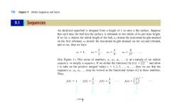
1106, , Chapter 13 Functions of Several Variables, , 23. f(x, y, z)  x 2eyz;, , P(2, 3, 0), v  i  2j  3k, , 24. f(x, y, z)  ln(x  y 2  z 2) ;, v  3i  2j  k, 2, , 25. f(x, y, z)  x 2y cos 2z;, , P(1, 2, 1),, , P 1 1, 2, p4 2 ,, , 26. f(x, y, z)  ex(2 cos y  3 sin z);, v  2i  j  3k, , S, , vijk, , P 1 1, p6 , p6 2 ,, , 400, 300, , y, 27. f(x, y, z)  x tan1 a b ;, z, , P(3, 2, 2),, , 28. f(x, y, z)  x 2 sin1 yz;, , 1, P(2, 1, 0), v , (i  j  k), 13, , v  i  2j  k, , In Exercises 29–32, find the directional derivative of the function, f at the point P in the direction from P to the point Q., , P, 200, , Note: This path is called the path of steepest ascent., , 43. Path of Steepest Descent The figure shows a topographical, map of a 620-ft hill with contours at 100-ft intervals., , 29. f(x, y)  x 3  y 3; P(1, 2), Q(2, 5), 30. f(x, y)  xey;, , P(2, 0),, , Q(1, 2), , 31. f(x, y, z)  x sin(2y  3z);, 32. f(x, y, z) , , xy, ;, yz, , 600, 500, , p, P 1 1, p4 , 12, 2,, , N, A, , Q 1 3, p2 , p4 2, , W, , E, S, , C, D, , P(2, 1, 1), Q(3, 2, 2), , 620 600 500 400, , 300, , 200, , B, , In Exercises 33–36, find a vector giving the direction in which, the function f increases most rapidly at the point P. What is the, maximum rate of increase?, 33. f(x, y)  22x  3y 2; P(3, 2), 34. f(x, y)  e2x cos y; P 1 0, p4 2, , 35. f(x, y, z)  x 3  2xz  2yz 2  z 3; P(1, 3, 2), 36. f(x, y, z)  ln(x 2  2y 2  3z 2) ; P(1, 2, 1), In Exercises 37–40, find a vector giving the direction in which, the function f decreases most rapidly at the point P. What is the, maximum rate of decrease?, 37. f(x, y)  tan1(2x  y); P(0, 0), 38. f(x, y)  xey ;, 2, , P(1, 0), , y, x, 39. f(x, y, z)   ;, y, z, , P(1, 1, 2), , 40. f(x, y, z)  1xy cos z;, , P 1 4, 1, p4 2, , 41. The height of a hill (in feet) is given by, h(x, y)  20(16  4x 2  3y 2  2xy  28x  18y), where x is the distance (in miles) east and y the distance (in, miles) north of Bolton. In what direction is the slope of the, hill steepest at the point 1 mile north and 1 mile east of, Bolton? What is the steepest slope at that point?, 42. Path of Steepest Ascent The following figure shows the contour map of a hill with its summit denoted by S. Draw the, curve from P to S that is associated with the path you will, take to reach the summit by ascending the direction of the, greatest increase in altitude., Hint: Study Figure 10., , a. If you start from A and proceed in a southwesterly direction, will you be ascending, descending, or neither, ascending nor descending? What if you start from B?, b. If you start from C and proceed in a westerly direction,, will you be ascending, descending, or neither ascending, nor descending?, c. If you start from D, in what direction should you proceed, to have the steepest ascent?, d. If you want to climb to the summit of the hill using the, gentlest ascent, would you start from the east or the west?, 44. Steady-State Temperature Consider the upper half-disk, H  {(x, y) 冟 x 2  y 2 1, y  0} (see the figure). If the, temperature at points on the upper boundary is kept at, 100°C and the temperature at points on the lower boundary, is kept at 50°C, then the steady-state temperature at any, point (x, y) inside the half-disk is given by, T(x, y)  100 , , 1  x 2  y2, 100, tan1, p, 2y, , y, , T  100, , 1 T  50, , 0, , 1, , x

Page 35 :
13.6, Find the rate of change of the temperature at the point, P 1 12, 12 2 in the direction of the vector v  2i  3j., , 45. Steady-State Temperature Consider the upper half-disk, H  {(x, y) 冟 x 2  y 2 1, y  0} (see the figure). If the, temperature at points on the upper boundary is kept at, 100°C and the temperature at points on the lower boundary, is kept at 0°C, then the steady-state temperature at any point, (x, y) inside the half-disk is given by, T(x, y) , , 2y, 200, tan1, p, 1  x 2  y2, , 1, a. Find the gradient of T at the point 1 17, 4 , 4 2 , and interpret, your result., b. Sketch the isothermal curve of T passing through the, 1, point 1 17, 4 , 4 2 and the gradient vector §T at that point on, the same coordinate system., , y, , Directional Derivatives and Gradient Vectors, , 50. Cobb-Douglas Production Function The output of a finished product is given by the production function, f(x, y)  100x 0.6y 0.4, where x stands for the number of units of labor and y stands, for the number of units of capital. Currently, the amount, being spent on labor is 500 units, and the amount being, spent on capital is 250 units. If the manufacturer wishes to, expand production by injecting an additional 10 units into, labor, how much more should be put into capital to maximize the increase in output?, 51. The figure shows the contour map of a function f of two, variables x and y. Use it to estimate the directional derivative of f at P0 in the indicated direction., y, 20, 4, , 25, 30, , P0, , 35, , 3, P1, , 2, , T  100, , 1107, , 40, , 1, 0, 1, , T0, , 0, , 1, , x, , 2, , 3, , 4, , 5, , 6, , 7, , 8, , 9, , x, , Hint: If u is a unit vector having indicated direction, then, , 46. The temperature at a point P(x, y, z) of a solid ball, of radius 4 with center at the origin is given by, T(x, y, z)  xy  yz  xz. Find the direction in which, T is increasing most rapidly at P(1, 1, 2)., 47. Let T(x, y, z) represent the temperature at a point P(x, y, z), of a region R in space. If the isotherms of T are concentric, spheres, show that the temperature gradient §T points either, toward or away from the center of the spheres., Hint: Recall that the isotherms of T are the sets on which T is constant., , 48. Suppose the temperature at the point (x, y) on a thin sheet of, metal is given by, T(x, y) , , 1, , 100(1  3x  2y), 1  2x 2  3y 2, , degrees Fahrenheit. In what direction will the temperature be, increasing most rapidly at the point (1, 2)? In what direction, will it be decreasing most rapidly?, 49. The temperature (in degrees Fahrenheit) at a point (x, y) on, a metal plate is, T(x, y)  90  6x 2  2y 2, An insect located at the point (1, 1) crawls in the direction, in which the temperature drops most rapidly., a. Find the path of the insect., b. Sketch a few level curves of T and the path found in, part (a)., , Du f(P0) ⬇, , f(P1)  f(P0), d(P0, P1), , when f(Pi) is the value of f at Pi (i  0, 1) and d(P0, P1) is the distance between P0 and P1., , 52. A rectangular metal plate of dimensions 8 in. 4 in. is, placed on a rectangular coordinate system with one corner at, the origin and the longer side along the positive x-axis. The, figure shows the contour map of the function f describing, the temperature of the plate in degrees Fahrenheit. Use the, contour map to estimate the rate of change of the temperature at the point (3, 1) in the direction from the point (3, 1), toward the point (5, 4)., y (in.), 4, , (5, 4), , 3, , 60, , 2, (3, 1), , 1, , 90 85, 0, , 1, , 2, , 3, , 4, , 65, , 75 70, , 80, 5, , 6, , 7, , 8 x (in.), , Hint: See Exercise 51., , 53. Suppose that f is differentiable, and suppose that the directional derivative of f at the origin attains a maximum value, of 5 in the direction of the vector from the origin to the, point (3, 4). Find §f(0, 0) .

Page 36 :
1108, , Chapter 13 Functions of Several Variables, , 54. Find unit vector(s) u  具u 1, u 2典 such that the directional, derivative of f(x, y)  x 2  exy at the point (1, 0) in the, direction of u has value 1., cas In Exercises 55 and 56, (a) Plot several level curves of each, , pair of functions f and t using the same viewing window, and, (b) Show analytically that each level curve of f intersects all, level curves of t at right angles., 55. f(x, y)  x 2  y 2,, , t(x, y)  xy, , 56. f(x, y)  ex cos y,, , t(x, y)  ex sin y, , 57. Let f(x, y)  x 2  y 2, and let t(x, y)  x 2  y 2. Find the, direction in which f increases most rapidly and the direction, in which t increases most rapidly at (0, 0). Is Theorem 3, applicable here?, , 13.7, , In Exercises 58–62, determine whether the statement is true or, false. If it is true, explain why it is true. If it is false, give an, example to show why it is false., 58. If f is differentiable at each point, then the directional derivative of f exists in all directions., 59. If f is differentiable at each point, then the value of the, directional derivative at any point in a given direction, depends only on the direction and the partial derivatives, fx and fy at that point., 60. If fx(a, b)  0 and fy(a, b)  0, then §f(a, b)  0., 61. The maximum value of Du f(x, y) is 2f 2x (x, y)  f 2y (x, y)., 62. If §f is known, then we can determine f completely., , Tangent Planes and Normal Lines, One compelling reason for studying the tangent line to a curve is that the curve may be, approximated by its tangent line near a point of tangency (Figure 1). Answers to questions about the curve near a point of tangency may be obtained indirectly by analyzing, the tangent line, a relatively simple task, rather than by studying the curve itself. As you, might recall, both the approximation of the change in a function using its differential, and Newton’s method for finding the zeros of a function are based on this observation., Our motivation for studying tangent planes to a surface in space is the same as that, for studying tangent lines to a curve: Near a point of tangency, a surface may be approximated by its tangent plane (Figure 1). We will show later that approximating the change, in z  f(x, y) using the differential is tantamount to approximating this change by the, change in z on the tangent plane., z, y, y  f (x), T, z  f (x, y), 0, , FIGURE 1, Near a point of tangency, the tangent, line approximates the curve, and the, tangent plane approximates the surface., , y, 0, (a) The tangent line to a curve, , x, , x, (b) The tangent plane to a surface, , Geometric Interpretation of the Gradient, We begin by looking at the geometric interpretation of the gradient of a function. This, vector will play a central role in our effort to find the tangent plane to a surface., Suppose that the temperature T at any point (x, y) in the plane is given by the function f ; that is, T  f(x, y). Then the level curve f(x, y)  c, where c is a constant, gives, the set of points in the plane that have temperature c (Figure 2). Recall that such a, curve is called an isothermal curve.

Page 37 :
13.7, y, , C, P, , (a, b), f (x, y)  c, , 0, , x, , FIGURE 2, The level curve C defined by, f(x, y)  c is an isothermal curve., , Tangent Planes and Normal Lines, , 1109, , If we are at the point P(a, b), in what direction should we move if we want to experience the greatest increase in temperature? Since the temperature remains constant if, we move along C, it seems reasonable to conjecture that proceeding in the direction, perpendicular to the tangent line to C at P will result in the greatest increase in temperature. But as we saw in Section 13.6, the function f (and hence the temperature), increases most rapidly in the direction given by its gradient §f(a, b). These observations suggest that the gradient §f(a, b) is perpendicular to the tangent line to the level, curve f(x, y)  c at P. That this is indeed the case can be demonstrated as follows:, Suppose that the curve C is represented by the vector function, r(t)  t(t)i  h(t)j, where t and h are differentiable functions, a  t(t 0) and b  h(t 0), and t 0 lies in the, parameter interval (Figure 3). Since the point (x, y)  (t(t), h(t)) lies on C, we have, f(t(t), h(t))  c, for all t in the parameter interval., y, ◊f (a, b), C, , P(a, b), r(t0), f (x, y)  c, , r(t), , FIGURE 3, The curve C may be represented by, r(t)  xi  yj  t(t)i  h(t)j., , t0, , t, , x, , 0, , Differentiating both sides of this equation with respect to t and using the Chain, Rule for a function of two variables, we obtain, f dx, f dy, , 0, x dt, y dt, Recalling that, §f(x, y) , , f, f, i, j, x, y, , and, , rⴕ(t) , , dy, dx, i, j, dt, dt, , we can write this last equation in the form, §f(x, y) ⴢ rⴕ(t)  0, In particular, when t  t 0, we have, §f(a, b) ⴢ rⴕ(t 0)  0, Thus, if rⴕ(t 0)  0, the vector §f(a, b) is orthogonal to the tangent vector rⴕ(t 0) at, P(a, b). Loosely speaking, we have demonstrated the following:, §f is orthogonal to the level curve f(x, y)  c at P., , See Figure 3., , EXAMPLE 1 Let f(x, y)  x 2  y 2. Find the level curve of f passing through the point, (5, 3) . Also, find the gradient of f at that point, and make a sketch of both the level, curve and the gradient vector.

Page 38 :
1110, , Chapter 13 Functions of Several Variables, y, , 4, 4 0, 4, , Solution Since f(5, 3)  25  9  16, the required level curve is the hyperbola, x 2  y 2  16. The gradient of f at any point (x, y) is, , Tangent, line, , §f(x, y)  2xi  2y j, , (5, 3), x, , 4, , and, in particular, the gradient of f at (5, 3) is, §f(5, 3)  10i  6j, , ◊ f (5, 3), , The level curve and §f(5, 3) are shown in Figure 4., FIGURE 4, The gradient §f(5, 3) is orthogonal to, the level curve x 2  y 2  16 at (5, 3)., , EXAMPLE 2 Refer to Example 1. Find equations of the normal line and the tangent, line to the curve x 2  y 2  16 at the point (5, 3)., Solution We think of the curve x 2  y 2  16 as the level curve f(x, y)  k of the, function f(x, y)  x 2  y 2 for k  16. From Example 1 we see that §f(5, 3) , 10i  6j. Since this gradient is normal to the curve x 2  y 2  16 at (5, 3) (see Figure 4), we see that the slope of the required normal line is, m1  , , 6, 3, , 10, 5, , Therefore, an equation of the normal line is, 3, y  3   (x  5), 5, , 3, y x6, 5, , or, , The slope of the required tangent line is, m2  , , 1, 5, , m1, 3, , so an equation of the tangent line is, y3, , 5, (x  5), 3, , or, , y, , 5, 16, x, 3, 3, , Next, suppose that F(x, y, z)  k is the level surface S of a differentiable function, F defined by T  F(x, y, z). You may think of the function F as giving the temperature at any point (x, y, z) in space and interpret the following argument in terms of this, application., Suppose that P(a, b, c) is a point on S and let C be a smooth curve on S passing, through P. Then C can be described by the vector function, r(t)  f(t)i  t(t)j  h(t)k, where f(t 0)  a, t(t 0)  b, h(t 0)  c, and t 0 is a point in the parameter interval (Figure 5)., z, F(a, b, c), r'(t0), , S, , P(a, b, c), C, , FIGURE 5, The curve C is described by, r(t)  f(t)i  t(t)j  h(t)k with, P(a, b, c) corresponding to t 0., , t0, , 0, , t, , y, x

Page 39 :
13.7, , Tangent Planes and Normal Lines, , 1111, , Since the point (x, y, z)  ( f(t), t(t), h(t)) lies on S, we have, F( f(t), t(t), h(t))  k, for all t in the parameter interval. If r is differentiable, then we can use the Chain Rule, to differentiate both sides of this equation to obtain, F dx, F dy, F dz, , , 0, x dt, y dt, z dt, z, , This is the same as, [Fx(x, y, z)i  Fy(x, y, z)j  Fz(x, y, z)k] ⴢ c, , F(a, b, c), , dy, dx, dz, i, j, kd  0, dt, dt, dt, , r'(t), , or, in an even more abbreviated form,, , P, , §F(x, y, z) ⴢ rⴕ(t)  0, , C, , In particular, at t  t 0 we have, , 0, , §F(a, b, c) ⴢ rⴕ(t 0)  0, y, , x, , FIGURE 6, The gradient §F(a, b, c) is orthogonal, to the tangent vector of every curve, on S passing through P(a, b, c)., , This shows that if rⴕ(t 0)  0, then the gradient vector §F(a, b, c) is orthogonal to, the tangent vector rⴕ(t 0) to C at P (Figure 6). Since this argument holds for any differentiable curve passing through P(a, b, c) on S, we have shown that §F(a, b, c) is, orthogonal to the tangent vector of every curve on S passing through P. Thus, loosely, speaking, we have demonstrated the following result., , §F is orthogonal to the level surface F(x, y, z)  0 at P., , Note Interpreting the function F as giving the temperature at any point (x, y, z) in, space as was suggested earlier, we see that the level surface F(x, y, z)  k gives all, points (x, y, z) in space whose temperature is k. The result that was just derived simply states that if you are at any point on this surface, then moving away from it in a, direction of §F (perpendicular to the surface at that point) will result in the greatest, increase in temperature., z, , F(0, 3, 4), , 5, , EXAMPLE 3 Let F(x, y, z)  x 2  y 2  z 2. Find the level surface that contains the, point (0, 3, 4). Also, find the gradient of F at that point, and make a sketch of both the, level surface and the gradient vector., , 5, , y, , 5, x, , FIGURE 7, The gradient §F(0, 3, 4) is orthogonal, to the level surface x 2  y 2  z 2  25, at (0, 3, 4)., , Solution Since F(0, 3, 4)  0  9  16  25, the required level surface is the sphere, x 2  y 2  z 2  25 with center at the origin and radius 5. The gradient of F at any, point (x, y, z) is, §F(x, y, z)  2xi  2yj  2zk, so the gradient of F at (0, 3, 4) is, §F(0, 3, 4)  6j  8k, The level surface and §F(0, 3, 4) are sketched in Figure 7.

Page 40 :
1112, , Chapter 13 Functions of Several Variables, , Tangent Planes and Normal Lines, We are now in a position to define a tangent plane to a surface in space. But before, doing so, let’s digress a little to talk about the representation of surfaces in space. Up, to now, we have assumed that a surface in space is described by a function f with, explicit representation z  f(x, y)., Another way of describing a surface in space is via a function that is represented, implicitly by the equation, F(x, y, z)  0, , (1), , Here, F is a function of the three variables x, y, and z described by the equation, w  F(x, y, z). Thus, we can think of Equation (1) as representing a level surface, of F., For a surface S that is given explicitly by z  f(x, y), we define, F(x, y, z)  z  f(x, y), This shows that we can also view S as the level surface of F given by Equation (1)., For example, the surface described by z  x 2  2y 2  1 can be viewed as the level, surface of F defined by F(x, y, z)  0, where F(x, y, z)  z  x 2  2y 2  1., To define a tangent plane, let S be a surface described by F(x, y, z)  0, and let, P(a, b, c) be a point on S. Then, as we saw earlier, the gradient §F(a, b, c) at P is, orthogonal to the tangent vector of every curve on S passing through P (Figure 8). This, suggests that we define the tangent plane to S at P to be the plane passing through P, and containing all these tangent vectors. Equivalently, the tangent plane should have, §F(a, b, c) as a normal vector., z, F(a, b, c), S, P, F(x, y, z), , FIGURE 8, The tangent plane to S at P contains, the tangent vectors to all curves, on S passing through P., , t0, , t, , 0, y, x, , DEFINITIONS Tangent Plane and Normal Line, Let P(a, b, c) be a point on the surface S described by F(x, y, z)  0, where F, is differentiable at P, and suppose that §F(a, b, c)  0. Then the tangent plane, to S at P is the plane that passes through P and has normal vector §F(a, b, c)., The normal line to S at P is the line that passes through P and has the same, direction as §F(a, b, c)., , Using Equation (4) from Section 11.5, we see that an equation of the tangent plane, is, Fx(a, b, c)(x  a)  Fy(a, b, c)(y  b)  Fz (a, b, c)(z  c)  0, , (2)

Page 41 :
13.7, , Tangent Planes and Normal Lines, , 1113, , and using Equation (2) of Section 11.5, we see that the equations of the normal line, (in symmetric form) are, yb, xa, zc, , , Fx(a, b, c), Fy(a, b, c), Fz(a, b, c), , (3), , EXAMPLE 4 Find equations of the tangent plane and normal line to the ellipsoid with, equation 4x 2  y 2  4z 2  16 at the point (1, 2, 12)., Solution The given equation can be written in the form F(x, y, z)  0, where, F(x, y, z)  4x 2  y 2  4z 2  16. The partial derivatives of F are, Fx(x, y, z)  8x,, , z, , Fy(x, y, z)  2y,, , and, , Fz(x, y, z)  8z, , In particular, at the point (1, 2, 12), , L, , Fx(1, 2, 12)  8,, T, , Fy(1, 2, 12)  4,, , and, , Fz(1, 2, 12)  812, , Then, using Equation (2), we find that an equation of the tangent plane to the ellipsoid, at (1, 2, 12) is, 8(x  1)  4(y  2)  812(z  12)  0, y, , x, , FIGURE 9, The tangent plane and normal line to, the ellipsoid 4x 2  y 2  4z 2  16, at (1, 2, 12)., , or 2x  y  212z  8. Next, using Equation (3), we obtain the following parametric equations of the normal line:, y2, x1, z  12, , , 8, 4, 812, , or, , x1, z  12, y2, 2, 212, , The tangent plane and normal line are shown in Figure 9., , EXAMPLE 5 Find equations of the tangent plane and normal line to the graph of the, function f defined by f(x, y)  4x 2  y 2  2 at the point where x  1 and y  1., Solution, , Here, the surface is defined by, z  f(x, y)  4x 2  y 2  2, , z, , and we recognize it to be a paraboloid. This equation can be rewritten in the form, 12, , F(x, y, z)  z  f(x, y)  0, where F(x, y, z)  z  4x  y 2  2. The partial derivatives of F are, , 1100, , 2, , Fx(x, y, z)  8x,, 7 (1, 1, 7), , Fy(x, y, z)  2y,, , and, , Fz(x, y, z)  1, , If x  1 and y  1, then z  f(1, 1)  4  1  2  7. At the point (1, 1, 7) we have, Fx(1, 1, 7)  8,, , T, , Fy(1, 1, 7)  2,, , and, , Fz(1, 1, 7)  1, , Then, using Equation (2), we find an equation of the tangent plane to the paraboloid, at (1, 1, 7) to be, , L, , 8(x  1)  2(y  1)  1(z  7)  0, 1, , 1 2, 3, , y, , x, , FIGURE 10, The tangent plane and normal line to, the paraboloid z  4x 2  y 2  2 at, (1, 1, 7)., , or 8x  2y  z  3. Next, using Equation (3), we find that the parametric equations, of the normal line at (1, 1, 7) are, y1, x1, z7, , , 8, 2, 1, The tangent plane and normal line are shown in Figure 10., , Copyright 2009 Cengage Learning. All Rights Reserved. May not be copied, scanned, or duplicated, in whole or in part.

Page 42 :
1114, , Chapter 13 Functions of Several Variables, , Using the Tangent Plane of f to Approximate, the Surface z ⴝ f(x, y), We conclude this section by showing that in approximating the change ⌬z in, z  f(x, y) as (x, y) changes from (a, b) to (a  ⌬x, b  ⌬y) by the differential, dz  fx(a, b) ⌬x  fy(a, b) ⌬y, we are in effect using the tangent plane of f near P(a, b), to approximate the surface z  f(x, y) near P(a, b)., We begin by finding an expression for the tangent plane to the surface z  f(x, y), at (a, b). Writing z  f(x, y) in the form F(x, y, z)  z  f(x, y)  0 we see that, Fx(a, b, c)  fx(a, b),, , Fy(a, b, c)  fy(a, b),, , Fz(a, b, c)  1, , and, , Using Equation (2), we find that the required equation is, fx(a, b)(x  a)  fy(a, b)(y  b)  (z  c)  0, or, z  f(a, b)  fx(a, b) ⌬x  fy(a, b) ⌬y, , c  f(a, b), , (4), , But the expression on the right is just the differential of f at (a, b). So Equation (4), implies that dz  z  f(a, b); that is, dz represents the change in height of the tangent, plane (Figure 11)., z, (a  Δ x, b  Δy, f(a  Δ x, b  Δy)), z  f (x, y), , dz, , Δz, , (a, b, f (a, b)), Tangent plane, 0, (a  Δ x, b), y, , FIGURE 11, The relationship between ⌬z and dz, , x, , (a  Δ x, b  Δy), , (a, b), , By Theorem 1 of Section 13.4 we have, ⌬z  fx(a, b) ⌬x  fy(a, b) ⌬y  e1 ⌬x  e2 ⌬y, or, ⌬z  dz  e1 ⌬x  e2 ⌬y, where e1 and e2 are functions of ⌬x and ⌬y that approach 0 as ⌬x and ⌬y approach 0., Therefore, as was pointed out in Section 13.4, ⌬z ⬇ dz if ⌬x and ⌬y are small. Recalling the meaning of ⌬z (see Figure 11), we see that we are using the tangent plane at, (a, b) to approximate the surface z  f(x, y) when (x, y) is close to (a, b)., , 13.7, , CONCEPT QUESTIONS, , 1. a. Consider the level curve f(x, y)  c, where f is differentiable and c is a constant. What can you say about §f at, a point P on the level curve? Illustrate with a figure., b. Repeat part (a) for a level surface F(x, y, z)  c., , 2. a. Define the tangent plane to a surface S described by, F(x, y, z)  0 at the point P(a, b, c) on S. Illustrate with, a figure and give an equation of the tangent plane., b. Repeat part (a) for the normal line to S at P.

Page 43 :
13.7, , 13.7, , 1. f(x, y)  y 2  x 2; P(1, 2), , 2. f(x, y)  4x 2  y 2; P 1 13, 2 , 12, 3. f(x, y)  x 2  y;, , P(1, 3), , y, 29. z  tan1 a b ;, x, , Pa1, 1,, , p, b, 4, , 30. z  x cos y  0;, , Pa2,, , p, , 1b, 3, , 31. sin xy  3z  3;, , P(0, 3, 1), , 32. e (cos y  1)  2z  2;, x, , 4. f(x, y)  2x  3y; P(3, 4), , x2, a, , 1 313, 2 , 22, , y2, x2, ,  1;, 9, 16, , 6. x 4  x 2  y 2  0;, 4, , 1 12, 134 2, , xx 0, , 2, , 8. 2x  y  exy  2;, , 2, , In Exercises 9–14, sketch (a) the level surface of the function F, that passes through the point P and (b) the gradient of F at P., 9. F(x, y, z)  x 2  y 2  z 2;, , 2, , a2, , P(2, 3, 1), 2, , P 1 2, 12, 0 2, , 15. x 2  4y 2  9z 2  17;, , P(2, 1, 1), , 16. 2x 2  y 2  3z 2  2;, , P(2, 3, 1), , 17. x  2y  4z  4;, , P(4, 2, 1), , 2, , 2, , 2, , 19. xy  yz  xz  11;, 20. xyz  4;, , 22. z  y  2x ;, 2, , 2, , 25. z  xey;, , a, , P(2, 0, 2), , 26. z  e sin py;, 27. z  ln(xy  1);, x, 28. z  ln ;, y, , P(0, 1, 0), P(3, 0, 0), , P(2, 2, 0), , 1, , , , yy0, b2, , , , zz 0, c2, , 1, , , , yy0, b2, , , , zz 0, c2, , 1, , 2, , , , 2yy0, b2, ,  c(z  z 0), , 37. Find the points on the sphere x 2  y 2  z 2  14 at which, the tangent plane is parallel to the plane x  2y  3z  12., , P(2, 4, 8), , 3, , x, , c2, , at the point (x 0, y0, z 0) can be written as, 2xx 0, , P(1, 2, 25), , 24. x  xy  z  2x  6  0;, 2, , P(1, 0, 2), , P(1, 2, 3), , 23. xz 2  yx 2  y 2  2x  3y  6  0;, 3, , z2, , at the point (x 0, y0, z 0) , and express it in a form similar to, that of Exercise 34., , P(2, 1, 2), , 21. z  9x 2  4y 2;, , , , 36. Show that an equation of the tangent plane to the elliptic, paraboloid, y2, x2,  2  cz, 2, a, b, , 18. x  y  z  2xy  4xz  x  y  12;, 2, , b, , 2, , 35. Find an equation of the tangent plane to the hyperboloid of, two sheets, y2, x2, z2,  2 21, 2, a, b, c, , P(1, 3, 2), , In Exercises 15–32, find equations for the tangent plane and, the normal line to the surface with the equation at the given, point., , 2, , 2, , xx 0, , P(0, 2, 4), , 13. F(x, y, z)  x  y  z ;, , 2, , y2, , at the point (x 0, y0, z 0) can be written as, , P(1, 1, 2), , 12. F(x, y, z)  2x  3y  z;, 14. F(x, y, z)  xy;, , , , 34. Show that an equation of the tangent plane to the hyperboloid, y2, x2, z2, , , 1, a2, b2, c2, , P(1, 2, 2), , 10. F(x, y, z)  z  x 2  y 2;, , 2, , a, , ( 15, 1), , (1, 1), , 11. F(x, y, z)  x 2  y 2;, , 2, , at the point (x 0, y0, z 0) can be written as, , 7. x  2x y  y  9x  9y  0;, 2 2, , P(0, 0, 2), , 33. Show that an equation of the tangent plane to the ellipsoid, , In Exercises 5–8, find equations of the normal and tangent lines, to the curve at the given point., , 4, , 1115, , EXERCISES, , In Exercises 1–4, sketch (a) the level curve of the function f that, passes through the point P and (b) the gradient of f at P., , 5., , Tangent Planes and Normal Lines, , P(2, 1, 3), , P(1, 2, 1), , 38. Find the points on the hyperboloid of two sheets, x 2  2y 2  z 2  4 at which the tangent plane is parallel, to the plane 2x  2y  4z  1., 39. Find the points on the hyperboloid of one sheet, 2x 2  y 2  z 2  1 at which the normal line is parallel to, the line passing through the points (1, 1, 2) and (3, 3, 3)., 40. Find the points on the surface x 2  4y 2  3z 2  2xy  16, at which the tangent plane is horizontal., , V Videos for selected exercises are available online at www.academic.cengage.com/login.

Page 44 :
1116, , Chapter 13 Functions of Several Variables, , 41. Two surfaces are tangent to each other at a point P if and, only if they have a common tangent plane at that point., Show that the elliptic paraboloid 2x 2  y 2  z  5  0, and the sphere x 2  y 2  z 2  6x  8y  z  17  0 are, tangent to each other at the point (1, 2, 1)., 42. Two surfaces are orthogonal to each other at a point of, intersection P if and only if their normal lines at P are, orthogonal. Show that the sphere x 2  y 2  z 2  17  0, and the elliptic paraboloid 2x 2  y  2z 2  2  0 are, orthogonal to each other at the point (1, 4, 0)., , parametric equations of the tangent line to C at the point, 1 122, 122, 1 2 ., In Exercises 46–49, determine whether the statement is true or, false. If it is true, explain why it is true. If it is false, give an, example to show why it is false., 46. The tangent line at a point P on the level curve f(x, y)  c, is orthogonal to §f at P., 47. The line with equations, y1, x2, z, , , 4, 6, 2, , 43. Show that any line that is tangent to the ellipse, (x 2>a 2)  (y 2>b 2)  1 has the equation, , is perpendicular to the plane with equation 2x  3y  z  4., , (b cos u)x  (a sin u)y  ab, where u lies in the interval [0, 2p)., 44. Suppose that two surfaces F(x, y, z)  0 and G(x, y, z)  0, intersect along a curve C and that P(x 0, y0, z 0) is a point on, C. Show that the vector §F(x 0, y0, z 0), §G(x 0, y0, z 0) is, parallel to the tangent line to C at P. Illustrate with a sketch., 45. Refer to Exercise 44. Let C be the intersection of the sphere, x 2  y 2  z 2  2 and the paraboloid z  x 2  y 2. Find the, , 48. If an equation of the tangent plane at the point P0(x 0, y0, z 0), on the surface described by F(x, y, z)  0 is, ax  by  cz  d, then §F(x 0, y0, z 0)  k具a, b, c典 for some, scalar k., 49. The vector equation of the normal line passing through the, point P0 (x 0, y0, z 0) on the surface with equation, F(x, y, z)  0 is r(t)  具x 0, y0, z 0典  t §F(x 0, y0, z 0) ., , 13.8 Extrema of Functions of Two Variables, Relative and Absolute Extrema, In Chapter 3 we saw that the solution of a problem often reduces to finding the extreme, values of a function of one variable. A similar situation arises when we solve problems, involving a function of two or more variables., For example, suppose that the Scandi Company manufactures computer desks in, both assembled and unassembled versions. Then its weekly profit P is a function of, the number of assembled units, x, and the number of unassembled units, y, sold per, week; that is, P  f(x, y). A question of paramount importance to the manufacturer is:, How many assembled desks and how many unassembled desks should the company, manufacture per week to maximize its weekly profit? Mathematically, the problem is, solved by finding the values of x and y that will make f(x, y) a maximum., In this section and the next section we will focus our attention on finding the extrema, of a function of two variables. As in the case of a function of one variable, we distinguish between the relative (or local) extrema and the absolute extrema of a function of, two variables., , DEFINITION Relative Extrema of a Function of Two Variables, Let f be a function defined on a region R containing the point (a, b). Then f has, a relative maximum at (a, b) if f(x, y) f(a, b) for all points (x, y) in an open, disk containing (a, b). The number f(a, b) is called a relative maximum value., Similarly, f has a relative minimum at (a, b) with relative minimum value, f(a, b) if f(x, y)  f(a, b) for all points (x, y) in an open disk containing (a, b).

Page 45 :
13.8, , Extrema of Functions of Two Variables, , 1117, , Loosely speaking, f has a relative maximum at (a, b) if the point (a, b, f(a, b)) is, the highest point on the graph of f when compared to all nearby points. A similar interpretation holds for a relative minimum., If the inequalities in this last definition hold for all points (x, y) in the domain of, f, then f has an absolute maximum (absolute minimum) at (a, b) with absolute maximum value (absolute minimum value) f(a, b). Figure 1 shows the graph of a function defined on a domain D with relative maxima at (a, b) and (e, t) and a relative minimum at (c, d). The absolute maximum of f occurs at (e, t), and the absolute minimum, of f occurs at (h, i)., z, , Relative, maximum, , Absolute maximum, (also a relative, maximum), , Absolute, minimum, Relative, minimum (a, b), , FIGURE 1, The relative and absolute extrema of, the function f over the domain D, , x, , (h, i), , y, , (c, d) (e, t), , D, , Critical Points—Candidates for Relative Extrema, Figure 2a shows the graph of a function f with a relative maximum at a point (a, b), lying inside the domain of f. As you can see, the tangent plane to the surface z  f(x, y), at the point (a, b, f(a, b)) is horizontal. This means that all the directional derivatives, of f at (a, b), if they exist, must be zero. In particular, fx(a, b)  0 and fy(a, b)  0., Next, Figure 2b shows the graph of a function with a relative maximum at a point, (a, b) . Note that both fx(a, b) and fy(a, b) do not exist because the surface z  f(x, y), has a point (a, b, f(a, b)) that looks like a jagged mountain peak., z, (a, b, f (a, b)), fy(a, b)  0, fx(a, b)  0, , z, (a, b, f (a, b)), , FIGURE 2, At a relative extremum of f, either, fx  fy  0 or one or both partial, derivatives do not exist., , 0, , 0, x, , (a, b), , (a) fx  fy  0, , y, , x, , (a, b), , y, , (b) fx and fy do not exist., , You are encouraged to draw similar graphs of functions having relative minima at, points lying inside the domain of the functions. All of these points are critical points, of a function of two variables., , Copyright 2009 Cengage Learning. All Rights Reserved. May not be copied, scanned, or duplicated, in whole or in part.

Page 46 :
1118, , Chapter 13 Functions of Several Variables, , DEFINITION Critical Points of a Function, Let f be defined on an open region R containing the point (a, b). We call (a, b), a critical point of f if, a. fx and/or fy do not exist at (a, b) or, b. both fx(a, b)  0 and fy(a, b)  0., , The next theorem tells us that the relative extremum of a function f defined on an, open region can occur only at a critical point of f., , THEOREM 1 The Critical Points of f Are Candidates for Relative Extrema, If f has a relative extremum (relative maximum or relative minimum) at a point, (a, b) in the domain of f, then (a, b) must be a critical point of f., , PROOF If either fx or fy does not exist at (a, b), then (a, b) is a critical point of f., , So suppose that both fx(a, b) and fy(a, b) exist. Let t(x)  f(x, b). If f has a relative, extremum at (a, b), then t has a relative extremum at a, so by Theorem 1 of Section 3.1,, t¿(a)  0. But, f(a  h, b)  f(a, b),  fx(a, b), h→0, h, , t¿(a)  lim, , Therefore, fx(a, b)  0. Similarly, by considering the function f(y)  f(a, y), we obtain, fy(a, b)  0. Thus, (a, b) is a critical point of f., , EXAMPLE 1 Let f(x, y)  x 2  y 2  4x  6y  17. Find the critical point of f, and, , z, , show that f has a relative minimum at that point., z  f (x, y), , 3, , 1, , x, , 0, , 1, , 2, (2, 3), , and, , fy(x, y)  2y  6  2(y  3), , Observe that both fx and fy are continuous for all values of x and y. Setting fx and fy, equal to zero, we find that x  2 and y  3, so (2, 3) is the only critical point of f., Next, to show that f has a relative minimum at this point, we complete the squares in, x and y and write f(x, y) in the form, , (2, 3, 4), , 2, , 1, , To find the critical point of f, we compute, , fx(x, y)  2x  4  2(x  2), , 4, , 2, , Solution, , f(x, y)  (x  2)2  (y  3)2  4, , 3, y, , FIGURE 3, The function f has a relative minimum, at (2, 3)., , Notice that (x  2)2  0 and (y  3)2  0, so f(x, y)  4 for all (x, y) in the domain, of f. Therefore, f(2, 3)  4 is a relative minimum value of f. In fact, we have shown, that 4 is the absolute minimum value of f. The graph of f shown in Figure 3 confirms, this result., , EXAMPLE 2 Let f(x, y)  3  2x 2  y 2. Show that (0, 0) is the only critical point, , of f and that f(0, 0)  3 is a relative maximum value of f., Solution, , The partial derivatives of f are, fx(x, y)  , , x, 2x  y, 2, , 2, , and, , fy(x, y)  , , y, 2x  y 2, 2

Page 47 :
13.8, z, , 3 (0, 0, 3), z3, , x2  y2, , (0, 0), 3, , 3, , y, , x, , FIGURE 4, The function f has a relative maximum, at (0, 0)., , Extrema of Functions of Two Variables, , 1119, , Since both fx(x, y) and fy(x, y) are undefined at (0, 0), we conclude that (0, 0) is a critical point of f. Also, fx(x, y) and fy(x, y) are not both equal to zero at any point. This, tells us that (0, 0) is the only critical point of f. Finally, since 2x 2  y 2  0 for all, values of x and y, we see that f(x, y) 3 for all points (x, y). We conclude that, f(0, 0)  3 is a relative (indeed, the absolute) maximum of f. The graph of f shown in, Figure 4 confirms this result., As in the case of a function of one variable, a critical point of a function of two, variables is only a candidate for a relative extremum of the function. A critical point, need not give rise to a relative extremum, as the following example shows., , EXAMPLE 3 Show that the point (0, 0) is a critical point of f(x, y)  y 2  x 2 but, that it does not give rise to a relative extremum of f., Solution, , The partial derivatives of f,, fx(x, y)  2x, , and, , fy(x, y)  2y, , are continuous everywhere. Since fx and fy are both equal to zero at (0, 0), we conclude, that (0, 0) is a critical point of f and that it is the only candidate for a relative extremum, of f. But notice that for points on the x-axis we have y  0, so f(x, y)  x 2  0 if, x  0; and for points on the y-axis we have x  0, so f(x, y)  y 2  0 if y  0. Therefore, every open disk containing (0, 0) has points where f takes on positive values as, well as points where f takes on negative values. This shows that f(0, 0)  0 cannot be, a relative extremum of f. The graph of f is shown in Figure 5. The point (0, 0, 0) is, called a saddle point., , z, , FIGURE 5, The point (0, 0) is a critical point, of f(x, y)  y 2  x 2, but it does not, give rise to a relative extremum of f., , y, x, , fx (0, 0)  0, , fy(0, 0)  0, , As we have observed, the critical point (0, 0) in Example 3 does not yield a relative, maximum or minimum. In general, a critical point of a differentiable function of two, variables that does not give rise to a relative extremum is called a saddle point. A saddle point is the analog of an inflection point for the case of a function of one variable., , The Second Derivative Test for Relative Extrema, In Examples 1 and 3 we were able to determine, either by inspection or with the help, of simple algebraic manipulations, whether f did or did not possess a relative extremum, at a critical point. For more complicated functions, the following test may be used., This test is the analog of the Second Derivative Test for a function of one variable. Its, proof will be omitted.

Page 48 :
1120, , Chapter 13 Functions of Several Variables, , THEOREM 2 The Second Derivative Test for a Function of Two Variables, Suppose that f has continuous second-order partial derivatives on an open region, containing a critical point (a, b) of f. Let, D(x, y)  fxx(x, y)fyy(x, y)  f 2xy(x, y), a. If D(a, b), value., b. If D(a, b), c. If D(a, b), d. If D(a, b), ,  0 and fxx(a, b)  0, then f(a, b) is a relative maximum,  0 and fxx(a, b)  0, then f(a, b) is a relative minimum value.,  0, then (a, b, f(a, b)) is a saddle point.,  0, then the test is inconclusive., , EXAMPLE 4 Find the relative extrema of f(x, y)  x 3  y 2  2xy  7x  8y  2., Solution, , First, we find the critical points of f. Since, fx(x, y)  3x 2  2y  7, , and, , fy(x, y)  2y  2x  8, , are both continuous for all values of x and y, the only critical points of f, if any, are, found by solving the system of equations fx(x, y)  0 and fy(x, y)  0, that is, by, solving, 3x 2  2y  7  0, , and, , 2y  2x  8  0, , From the second equation we obtain y  x  4, which upon substitution into the first, equation yields, 3x 2  2x  1  0, , or, , (3x  1)(x  1)  0, , 13 or, 11, 3 and, , Therefore, x , x  1. Substituting each of these values of x into the expression, for y gives y , y  5, respectively. Therefore, the critical points of f are 1 13, 113 2, and (1, 5)., Next, we use the Second Derivative Test to determine the nature of each of these, critical points. We begin by computing fxx(x, y)  6x, fyy(x, y)  2, fxy(x, y)  2, and, D(x, y)  fxx(x, y)fyy(x, y)  f 2xy(x, y),  (6x)(2)  (2)2  4(3x  1), , To test the point 1 13, 113 2 , we compute, , D 1 13, 113 2  4(1  1)  8  0, , from which we deduce that 1 13, 113 2 gives rise to the saddle point 1 13, 113, 373, 27 2 of f., Next, to test the critical point (1, 5), we compute, D(1, 5)  4(3  1)  8  0, which indicates that (1, 5) gives a relative extremum of f. Since, fxx(1, 5)  6(1)  6  0, we see that (1, 5) yields a relative minimum of f. Its value is, f(1, 5)  (1)3  (5)2  2(1)(5)  7(1)  8(5)  2,  15, The graph and contour map of f are shown in Figures 6a and 6b.

Page 49 :
13.8, 2, , 4, , Extrema of Functions of Two Variables, , 1121, , y, , 6, 7, , 6, , 0, Saddle, point, , 15, , 5, , 14.3, , 10, 4, , 1, , Relative, minimum, , 2, , 12.7, , 3, , 0, 1, , 2, 2, , 2, , FIGURE 6, , 13.4, , (a) The graph of f (x, y)  x 3  y2  2xy  7x  8y  2, , 1, , 0, , 1, , 2, , x, , (b) The contour plot of f, , EXAMPLE 5 Priority Mail Regulations Postal regulations specify that the combined, length and girth of a package sent by priority mail may not exceed 108 in. Find the, dimensions of a rectangular package with the greatest possible volume satisfying these, regulations., Solution Let the length, width, and height of the package be x, y, and z inches respectively, as shown in Figure 7. Then the volume of the package is V  xyz. Observe that, the combined length and girth of the package is (x  2y  2z) inches. Clearly, we, should let this quantity be as large as possible, that is, we should let, , z, , x  2y  2z  108, , x, y, , FIGURE 7, The combined length and girth of, the package is x  2y  2z inches., , With the help of this equation we can express V as a function of two variables. For, example, solving the equation for x in terms of y and z, we obtain, x  108  2y  2z, which, upon substitution into the expression for V, gives, V  f(y, z)  (108  2y  2z)yz  108yz  2y 2z  2yz 2, To find the critical points of f, we set, fy  108z  4yz  2z 2  2z(54  2y  z)  0, and, fz  108y  2y 2  4yz  2y(54  y  2z)  0, Since y and z are both nonzero (otherwise, V would be zero), we are led to the system, 54  2y  z  0, 54  y  2z  0, Multiplying the second equation by 2 gives 108  2y  4z  0. Then subtracting this, equation from the first equation gives 54  3z  0, or z  18. Substituting this value, of z into either equation in the system then yields y  18. Therefore, the only critical, point of f is (18, 18) .

Page 50 :
1122, , Chapter 13 Functions of Several Variables, , We could use the Second Derivative Test to show that the point (18, 18) gives, a relative maximum of V, or, as in this situation, we can simply argue from physical, considerations that V must attain an absolute maximum at (18, 18). Finally, from the, equation, x  108  2y  2z, found earlier, we see that when y  z  18,, x  108  2(18)  2(18)  36, Therefore, the dimensions of the required package are 18 in., , 18 in., , 36 in., , Finding the Absolute Extremum Values, of a Continuous Function on a Closed Set, Recall that if f is a continuous function of one variable on a closed interval [a, b], then, the Extreme Value Theorem guarantees that f has an absolute maximum value and an, absolute minimum value. The analog of this theorem for a function of two variables, follows., , THEOREM 3 The Extreme Value Theorem for Functions of Two Variables, If f is continuous on a closed, bounded set D in the plane, then f attains an, absolute maximum value f(a, b) at some point (a, b) in D and an absolute minimum value f(c, d) at some point (c, d) in D., , The following procedure for finding the extreme values of a function of two variables is the analog of the one for finding the extreme values of a function of one variable discussed in Section 3.1., Finding the Absolute Extremum Values of f on a Closed, Bounded Set D, 1. Find the values of f at the critical points of f in D., 2. Find the extreme values of f on the boundary of D., 3. The absolute maximum value of f and the absolute minimum value of f are, precisely the largest and the smallest numbers found in Steps 1 and 2., , The justification for this procedure is similar to that for a function of one variable, on a closed interval [a, b]: If an absolute extremum of f occurs in the interior of D,, then it must also be a relative extremum of f, and hence it must occur at a critical point, of f. Otherwise, the absolute extremum of f must occur at a boundary point of D., , EXAMPLE 6 Find the absolute maximum and the absolute minimum values of the, function f(x, y)  2x 2  y 2  4x  2y  3 on the rectangle, D  {(x, y) 冟 0, , x, , 3, 0, , y, , 2}, , Solution Since f is a polynomial, it is continuous on the closed, bounded set D. Therefore, Theorem 3 guarantees the existence of an absolute maximum and an absolute, minimum value of f on D.

Page 51 :
13.8, Step 1, , y, , L3, , 2, L4, , Step 2, L2, , 1, , 0, , 1, , L1, , 2, , 1123, , To find the critical point of f in D, we set fx  4x  4  0 and, fy  2y  2  0. Solving this system of equations gives (1, 1) as, the only critical point of f. The value of f at this point is f(1, 1)  0., Next, we look for extreme values of f on the boundary of D. We can think, of this boundary as being made up of four line segments L 1, L 2, L 3, and L 4,, as shown in Figure 8., On L 1: Here y  0, so we have, f(x, 0)  2x 2  4x  3, , x, , 3, , Extrema of Functions of Two Variables, , 0, , x, , 3, , To find the extreme values of the continuous function f(x, 0) of one variable on, the closed bounded interval [0, 3], we use the method of Section 3.1. Setting, , FIGURE 8, The boundary of D consists of the four, line segments L 1, L 2, L 3, and L 4., , f ¿(x, 0)  4x  4  0, gives x  1 as the only critical number of f(x, 0) in (0, 3). Evaluating f(x, 0), at x  1, as well as at the endpoints of the interval [0, 3], gives f(0, 0)  3,, f(1, 0)  1, and f(3, 0)  9. Thus, f has the absolute minimum value of 1, and the absolute maximum value of 9 on L 1., On L 2: Here x  3, so we have, f(3, y)  y 2  2y  9, , 0, , y, , 2, , Setting f ¿(3, y)  2y  2  0 yields y  1 as the only critical number of, f(3, y) in (0, 2). Evaluating f(3, y) at the endpoints of [0, 2] and at the critical number y  1 gives f(3, 0)  9, f(3, 1)  8, and f(3, 2)  9. We see, that f has the absolute minimum value of 8 and the absolute maximum value, of 9 on L 2., On L 3: Here y  2, so we have, f(x, 2)  2x 2  4x  3, , 0, , x, , 3, , Setting f ¿(x, 2)  4x  4  0 gives x  1 as the only critical number of, f(x, 2) in (0, 3). Since f(0, 2)  3, f(1, 2)  1, and f(3, 2)  9, we see that, f(x, 2) has the absolute minimum value of 1 and the absolute maximum, value of 9 on L 3., On L 4: Here x  0, so we have, f(0, y)  y 2  2y  3, , Step 3, , 0, , y, , 2, , Setting f ¿(0, y)  2y  2  0 gives y  1 as the only critical number of, f(0, y) in (0, 2). Since f(0, 0)  3, f(0, 1)  2, and f(0, 2)  3, we see that, f(0, y) has the absolute minimum value of 2 and the absolute maximum, value of 3 on L 4., Table 1 summarizes the results of our computations. Comparing the value of f, obtained at the various points, we conclude that the absolute minimum value of, f on D is 0 attained at the critical point (1, 1) of f and that the absolute maximum value of f on D is 9 attained at the boundary points (3, 0) and (3, 2)., , TABLE 1, Critical, point, , Boundary, point on L 1, , Boundary, point on L 2, , Boundary, point on L 3, , Boundary, point on L 4, , (x, y), , (1, 1), , (1, 0), , (3, 0), , (3, 1), , (3, 0), , (3, 2), , (1, 2), , (3, 2), , (0, 1), , (0, 0), , (0, 2), , Extreme, value: f(x, y), , 0, , 1, , 9, , 8, , 9, , 9, , 1, , 9, , 2, , 3, , 3

Page 52 :
1124, , Chapter 13 Functions of Several Variables, , 13.8, , CONCEPT QUESTIONS, , 1. a. What does it mean when one says that f has a relative, maximum (relative minimum) at a point (a, b) in the, domain of f ? What is f(a, b) called in each case?, b. What does it mean when one says that f has an absolute, maximum (absolute minimum) at (a, b) ? What is f(a, b), called in each case?, 2. a. What is a critical point of a function f(x, y) ?, b. What role does a critical point of a function play in the, determination of the relative extrema of the function?, c. State the Second Derivative Test for a function of two, variables., , 13.8, , 3. a. What can you say about the existence of a maximum, value and a minimum value of a continuous function of, two variables defined on a closed, bounded set on the, plane?, b. Describe a strategy for finding the absolute extreme values of a continuous function on a closed, bounded set in, the plane., , EXERCISES, , In Exercises 1–22, find and classify the relative extrema and, saddle points of the function., 1. f(x, y)  x 2  y 2  2x  4y, , In Exercises 23 and 24, (a) use the graph and the contour map, of f to estimate the relative extrema and saddle point(s) of f, and, (b) verify your guess analytically., 23. f(x, y)  x 3  3xy 2  y 4, , 2. f(x, y)  2x 2  y 2  6x  2y  1, 3. f(x, y)  x 2  3y 2  4x  6y  8, 4. f(x, y)  2x 2  3y 2  6x  4y  6, 5. f(x, y)  x  3xy  3y, 2, , z, , y, , 2.0, , 2, , 6. f(x, y)  x 2  3xy  2y 2  1, 7. f(x, y)  2x 2  y 2  2xy  8x  2y  2, , 0, , x, , 8. f(x, y)  x 2  3y 2  6xy  2x  4y, 9. f(x, y)  x 2  2y 2  x 2y  3, , y, , 10. f(x, y)  x  y  2xy  1, 2, , 2, , 2, , x, , 11. f(x, y)  x 2  5y 2  x 2y  2y 3, , z, , 13. f(x, y)  x 2  6x  x1y  y, 14. f(x, y)  xy(3  x  y), x y  2y  4x, xy, , x, y, , 4y, , x  0,, x  0,, , 0, 0, , x  0,, , 22. f(x, y)  sin x  sin y,, , 0, , y, , 1.5, , 2p, , y, , 20. f(x, y)  xex sin y, x  0, 0, 21. f(x, y)  ex cos y,, , x, , 1.0, , 2y2, , 17. f(x, y)  ex, , 19. f(x, y)  x sin y,, , 0.5, 0, , 2, , 18. f(x, y)  ex sin y,, , 1.0, , 0.5, , x y 1, 2, , y, , 1.5, , 2 2, , 16. f(x, y)  , , 1.0 2.0, , 24. f(x, y)  3xy 2  x 3, , 12. f(x, y)  x 3  3xy  y 3  3, , 15. f(x, y) , , 2.0, 2.0 1.0 0, , 1.0, , 2p, y, , 2p, , 0, , y, , 2p, , x, , 2p, 0, , y, , 2p, , V Videos for selected exercises are available online at www.academic.cengage.com/login., , 0, , 1.0

Page 53 :
13.8, cas In Exercises 25–28, plot the graph and the contour map of f, and, , use them to estimate the relative maximum and minimum values, and the saddle point(s) of f. Then find these values and saddle, point(s) analytically., 1, 25. f(x, y)  x 4  2x 3  4xy  y 2, 2, 4, 2,  8, x, y, , 28. f(x, y)  6xy  2x  3y, 2, , 3, , 4, , to find the critical points of f correct to three decimal places., Then use these results to find the relative extrema of f. Plot, the graph of f., , 49. Find the dimensions of the rectangular box of maximum, volume with faces parallel to the coordinate planes that can, be inscribed in the ellipsoid, , 29. f(x, y)  2x 4  8x 2  y 2  4x  2y  5, 30. f(x, y)  2  2x 2  5xy  2y  y 4, , y2, x2, z2, , , 1, 4, 9, 16, , 31. f(x, y)  x 4  y 4  2x 2y  x 2  y  2, 32. f(x, y)  x 4  2x 2  x  y 2  ey, In Exercises 33–40, find the absolute extrema of the function on, the set D., , 34. f(x, y)  x  xy  y ;, D  {(x, y) 冟 2 x 2, 1, , 45. Find three positive real numbers whose sum is 500 and, whose product is as large as possible., , 48. An open rectangular box having a volume of 108 in3. is to, be constructed from cardboard. Find the dimensions of such, a box if the amount of cardboard used in its construction is, to be minimized., , cas In Exercises 29–32, use a graphing calculator or computer, , 2, , 44. Find the points on the surface xy 2z  4 that are closest to, the origin. What is the shortest distance from the origin to, the surface?, , 47. Find the dimensions of a closed rectangular box of maximum volume that can be constructed from 48 ft2 of cardboard., , (“Monkey Saddle”), , 33. f(x, y)  2x  3y  6;, D  {(x, y) 冟 0 x 2, 2, , 1125, , 46. Find the dimensions of an open rectangular box of maximum volume that can be constructed from 48 ft2 of cardboard., , 26. f(x, y)  (x 2  y 2)ey, 27. f(x, y)  xy , , Extrema of Functions of Two Variables, , 50. Solve the problem posed in Exercise 49 for the general case, of an ellipsoid with equation, x2, a2, , y, , 3}, , , , y2, b2, , , , z2, c2, , 1, , where a, b, and c are positive real numbers., , 2, , 35. f(x, y)  3x  4y  12; D is the closed triangular region, with vertices (0, 0), (3, 0), and (3, 4)., , 51. Find the dimensions of the rectangular box of maximum, volume lying in the first octant with three of its faces lying, in the coordinate planes and one vertex lying in the plane, 2x  3y  z  6. What is the volume of such a box?, , 36. f(x, y)  3x 2  2xy  y 2; D is the closed triangular region, with vertices (2, 1), (1, 1), and (1, 2)., , 52. Solve the problem posed in Exercise 51 for the general case, of a plane with equation, , 37. f(x, y)  xy  x 2; D is the region bounded by the parabola, y  x 2 and the line y  4., , y, x, z,   1, a, c, b, , y, , 1}, , 38. f(x, y)  4x 2  y 2; D is the region bounded by the, parabola y  4  x 2 and the x-axis., 39. f(x, y)  x 2  4y 2  3x  1;, , D  {(x, y) 冟 x 2  y 2, , 40. f(x, y)  4x 2  y 2  2x  y;, , D  {(x, y) 冟 4x 2  y 2, , where a, b, and c are positive real numbers., 4}, 1}, , 41. Find the shortest distance from the origin to the plane, x  2y  z  4., Hint: The square of the distance from the origin to any point (x, y, z), on the plane is d 2  x 2  y 2  z 2  x 2  y 2  (4  x  2y)2., Minimize d 2  f(x, y)  x 2  y 2  (4  x  2y)2., , 42. Find the point on the plane x  2y  z  5 that is closest to, the point (2, 3, 1)., Hint: Study the hint of Exercise 41., , 43. Find the points on the surface z 2  xy  x  4y  21 that, are closest to the origin. What is the shortest distance from, the origin to the surface?, , 53. An open rectangular box is to have a volume of 12 ft3. If, the material for its base costs three times as much (per, square foot) as the material for its sides, what are the, dimensions of the box that can be constructed at a, minimum cost?, 54. A closed rectangular box is to have a volume of 16 ft3. If, the material for its base costs twice as much (per square, foot) as the material for its top and sides, find the dimensions of the box that can be constructed at a minimum, cost., 55. Locating a Radio Station The following figure shows the locations of three neighboring communities. The operators of a, newly proposed radio station have decided that the site, P(x, y) for the station should be chosen so that the sum of

Page 54 :
1126, , Chapter 13 Functions of Several Variables, , the squares of the distances from the site to each community, is minimized. Find the location of the proposed radio station., , One criterion for determining the straight line, that “best” fits the data calls for minimizing the, n, , y, , sum of the squares of the deviations a d 2k, where, , C(4, 24), , k1, , dk  yk  (mx k  b)  yk  mx k  b. This sum is, a function of m and b; that is,, , 20, , n, , P(x, y), , t(m, b)  a (yk  mx k  b)2, k1, , 10, , B(20, 8), , and it is minimized with respect to the variables m and b by, solving the system comprising the equations tm(a, b)  0, and tb (a, b)  0 for m and b. Show that this leads to the, system, , A(2, 4), 0, , 10, , x, , 20, , n, , 56. Parcel Post Regulations Postal regulations specify that a parcel, sent by parcel post may have a combined length and girth of, no more than 130 inches. Find the dimensions of a cylindrical package of greatest volume that can be sent through the, mail. What is the volume of such a package?, Hint: The length plus the girth is 2pr  l., , r, , n, , a a x k bm  nb  a yk, k1, , k1, , n, , n, , n, , k1, , k1, , k1, , a a x 2k bm  a a x k bb  a x kyk, This method of determining the equation y  mx  b is, called the method of least squares, and the line with equation y  mx  b is called a least squares or regression, line., 58. Use the method of least squares (Exercise 57) to find the, straight line y  mx  b that best fits the data points (1, 3),, (2, 5), (3, 5), (4, 7), and (5, 8). Plot the scatter diagram, and, sketch the graph of the regression line on the same set of, axes., , l, , 57. Suppose a relationship exists between two quantities x and y, and that we have obtained the following data relating y to x:, x, , x1, , x2, , p, , xn, , y, , y1, , y2, , p, , yn, , 59. Information Security Software Sales Refer to Exercise 57. As, online attacks persist, spending on information security software continues to rise. The following table gives the forecast, for the worldwide sales (in billions of dollars) of information security software through 2007 (x  0 corresponds to, 2002)., Year, x, , The figure below shows the points (x 1, y1), (x 2, y2), p ,, (x n, yn) plotted in the xy-plane. (This figure is called a, scatter diagram.) If the data points are scattered about a, straight line, as in this illustration, then it is reasonable to, describe the relationship between x and y in terms of a, linear equation y  mx  b., , Spending, y, , 0, , 1, , 2, , 3, , 4, , 5, , 6.8, , 8.3, , 9.8, , 11.3, , 12.8, , 14.9, , a. Find an equation of the least-squares line for these data., b. Use the result of part (a) to forecast the spending on, information security software in 2010, assuming that this, trend continues., Source: International Data Corp., , y, (xn, yn), , y  mx  b, , (xk, yk), dk, (x2, y2), , (xk, mxk  b), , (x1, y1), , 60. Male Life Expectancy At 65 Refer to Exercise 57. The projections of male life expectancy at age 65 in the United States, are summarized in the following table (x  0 corresponds to, 2000)., Year, x, , x, , Years beyond 65, y, , 0, , 10, , 20, , 30, , 40, , 50, , 15.9 16.8 17.6 18.5 19.3 20.3

Page 55 :
13.9, , Lagrange Multipliers, , 1127, , a. Find an equation of the least-squares line for these data., b. Use the result of (a) to estimate the life expectancy at 65, of a male in 2040. How does this result compare with the, given data for that year?, c. Use the result of (a) to estimate the life expectancy at 65, of a male in 2030., , 63. Let f(x, y)  3x 2  6x  4y 2  4y  3., a. Show that f has no minimum value., cas b. Find the maximum and minimum values of f in the, region D  {(x, y) 冟 x 2  y 2 1}., , Source: U.S. Census Bureau., , 64. Let f(x, y)  Ax 2  2Bxy  Cy 2, where B 2  4AC  0., Find conditions in terms of A, B, and C such that f has a, relative minimum at (0, 0); a relative maximum at (0, 0);, and a saddle point at (0, 0)., , 61. Operations Management Consulting Spending Refer to Exercise 57. The following table gives the projected operations, management consulting spending (in billions of dollars), from 2005 through 2010. Here, x  5 corresponds to 2005., Year, x, , 5, , 6, , 7, , 8, , 9, , 10, , Spending, y, , 40, , 43.2, , 47.4, , 50.5, , 53.7, , 56.8, , a. Find an equation of the least-squares line for these data., b. Use the results of part (a) to estimate the average rate of, change of operations management consulting spending, from 2005 through 2010., c. Use the results of part (a) to estimate the amount of, spending on operations management consulting in 2011,, assuming that the trend continues., Source: Kennedy Information., , 62. Let f(x, y)  x 2  y 2  2xy  2., a. Show that f has no maximum or minimum values., cas b. Find the maximum and minimum values of f in the, region D  {(x, y) 冟 x 2  4y 2 4}., , Hint: On the boundary of D, let x  cos t, y  sin t for, 0, , t, , 2p., , In Exercises 65–68, determine whether the statement is true or, false. If it is true, explain why it is true. If it is false, give an, example to show why it is false., 65. If f(x, y) has a relative maximum at (a, b), then fx(a, b)  0, and fy(a, b)  0., 66. Let h(x, y)  f(x)  t(y), where f and t have second-order, derivatives. If the graph of f is concave upward on (⬁, ⬁), and the graph of t is concave downward on (⬁, ⬁), then h, cannot have a relative maximum or a relative minimum at, any point., 67. If §f(a, b)  0 , then f has a relative extremum at (a, b)., 68. If f(x, y) has continuous second-order partial derivatives and, fxx(x, y)  fyy(x, y)  0 and fxy(x, y)  0 for all (x, y), then f, cannot have a relative extremum., , Hint: On the boundary of D, let x  2 cos t, y  sin t for, 0, , t, , 2p., , 13.9 Lagrange Multipliers, Constrained Maxima and Minima, Many practical optimization problems involve maximizing or minimizing an objective, function subject to one or more constraints, or side conditions. In Example 5 of Section 13.8 we discussed the problem of maximizing the (volume) function, , y, , a, , V  f(x, y, z)  xyz, , y, , subject to the constraint, x, , FIGURE 1, We want to find the core of largest, surface area that can be inserted into, a coil of radius a., , t(x, y, z)  x  2y  2z  108, In this case the constraint expresses the condition that the combined length plus girth, of a package is 108 in. (the maximum allowed by postal regulations)., As another example, consider a problem encountered in the construction of an AC, transformer. Here, we are required to find the cross-shaped iron core of largest surface, area that can be inserted into a coil of radius a (Figure 1). In terms of x and y we see, that the surface area of the iron core is, S  4xy  4y(x  y)  8xy  4y 2

Page 56 :
1128, , Chapter 13 Functions of Several Variables, , Next, observe that x and y must satisfy the equation x 2  y 2  a 2. Therefore, the problem is equivalent to one of maximizing the objective function, f(x, y)  8xy  4y 2, subject to the constraint, t(x, y)  x 2  y 2  a 2, We will complete the solution of this problem in Example 2., Figure 2a shows the graph of a function f defined by the equation z  f(x, y)., Observe that f has an absolute minimum at (0, 0) and an absolute minimum value of, 0. However, if the independent variables x and y are subjected to a constraint of the, form t(x, y)  k, then the points (x, y, z) that satisfy both z  f(x, y) and t(x, y)  k, lie on the curve C, the intersection of the surface z  f(x, y) and the cylinder t(x, y)  k, (Figure 2b). From the figure you can see that the absolute minimum of f subject to the, constraint t(x, y)  k occurs at the point (a, b). Furthermore, f has the constrained, absolute minimum value f(a, b) rather than the unconstrained absolute minimum value, of 0 at (0, 0)., z, , z, z  f (x, y), , z  f (x, y), , C, , (a, b, f(a, b)), , FIGURE 2, The function f has an unconstrained, minimum value of 0, but it has a, constrained minimum value of f(a, b), when subjected to the constraint, t(x, y)  k., , (0, 0), g(x, y)  k, , y, x, , (a, b), , y, , x, , (a) f is not subject to any constraints., , (b) f is subject to a constraint., , The problem that we discussed at the beginning of this section (maximizing the, volume of a box subject to a given constraint) was first solved in Section 13.8. Recall, the method of solution that we used:, First, we solved the constraint equation, t(x, y, z)  x  2y  2z  108, for x in terms of y and z. We then substituted this expression for x into the equation, V  f(x, y, z)  xyz, thereby obtaining an expression for V involving the variables y and z and satisfying the, constraint equation. Next, we found the maximum of V by treating V as an unconstrained function of y and z., The major drawback of this method is that it relies on our ability to solve the constraint equation t(x, y)  k for one variable explicitly in terms of the other (or, t(x, y, z)  k for one variable explicitly in terms of the other two variables in the case, of a constraint involving three variables). This might not always be possible or convenient. Moreover, even when we are able to solve the constraint equation t(x, y)  k, for y explicitly in terms of x, the resulting function of one variable that is obtained by, substituting this expression for y into the objective function f(x, y) might turn out to, be unnecessarily complicated.

Page 57 :
13.9, , Lagrange Multipliers, , 1129, , The Method of Lagrange Multipliers, We will now consider a method, called the method of Lagrange multipliers (named, after the French mathematician Joseph Lagrange, 1736–1813), which obviates the need, to solve the constraint equation for one variable in terms of the other variables. To see, how this method works, let’s reexamine the problem of finding the absolute minimum, of the objective function f subject to the constraint t(x, y)  k that we considered earlier. Figure 3a shows the level curves of f drawn in the xyz-coordinate system. These, level curves are reproduced in the xy-plane in Figure 3b., , z, z  f (x, y), , z  c1, z  c2, , g(x, y)  k, (a, b), , z  f (a, b), , C, zc, z  c2 1, z  f (a, b), zc, z  c4 3, , y, , (a, b, f (a, b)), , x, z  c3, , g(x, y)  k, , (a, b), , y, , z  c4, , x, , FIGURE 3, , (a) The level curves of f in the xyz-plane, , (b) The level curves of f in the xy-plane, , Observe that the level curves of f with equations f(x, y)  c, where c  f(a, b),, have no points in common with the graph of the constraint equation t(x, y)  k (for, example, the level curves f(x, y)  c1 and f(x, y)  c2 shown in Figure 3). Thus, points, lying on these curves are not candidates for the constrained minimum of f., On the other hand, the level curves of f with equation f(x, y)  c, where, c  f(a, b), do intersect the graph of the constraint equation t(x, y)  k (such as the, level curves of f(x, y)  c3 and f(x, y)  c4). These points of intersection are candidates for the constrained minimum of f., Finally, observe that the larger c is for c  f(a, b), the larger the value f(x, y) is for, (x, y) lying on the level curve t(x, y)  k. This observation suggests that we can find, the constrained minimum of f by choosing the smallest value of c so that the level curve, f(x, y)  c still intersects the curve t(x, y)  k. At such a point (a, b) the level curve, of f just touches the graph of the constraint equation t(x, y)  k. That is, the two curves, have a common tangent at (a, b) (see Figure 3b). Equivalently, their normal lines at, this point coincide. Putting it yet another way, the gradient vectors §f(a, b) and §t(a, b), have the same direction, so §f(a, b)  l§t(a, b) for some scalar l (lambda)., A similar result holds for the problem of maximizing or minimizing a function f of, three variables defined by w  f(x, y, z) and subject to the constraint t(x, y, z)  k., In this situation, f has a constrained maximum or constrained minimum at a point, (a, b, c) where the level surface f(x, y, z)  f(a, b, c) is tangent to the level surface, t(x, y, z)  k. But this means that the normals of these surfaces, and therefore their, gradient vectors, at the point (a, b, c) must be parallel to each other. Thus, there is a, scalar l such that §f(a, b, c)  l§t(a, b, c)., These geometric arguments suggest the following theorem.

Page 58 :
1130, , Chapter 13 Functions of Several Variables, , THEOREM 1 Lagrange’s Theorem, Let f and t have continuous first partial derivatives in some region D in the plane., If f has an extremum at a point (a, b) on the smooth constraint curve t(x, y)  c, lying in D and §t(a, b)  0, then there is a real number l such that, §f(a, b)  l§t(a, b), , The number l in Theorem 1 is called a Lagrange multiplier., , PROOF Suppose that the smooth curve C described by t(x, y)  c is represented by, the vector function, r(t)  x(t)i  y(t)j,, , rⴕ(t)  0, , where x¿ and y¿ are continuous on an open interval I (Figure 4). Then the values assumed, by f on C are given by, h(t)  f(x(t), y(t)), for t in I. Suppose that f has an extreme value at (a, b). If t 0 is the point in I corresponding to the point (a, b), then h has an extreme value at t 0. Therefore, h¿(t 0)  0. Using, the Chain Rule, we have, h¿(t 0)  fx(x(t 0), y(t 0))x¿(t 0)  fy(x(t 0), y(t 0))y¿(t 0),  fx(a, b)x¿(t 0)  fy(a, b)y¿(t 0),  §f(a, b) ⴢ rⴕ(t 0)  0, This shows that §f(a, b) is orthogonal to rⴕ(t 0) . But as we demonstrated in Section 13.7, §t(a, b) is orthogonal to rⴕ(t 0). Therefore, the gradient vectors §f(a, b) and, §t(a, b) are parallel, so there is a number l such that §f(a, b)  l§t(a, b)., y, r(t0), , ◊ g(a, b), , (a, b), , r(t), t0, (a) The parameter interval I, , FIGURE 4, , t, , C, , g(x, y)  c, , 0, , x, , (b) The smooth curve C is represented by the, vector function r(t)., , The proof of Lagrange’s Theorem for functions of three variables is similar to that, for functions of two variables. In the case involving three variables, level surfaces rather, than level curves are involved. Lagrange’s Theorem leads to the following procedure, for finding the constrained extremum values of functions. We state it for the case of, functions of three variables.

Page 59 :
13.9, , Lagrange Multipliers, , 1131, , The Method of Lagrange Multipliers, Suppose f and t have continuous first partial derivatives. To find the maximum, and minimum values of f subject to the constraint t(x, y, z)  k (assuming that, these extreme values exist and that §t  0 on t(x, y, z)  k):, 1. Solve the equations, §f(x, y, z)  l§t(x, y, z), , t(x, y, z)  k, , and, , for x, y, z, and l., 2. Evaluate f at each solution point found in Step 1. The largest value yields, the constrained maximum of f, and the smallest value yields the constrained minimum of f., , Note, , Since, §f(x, y, z)  fx(x, y, z)i  fy(x, y, z)j  fz(x, y, z)k, , and, §t(x, y, z)  tx(x, y, z)i  ty(x, y, z)j  tz(x, y, z)k, we see, by equating like components, that the vector equation, §f(x, y, z)  l§t(x, y, z), is equivalent to the three scalar equations, fx(x, y, z)  ltx(x, y, z),, , fy(x, y, z)  lty(x, y, z),, , and, , fz(x, y, z)  ltz(x, y, z), , These scalar equations together with the constraint equation t(x, y, z)  k give a system of four equations to be solved for the four unknowns x, y, z, and l., , EXAMPLE 1 Find the maximum and minimum values of the function f(x, y) , x 2  2y subject to x 2  y 2  9., Solution, , The constraint equation is t(x, y)  x 2  y 2  9. Since, §f(x, y)  2x i  2j, , and, , §t(x, y)  2x i  2y j, , the equation §f(x, y)  l §t(x, y) becomes, 2xi  2j  l(2x i  2y j)  2lxi  2lyj, Equating like components and rewriting the constraint equation lead to the following system of three equations in the three variables x, y, and l:, 2x  2lx, , (1a), , 2  2ly, , (1b), , x y 9, 2, , 2, , From Equation (1a) we have, 2x(1  l)  0, , (1c)

Page 60 :
1132, , Chapter 13 Functions of Several Variables, , so x  0, or l  1. If x  0, then Equation (1c) gives y  3. If l  1, then, Equation (1b) gives y  1, which upon substitution into Equation (1c) yields, x  212. Therefore, f has possible extreme values at the points (0, 3), (0, 3),, (212, 1), and (2 12, 1). Evaluating f at each of these points gives, f(0, 3)  6,, , f(0, 3)  6,, , f(2 12, 1)  10,, , and, , f(2 12, 1)  10, , We conclude that the maximum value of f on the circle x  y  9 is 10, attained at, the points (212, 1) and (2 12, 1), and that the minimum value of f on the circle is 6, attained at the point (0, 3) ., Figure 5 shows the graph of the constraint equation x 2  y 2  9 and some level, curves of the objective function f. Observe that the extreme values of f are attained at, the points where the level curves of f are tangent to the graph of the constraint equation., 2, , 2, , f (x, y)  x2  2y  0, , f (x, y)  x2  2y  6 y, (0, 3), , f (x, y)  x2  2y  10, , FIGURE 5, The extreme values of f occur at, the points where the level curves, of f are tangent to the graph of, the constraint equation (the circle)., , 0, , (2 √ 2, 1), , (2 √ 2, 1), , x, , x2  y2  9, , EXAMPLE 2 Complete the solution to the problem posed at the beginning of this, section: Find the cross-shaped iron core of largest surface area that can be inserted into, a coil of radius a (Figure 6)., , y, , a, , y, x, , Solution Recall that the problem reduces to one of finding the largest value of the objective function f(x, y)  8xy  4y 2 subject to the constraint t(x, y)  x 2  y 2  a 2., Since, §f(x, y)  8y i  (8x  8y)j, , §t(x, y)  2xi  2y j, , and, , the equation §f(x, y)  l§t(x, y) becomes, 8y i  (8x  8y)j  l(2x i  2yj)  2lxi  2ly j, FIGURE 6, A cross-shaped iron core of largest, surface area is to be inserted into the, coil., , Equating like components and rewriting the constraint equation, we get the following, system of three equations in the three variables x, y, and l:, 8y  2lx, , (2a), , 8x  8y  2ly, , (2b), , x y a, , (2c), , 2, , 2, , 2, , Solving Equation (2a) for y, we obtain y  lx. Substituting this expression for y into, Equation (2b) gives, 1, 4, , 8x  2lx , , 1 2, lx, 2

Page 61 :
13.9, , Lagrange Multipliers, , 1133, , or, x(l2  4l  16)  0, Observe that x  0; otherwise, Equation (2a) implies that y  0, so Equation (2c), becomes 0  a 2, which is impossible. So we have l2  4l  16  0. Using the quadratic formula, we obtain, l, , 4, , 116  64,  2, 2, , 215, , Observe that l must be positive; otherwise, Equation (2a) implies that x or y must be, negative. So we choose l  2  215 ⬇ 2.4721. Next, substituting y  14 lx into, Equation (2c) gives, x2 , , 1 2 2, l x  a2, 16, , x 2 a1 , x2a, , l2, b  a2, 16, , l2  16, b  a2, 16, , or, x, , y, , 4a, 2l  16, 2, , ⬇, , 4, 2(2.4721)2  16, , a, , Recall that l ⬇ 2.4721., , ⬇ 0.8507a, (0.8507a, 0.5258a), a, , a, , x, , FIGURE 7, The maximum value of f occurs at the, point where the level curve of f is, tangent to the level curve of the, constraint equation., , Finally,, y, , 1, 1, lx ⬇ (2.4721)(0.8507a) ⬇ 0.5258a, 4, 4, , Therefore, the core will have the largest surface area if x ⬇ 0.8507a and y ⬇ 0.5258a,, where a is the radius of the coil., Figure 7 shows the graph of the constraint equation x 2  y 2  a 2 (the circle of, radius a centered at the origin) and several level curves of the objective function f., Once again, observe that the maximum value of f, f(0.8507a, 0.5258a) ⬇ 2.4725a 2,, occurs at the point (0.8507a, 0.5258a) , where the level curve of f is tangent to the graph, of the constraint equation., , EXAMPLE 3 Find the dimensions of a rectangular package having the greatest possible volume and satisfying the postal regulation that specifies that the combined length, and girth of the package may not exceed 108 inches. (See Example 5 in Section 13.8.), Solution Recall that to solve this problem, we need to find the largest value of the volume function f(x, y, z)  xyz subject to the constraint t(x, y, z)  x  2y  2z  108., To solve this problem using the method of Lagrange multipliers, observe that, §f(x, y, z)  yz i  xz j  xy k, , and, , §t(x, y, z)  i  2j  2k, , so the equation §f(x, y, z)  l§t(x, y, z) becomes, yz i  xz j  xy k  l(i  2j  2k)

Page 62 :
1134, , Chapter 13 Functions of Several Variables, , Equating components and rewriting the constraint equation give the following system, of four equations in the four variables x, y, z, and l:, yz  l, , (3a), , xz  2l, , (3b), , xy  2l, , (3c), , x  2y  2z  108, , (3d), , Substituting Equation (3a) into Equation (3b) yields, xz  2yz, , z(x  2y)  0, , or, , Since z  0, we have x  2y. Next, substituting Equation (3a) into Equation (3c) gives, xy  2yz, , y(x  2z)  0, , or, , Since y  0, we have x  2z. Equating the two expressions for x just obtained gives, 2y  2z, , or, , yz, , Finally, substituting the expressions for x and y into Equation (3d) gives, 2z  2z  2z  108, , or, , z  18, , So y  18 and x  2(18)  36. Therefore, the dimensions of the package are, 18 in. 18 in. 36 in., as was obtained before., , Interpreting Our Results, Geometrically, this problem is one of finding the point on the plane x  2y  2z  108, at which f(x, y, z)  xyz has the largest value. The point (36, 18, 18) is precisely the, point at which the level surface xyz  f(36, 18, 18)  11,664 is tangent to the plane, x  2y  2z  108., , EXAMPLE 4 Find the dimensions of the open rectangular box of maximum volume, that can be constructed from a rectangular piece of cardboard having an area of 48 ft2., What is the volume of the box?, Solution Let the length, width, and height of the box (in feet) be x, y, and z, as shown, in Figure 8. Then the volume of the box is V  xyz. The area of the bottom of the box, plus the area of the four sides is, z, , xy  2xz  2yz, x, , square feet, and this is equal to the area of the cardboard; that is,, , y, , FIGURE 8, An open rectangular box of maximum, volume is to be constructed from a, piece of cardboard. What are the, dimensions of the box?, , xy  2xz  2yz  48, Thus, the problem is one of maximizing the objective function, f(x, y, z)  xyz, subject to the constraint, t(x, y, z)  xy  2xz  2yz  48, Since, §f(x, y, z)  yz i  xz j  xy k

Page 64 :
1136, , Chapter 13 Functions of Several Variables, , EXAMPLE 5 Find the absolute extreme values of f(x, y)  2x 2  y 2  2y  1 sub-, , ject to the constraint x 2  y 2, , 4., , Solution The inequality x 2  y 2 4 defines the disk D, which is a closed, bounded, set with boundary given by the circle x 2  y 2  4. So, following the procedure given, in Section 13.8, we first find the critical number(s) of f inside D. Setting, fx(x, y)  4x  0, fy(x, y)  2y  2  2(y  1)  0, simultaneously gives (0, 1) as the only critical point of f in D., Next, we find the critical numbers of f on the boundary of D using the method of, Lagrange multipliers. Writing t(x, y)  x 2  y 2  4, we have, §f(x, y)  4xi  2(y  1)j, , §t(x, y)  2xi  2yj, , and, , The equation §f(x, y)  lt(x, y) and the constraint equation give the system, 4x  2lx, , (8a), , 2(y  1)  2ly, , (8b), , x y 4, , (8c), , 2, , 2, , Equation (8a) gives, 2x(l  2)  0, that is, x  0 or l  2. If x  0, then Equation (8c) gives y , then Equation (8b) gives, 2(y  1)  4y, , 2. Next, if l  2,, , y  1, , or, , in which case x  13. So f has the critical points (0, 2), (0, 2), ( 13, 1) and, ( 13, 1) on the boundary of D., Finally, we construct the following table., (x, y), , f(x, y) ⴝ 2x 2 ⴙ y 2 ⴚ 2y ⴙ 1, , (0, 1), ( 13, 1), ( 13, 1), (0, 2), (0, 2), , 0, 10, 10, 9, 1, , From the table we see that f has an absolute minimum value of 0 attained at (0, 1) and, an absolute maximum value of 10 attained at ( 13, 1) and ( 13, 1)., , Optimizing a Function Subject to Two Constraints, Some applications involve maximizing or minimizing an objective function f subject, to two or more constraints. Consider, for example, the problem of finding the extreme, values of f(x, y, z) subject to the two constraints, t(x, y, z)  k, , and, , h(x, y, z)  l, , It can be shown that if f has an extremum at (a, b, c) subject to these constraints, then, there are real numbers (Lagrange multipliers) l and m such that, §f(a, b, c)  l§t(a, b, c)  m §h(a, b, c), , (9)

Page 65 :
13.9, h(x, y, z)  l, , z, , f, , ¬ g, P, μ h, , Lagrange Multipliers, , 1137, , Geometrically, we are looking for the extreme values of f(x, y, z) on the curve of, intersection of the level surfaces t(x, y, z)  k and h(x, y, z)  l. Condition (9) is a, statement that at an extremum point (a, b, c), the gradient of f must lie in the plane, determined by the gradient of t and the gradient of h. (See Figure 9.) The vector equation (9) is equivalent to three scalar equations. When combined with the two constraint, equations, this leads to a system of five equations that can be solved for the five, unknowns x, y, z, l, and m., , C, 0, , x, , g(x, y, z)  k, , EXAMPLE 6 Find the maximum and minimum values of the function f(x, y, z) , 3x  2y  4z subject to the constraints x  y  2z  1 and x 2  y 2  4., , y, , FIGURE 9, If f has an extreme value at P(a, b, c),, then §f(a, b, c)  l §t(a, b, c) , m §h(a, b, c)., , Solution, , Write the constraint equations in the form, t(x, y, z)  x  y  2z  1, , h(x, y, z)  x 2  y 2  4, , and, , Then the equation §f(x, y, z)  l §t(x, y, z)  m §h(x, y, z) becomes, 3i  2j  4k  l(i  j  2k)  m(2x i  2yj),  (l  2mx)i  (l  2my)j  2lk, Equating like components and rewriting the constraint equations lead to the following, system of five equations in the five variables, x, y, z, l, and m:, 3, , l  2mx, , (10a), , 2  l  2my, , (10b), , 4  2l, , (10c), , x  y  2z  1, , (10d), , x 2  y2  4, , (10e), , From Equation (10c) we have l  2. Next, substituting this value of l into Equations, (10a) and (10b) gives, 3  2  2mx, , or, , 1  2mx, , (11a), , and, 2  2  2my, , 4  2my, , or, , (11b), , Solving Equations (11a) and (11b) for x and y gives x  1>(2m) and y  2>m. Substituting these values of x and y into Equation (10e) yields, a, , 1 2, 2 2, b a b 4, m, 2m, 1  16  16m2, , Therefore, m , we have, , 117>4, so x , z, , , m2 , , or, , 2> 117 and y , , 8> 117. Using Equation (10d),, , 1, 1, 2, (1  x  y)  a1 , 2, 2, 117, 1, a1, 2, , 6, b, 117, , 17, 16, , 8, b, 117

Page 66 :
1138, , Chapter 13 Functions of Several Variables, , The value of f at the point, 3a, , 2, 8, 3, , 117, , 12  117, 1 117, 2 is, , 2, 8, 1, 3, 34, b  2a, b  4a , b2,  2(1  117), 2, 117, 117, 117, 117, , 2, 8, 3, and the value of f at the point 1 117, , 117, , 12  117, 2 is, , 3a, , 2, 8, 1, 3, 34, b  2a, b  4a , b2,  2(1  117), 2, 117, 117, 117, 117, , Therefore, the maximum value of f is 2(1  117) , and the minimum value of f is, 2(1  117) ., , 13.9, , CONCEPT QUESTIONS, y, , 1. What is a constrained maximum (minimum) value problem?, Illustrate with examples., 2. Describe the method of Lagrange multipliers for finding the, extrema of f(x, y) subject to the constraint t(x, y)  c. State, the method for the case in which f and t are functions of, three variables., 3. The figure at the right shows the contour map of a function f, and the curve of the equation t(x, y)  4. Use the figure to, obtain estimates of the maximum and minimum values of f, subject to the constraint t(x, y)  4., , k  6, , g(x, y)  4, 4, 2, , 4, , 0, , 2, , x, , 4, , 2, , 2, , k6, k4, k2, , 4, , 13.9, , k  4, k  2, , EXERCISES, , In Exercises 1–4, use the method of Lagrange multipliers to find, the extrema of the function f subject to the given constraint., Sketch the graph of the constraint equation and several level, curves of f. Include the level curves that touch the graph of the, constraint equation at the points where the extrema occur., 1. f(x, y)  3x  4y;, , x 2  y2  1, , 2. f(x, y)  x 2  y 2;, , 2x  4y  5, , 3. f(x, y)  x 2  y 2;, , xy  1, , 4. f(x, y)  xy;, , 12. f(x, y, z)  x  y  z;, , x 2  y2  z2  1, , 13. f(x, y, z)  x  2y  2z; x 2  2y 2  4z 2  1, 14. f(x, y, z)  x 2  y 2  z 2;, 15. f(x, y, z)  xyz;, , yx1, , x 2  2y 2 , , 16. f(x, y, z)  xy  xz;, , 1 2, z 6, 2, , x 2  y2  z2  8, , In Exercises 17–20, use the method of Lagrange multipliers to, find the extrema of the function subject to the given constraints., , x  y2  4, 2, , In Exercises 5–16, use the method of Lagrange multipliers to, find the extrema of the function f subject to the given constraint., , 17. f(x, y, z)  2x  y; x  y  z  1,, 18. f(x, y, z)  x  y  z;, , y2  z2  9, xz2, , x 2  y 2  1,, , 5. f(x, y)  xy; 2x  3y  6, , 19. f(x, y, z)  yz  xz; xz  1, y  z  1, , 6. f(x, y)  x 2  y 2;, , 20. f(x, y, z)  x 2  y 2  z 2;, x  2y  3z  4, , 7. f(x, y)  xy;, , 2, , x 2  y2  1, , x  4y  1, 2, , 8. f(x, y)  8x  9y;, , 2, , 4x 2  9y 2  36, , 9. f(x, y)  x  xy  y 2; x 2  y 2  8, 2, , 10. f(x, y)  x 2  y 2;, , x 4  y4  1, , 2x  y  z  2,, , In Exercises 21–22, use the method of Lagrange multipliers to find, the extrema of the function subject to the inequality constraint., 21. f(x, y)  3x 2  2y 2  2x  1; x 2  y 2, , 11. f(x, y, z)  x  2y  z; x  4y  z  0, 2, , 2, , 2, , 22. f(x, y)  x y; 4x  y, , V Videos for selected exercises are available online at www.academic.cengage.com/login., , 2, , 2, , 2, , 4, , 9

Page 67 :
13.9, 23. Find the point on the plane x  2y  z  4 that is closest to, the origin., 24. Find the maximum and minimum distances from the origin, to the curve 5x 2  6xy  5y 2  10  0., 25. Find the point on the plane x  2y  z  5 that is closest to, the point (2, 3, 1)., 26. Find the points on the surface z 2  xy  x  4y  21 that, are closest to the origin. What is the shortest distance from, the origin to the surface?, 27. Find the points on the surface xy 2z  4 that are closest to, the origin. What is the shortest distance from the origin to, the surface?, 28. Find three positive real numbers whose sum is 500 and, whose product is as large as possible., 29. Find the dimensions of a closed rectangular box of maximum, volume that can be constructed from 48 ft2 of cardboard., 30. Find the dimensions of an open rectangular box of maximum, volume that can be constructed from 12 ft2 of cardboard., 31. An open rectangular box having a volume of 108 in3. is to, be constructed from cardboard. Find the dimensions of such, a box if the amount of cardboard used in its construction is, to be minimized., 32. Find the dimensions of the rectangular box of maximum, volume with faces parallel to the coordinate planes that can, be inscribed in the ellipsoid, y2, x2, z2, , , 1, 4, 9, 16, 33. Solve the problem posed in Exercise 32 for the general case, of an ellipsoid with equation, x2, a2, , , , y2, b2, , , , z2, c2, , 1, , where a, b, and c are positive real numbers., 34. Find the dimensions of the rectangular box of maximum, volume lying in the first octant with three of its faces lying, in the coordinate planes and one vertex lying in the plane, 2x  3y  z  6. What is the volume of the box?, 35. Solve the problem posed in Exercise 34 for the general case, of a plane with equation, y, x, z,   1, a, c, b, where a, b, and c are positive real numbers., 3, , 36. An open rectangular box is to have a volume of 12 ft . If the, material for its base costs three times as much (per square, foot) as the material for its sides, what are the dimensions of, the box that can be constructed at the minimum cost?, 37. A rectangular box is to have a volume of 16 ft3. If the material for its base costs twice as much (per square foot) as the, material for its top and sides, find the dimensions of the box, that can be constructed at the minimum cost., , Lagrange Multipliers, , 1139, , 38. Maximizing Profit The total daily profit (in dollars) realized by, Weston Publishing in publishing and selling its dictionaries, is given by the profit function, P(x, y)  0.005x 2  0.003y 2  0.002xy  14x  12y  200, where x stands for the number of deluxe editions and y, denotes the number of standard editions sold daily. Weston’s, management decides that publication of these dictionaries, should be restricted to a total of exactly 400 copies per day., How many deluxe copies and how many standard copies, should be published each day to maximize Weston’s daily, profit?, 39. Cobb-Douglas Production Function Suppose x units of labor and, y units of capital are required to produce, f(x, y)  100x 3>4y 1>4, units of a certain product. If each unit of labor costs $200, and each unit of capital costs $300 and a total of $60,000 is, available for production, determine how many units of labor, and how many units of capital should be used to maximize, production., 40. a. Find the distance between the point P(x 1, y1) and the, line ax  by  c  0 using the method of Lagrange, multipliers., b. Use the result of part (a) to find the distance between the, point (2, 1) and the line 2x  3y  6  0., 41. Let f(x, y)  x  y and t(x, y)  x  x 5  y., a. Use the method of Lagrange multipliers to find the, point(s) where f may have a relative maximum or relative, minimum subject to the constraint t(x, y)  1., b. Plot the graph of t and the level curves of f(x, y)  k, for k  2, 1, 0, 1, 2, using the viewing window, [4, 4] [4, 4]. Then use this to explain why the, point(s) found in part (a) does not give rise to a relative, maximum or a relative minimum of f, c. Verify the observation made in part (b) analytically., 42. Let f(x, y)  x 2  y 2, and let t(x, y)  x  y., a. Show that f has no maximum or minimum values when, subjected to the constraint t(x, y)  1., b. What happens when you try to use the method of, Lagrange multipliers to find the extrema of f subject to, t(x, y)  1? Does this contradict Theorem 1?, 43. Find the point on the line of intersection of the planes, x  2y  3z  9 and 2x  3y  z  4 that is closest to the, origin., 44. Find the shortest distance from the origin to the curve with, equation y  (x  1)3>2. Explain why the method of, Lagrange multipliers fails to give the solution., 45. a. Find the maximum distance from the origin to the, Folium of Descartes, x 3  y 3  3axy  0, where a  0,, x  0 and y  0, using symmetry., b. Verify the result of part (a), using the method of, Lagrange multipliers.

Page 68 :
1140, , Chapter 13 Functions of Several Variables, , In Exercises 46 and 47, use the fact that a vector in n-space has, the form √  具 √1, √2, p , √n典 and the gradient of a function of n, variables, f(x 1, x 2, p , x n), is defined by §f  具 fx1, fx2, p , fxn 典., Also, assume that Theorem 1 holds for the n-dimensional case., , b. Use the result of part (a) to show that if x 1, x 2, p , x n are, positive numbers, then, n, 1x 1 x 2 p x n, , 46. a. Find the maximum value of, , x1  x2  p  xn, n, , This shows that the geometric mean of n positive numbers cannot exceed the arithmetic mean of the numbers., , f(x 1, x 2, p , x n, y1, y2, p , yn), n, ,  a x iyi  x 1y1  x 2y2  p  x nyn, i1, , subject to the constraints, n, 2, 2, 2, 2, p, a xi  x1  x2   xn  1, , 49. Snell’s Law of Refraction According to Fermat’s Principle in, optics, the path POQ taken by a ray of light (see the figure, below) in traveling across the plane separating two optical, media is such that the time taken is minimal. Using this, principle, derive Snell’s Law of Refraction:, , i1, , √1, √2, , sin u1, sin u2, , and, n, 2, 2, 2, 2, p, a yi  y1  y2   yn  1, i1, , where u1 is the angle of incidence, u2 is the angle of refraction, and √1 and √2 are the speeds of light in the two media., , b. Use the result of part (a) to show that if a1, a2, p , an,, b1, b2, p , bn are any numbers, then, n, , n, 2, , a aibi, ai, , Hint: Put x i , , 2, , a ai B a b i, B i1, i1, , i1, , bi, , and yi , , n, 2, , ¨1, , a, , a bi, B i1, , ¨2, , Note: This inequality is called the Cauchy-Schwarz Inequality., (Compare this with Exercise 9 in the Challenge Problems for, Chapter 4.), , 47. a. Let p and q be positive numbers satisfying, (1>p)  (1>q)  1. Find the minimum value of, q, , y, xp, , p, q, , x  0,, , Medium I, O, , ., , n, 2, , a ai, B i1, , f(x, y) , , P, , n, , y0, , subject to the constraint xy  c, where c is a constant., b. Use the result of part (a) to show that if x and y are positive numbers, then, yq, xp, ,  xy, p, q, where p  0 and q  0 and (1>p)  (1>q)  1., 48. a. Let x 1, x 2, p , x n be positive numbers. Find the maximum value of, n, f(x 1, x 2, p , x n)  1x 1 x 2 p x n, , subject to the constraint x 1  x 2  p  x n  c, where, c is a constant., , k, , b, , Medium II, , Q, , Hint: Show that the time taken by the ray of light in traveling from, P to Q is, t, , a, b, , √1 cos u1, √2 cos u2, , Then minimize t  f(cos u1, cos u2) subject to a tan u1 , b tan u2  k, where k is a constant., , In Exercises 50–52, determine whether the statement is true or, false. If it is true, explain why it is true. If it is false, give an, example to show why it is false., 50. Suppose f and t have continuous first partial derivatives, in some region D in the plane. If f has an extremum at a, point (a, b) subject to the constraint t(x, y)  c, then there, exists a constant l such that (a, b) is a critical point of, F  f  lt; that is, Fx(a, b)  0, Fy(a, b)  0, and, Fl(a, b)  0., 51. If (a, b) gives rise to a (constrained) extremum of f subject, to the constraint t(x, y)  0, then (a, b) also gives rise to an, unconstrained extremum of f., 52. If (a, b) gives rise to a (constrained) extremum of f subject to the constraint t(x, y)  0, then fx(a, b)  0 and, fy(a, b)  0 simultaneously.