Notes of DM, Maths UO-BSc Mathematics and Physics (Double Main) Programme.pdf - Study Material
Page 1 :
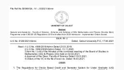
File Ref.No.50068/GA - IV - J3/2021/Admn, , UNIVERSITY OF CALICUT, Abstract, , General and Academic - Faculty of Science - Scheme and Syllabus of BSc Mathematics and Physics (Double Main), Programme under CBCSS UG Regulations 2019 with effect from 2020 Admission - Implemented- Orders Issued., G & A - IV - J, , U.O.No. 8128/2021/Admn, , Dated, Calicut University.P.O, 17.08.2021, , Read:-1.U.O.No. 4368/2019/Admn Dated 23.03.2019., 2.U.O.No. 10662/2020/Admn Dated, 13.11.2020., 3.Item No.1.(viii) of the Minutes of the combined meeting of the Board of Studies in, Mathematics (UG) & Physics (UG) held on 02.02.2021., 4.Approval of the Dean, Faculty of Science Dated 15.03.2021., 5.Orders of the VC in the file of even no. Dated 18.03.2021., ORDER, , 1. The Regulations for Choice Based Credit and Semester System for Under Graduate (UG), Curriculum-2019 (CBCSS UG Regulations 2019) for all UG Programmes under CBCSS-Regular, and SDE/Private Registration w.e.f. 2019 admission has been implemented vide paper read first, above and same has been modified, vide paper read second above., , 2. The combined online meeting of Boards of Studies in Mathematics UG and Physics UG held on, 02.02.2021 has approved the Scheme and Syllabus of B Sc Mathematics and Physics (Double, Main) Programme in tune with the, CBCSS UG-2019 Regulations with effect from, 2020 Admission, vide paper read third above., , 3. The Dean, Faculty of Science has approved the minutes of the combined online meeting of the, Boards of Studies in Mathematics UG and Physics UG held on 02.02.2021, vide paper read, fourth above., , 4. Under these circumstances, considering the urgency, the Vice Chancellor has accorded, , sanction to implement the Scheme and Syllabus of B Sc Mathematics and Physics (Double, Main) Programme in accordance with the CBCSS UG Regulations 2019, in the University with, effect from 2020 Admission, subject to ratification by the Academic Council., , 5. The Scheme and Syllabus of B Sc Mathematics and Physics (Double Main) Programme in, accordance with CBCSS UG Regulations 2019, is therefore implemented in the University with, effect from 2020 Admission., , 6. Orders are issued accordingly. (Syllabus appended), Ajitha P.P, Joint Registrar, To, , The Principals of all Affiliated Colleges, Copy to: PS to VC/PA to PVC/ PA to Registrar/PA to CE/JCE I/JCE IV/DR, DOA/DR,CDC/EX, and EG Branches/GA-I-F Section/CHMK Library/Information Centres/SF/DF/FC, Forwarded / By Order, Section Officer
Page 3 :
Syllabus structure, The following courses are compulsory for the BSc Mathematics and Physics Double main, programme., , PHY 2B22, PHY 2B23, MTS 2B22, E02, , 3, , A11, A12, PHY 3B24, PHY 3B25, MTS 3B23, MTS 3B24, E03, , 1, , Exam dur.(Hrs), , 2, , Total, , A03, A04, A08, , External, , MTS 1B21, E01, , Internal, , PHY 1B21, , Credits, , 1, , Name of the course, Common Course I – English, Common Course II – English, Common Course : Additional, Language I, Mechanics I, Practical I, Basic Calculus, Environment Studies, TOTAL, Common Course I – English, Common Course II – English, Common Course : Additional, Language I, Mechanics II, Practical I, Advanced Calculus, Disaster Management, TOTAL, General Course, General Course, Electrodynamics, Thermodynamics, Practical II, Abstract Algebra, Multivariable Calculus, Human Rights or Intellectual, Property Rights or Consumer, protection, TOTAL, , No of contact, hours/Week, , Code, A01, A02, A07, , Total No, Contact hours, , Semester, , Max. Marks, , 64, 80, 64, , 4, 5, 4, , 3, 3, 4, , 15, 15, 20, , 60, 60, 80, , 75, 75, 100, , 2, 2, 2.5, , 32, 64, 96, , 2, 4, 6, , 15, 20, , 60, 80, , 75, 100, , 2, 2.5, , 80, 64, 64, , 25, 5, 4, 4, , 2, 4, 4**, 16, 4, 4, 4, , 20, 20, 20, , 80, 80, 80, , 425, 100, 100, 100, , 2.5, 2.5, 2.5, , 32, 64, 96, , 2, 4, 6, , 15, 15, 20, , 60, 60, 80, , 75, 75, 100, , 2, 3, 2.5, , 80, 80, 48, 48, 32, 64, 48, , 25, 5, 5, 3, 3, 2, 4, 3, , 2, 2, 4, 4**, 20, 4, 4, 3, 3, 3, 3, 4**, , 80, 80, 60, 60, 60, 60, , 550, 100, 100, 75, 75, 75, 75, , 2.5, 2.5, 2, 2, 2, 2, , 25, , 20, , 20, 20, 15, 15, 15, 15, , 500
Page 4 :
2, , PHY 5B29, PHY 5B30, , MTS 5B27, MTS 5B28, , PHY 6B31, , 6, , PHY, PHY, PHY, PHY, MTS, MTS, MTS, , 6B32, 6B33, 6B34, 6B35, 6B29, 6B30, 6B31, , Exam dur.(Hrs), , 5, , Total, , PHY 5B28, , External, , MTS 4B25, MTS 4B26, E04, , Internal, , PHY 4B27, , Credits, , 4, , Name of the course, General Course, General Course, Statistical Physics, Solid, State Physics, Spectroscopy, and Photonics, Electronics (Analog and, Digital), Practical III, Differential Equations, Number Theory, Gender studies or, Gerontology, TOTAL, Relativistic Mechanics and, Astrophysics, Optics, Quantum Mechanics, Practical II, Practical III, Complex Analysis, Real Analysis - I, Open Course (offered by, Other Departments), TOTAL, Nuclear Physics and Particle, Physics, Elective (Physics Core), Practical II, Practical III, Project + Tour Report, Linear Algebra, Real Analysis - II, Elective (Mathematics Core), TOTAL, Grand Total, , No of contact, hours/Week, , Code, A13, A14, PHY 4B26, , Total No, Contact hours, , Semester, , Max. Marks, , 80, 80, 48, , 5, 5, 3, , 4, 4, 3, , 20, 20, 15, , 80, 80, 60, , 100, 100, 75, , 2.5, 2.5, 2, , 48, , 3, , 3, , 15, , 60, , 75, , 2, , 32, 64, 48, , 2, 4, 3, , 3, 3, 4**, , 15, 15, , 60, 60, , 75, 75, , 2, 2, , 48, , 25, 3, , 20, 3, , 15, , 60, , 500, 75, , 2, , 48, 48, 32, 32, 80, 64, 48, , 3, 3, 2, 2, 5, 4, 3, , 3, 3, 5, 4, 3, , 15, 15, 20, 20, 15, , 60, 60, 80, 80, 60, , 75, 75, 100, 100, 75, , 2, 2, 2.5, 2.5, 2, , 64, , 25, 4, , 21, 3, , 15, , 60, , 500, 75, , 2, , 3, 2, 2, 2, 5, 4, 3, 25, , 3, 2, 2, 2+1, 4, 3, 3, 23, 120, , 15, 15, 15, 15, 20, 15, 15, , 60, 60, 60, 60, 80, 60, 60, , 48, 32, 32, 32, 80, 64, 48, , 75, 75, 75, 75, 100, 75, 75, 625, 3100, , 2, 3, 3, 2.5, 2, 2, , Tour report shall be evaluated with Practical III, *Credit for practical / project to be awarded only at the end of Semester 2 and Semester 6., **Mandatory audit courses for the program, but not counted for the calculation of SGPA or CGPA., Student can attain only pass (Grade P) for these courses
Page 5 :
3, , Elective Courses (Mathematics Core), One of the following three courses can be offered in the sixth semester as an elective course, under Mathematics Core. (Code MTS 6B31(E01), MTS 6B31(E02) and MTS 6B31(E03))., , Credits, , Internal, , External, , Total Marks, , Exam dur.(in Hrs), , MTS 6B31(E03), , Hours/week, , 3, , 6, 6, , 48, 48, , 3, 3, , 3, 3, , 15, 15, , 60, 60, , 75, 75, , 2, 2, , 6, , 48, , 3, , 3, , 15, , 60, , 75, , 2, , Contact Hours, , MTS 6B31(E01), MTS 6B31(E02), , Total No. of, , Course Code, , 1, 2, , Course Title, Numerical Analysis, Introduction to, Geometry, Linear Programming, , Semester, , Sl. No, , Max. Marks, , Elective Courses (Physics Core), One of the following three courses can be offered in the sixth semester as an elective course, under Physics Core (Code PHY 6B32(EL1), PHY 6B32(EL2) and PHY 6B32(EL3)))., , Credits, , Internal, , External, , Total Marks, , Exam dur.(in Hrs), , PHY 6B32(EL3), , Hours/week, , 3, , 6, 6, , 48, 48, , 3, 3, , 3, 3, , 15, 15, , 60, 60, , 75, 75, , 2, 2, , 6, , 48, , 3, , 3, , 15, , 60, , 75, , 2, , Contact Hours, , PHY 6B32(EL1), PHY 6B32(EL2), , Total No. of, , Course Code, , 1, 2, , Course Title, Biomedical Physics, Nanoscience and, Technology, Materials Science, , Semester, , Sl. No, , Max. Marks
Page 6 :
4, , Open Courses, One of the following four courses (MTS 5D01, MTS 5D02, MTS 5D03 and MTS 5D04) can be, offered (under Mathematics Core) in the fifth semester as an open course for the students, not having Mathematics as Core Course and Mathematics and Physics double main programme., The syllabus of these courses were attached in the syllabus of B.Sc. Mathematics programme., , Internal, , External, , Total, , Unty. exam, Dur. (Hrs), , MTS 5D03, MTS 5D04, , Credits, , 3, 4, , Name of the course, Applied Calculus, Discrete Mathematics for Basic, and Applied Sciences, Linear Mathematical Models, Mathematics for Decision, Making, , No of contact, hours/Week, , 1, 2, , Code, MTS 5D01, MTS 5D02, , Semester, , Sl. No, , Max. Marks, , 5, 5, , 3, 3, , 3, 3, , 15, 15, , 60, 60, , 75, 75, , 2, 2, , 5, 5, , 3, 3, , 3, 3, , 15, 15, , 60, 60, , 75, 75, , 2, 2, , Credit Distribution, Semester, , 1, 2, 3, 4, 5, 6, Total, , Common course, English Additional, Language, 3+3, 4, 4+4, 4, 14, 8, , General, Core course, Course Mathematics Physics, , 4+4, 4+4, 16, , 4, 4, 3+3, 3+3, 5+4, 4+3+3, 39, , Open Project, course +, Total, Tour, 2, 16, 2+2*, 20, 3+3, 20, 3+3, 20, 3+3+3, 3, 21, 3+3+2*+2* 2+1, 23, 37, 3, 3, 120, , Project and Tour should be offered under Physics Core. Hence total credit under Physics, core is 40., *Practical, Tour report to be evaluated with Practical Paper III
Page 7 :
5, , Scheme of Evaluation, The evaluation scheme for each course shall contain two parts: internal evaluation and external evaluation., , Internal Evaluation, 20% of the total marks in each course are for internal evaluation. The colleges shall send only the, marks obtained for internal examination to the university., , Components of Internal Evaluation, Sl, No, 1, 2, 3, 4, , Components, Class Room Participation, (Attendance), Assignment, Seminar, Test paper, Total, , Marks (For Courses with, Maximum Marks 75), 3, , Marks (For Courses, with Max. Marks 100), 4, , 3, 3, 6, 15, , 4, 4, 8, 20, , a) Percentage of Class Room Participation (Attendance) in a Semester and, Eligible Internal Marks, % of Class Room Participation (Attendance), 50% ≤ CRP < 75%, 75% ≤ CRP < 85%, 85% and above, , Out of 3 (Maximum internal, marks is 15), 1, 2, 3, , Out of 4 (Maximum internal, marks is 20), 1, 2, 4, , CRP means % of class room participation (Attendance), b) Percentage of Marks in a Test Paper and Eligible Internal Marks, Range of Marks in test paper (TP), Less than 35%, 35% ≤ T P < 45%, 45% ≤ T P < 55%, 55% ≤ T P < 65%, 65% ≤ T P < 85%, 85% ≤ T P ≤ 100%, , Out of 6 (Maximum, internal marks is 15), 1, 2, 3, 4, 5, 6, , Out of 8 (Maximum, internal marks is 20), 1, 2, 3, 4, 6, 8
Page 8 :
6, , Pattern of Question Paper for University Examinations, For Courses with Maximum, External Marks 80 (2.5 Hrs), Short answer type Ceiling - 25, carries 2 marks each, - 15 questions, Paragraph/Problem Ceiling - 35, type carries 5 marks, each - 8 questions, Essay type carries 2 × 10 = 20, 10 marks (2 out of 4), 80, , Section A, , Section B, , Section C, Total, , For Courses with Maximum, External Marks 60 (2 Hrs), Short answer type Ceiling - 20, carries 2 marks each, - 12 questions, Paragraph/Problem Ceiling - 30, type carries 5 marks, each - 7 questions, Essay type carries 1 × 10 = 10, 10 marks (1 out of 2), 60, , *Questions are to be evenly distributed over the entire syllabus., , Physics Core Course : Practical Evaluation Scheme (60 Marks), Internal (15), Items, Marks, Record, , 3, , Regularity, in doing the, experiment, Attendance, Test 1, , 3, , Test 2, , 3, , Total, , 3, 3, , 15, , External (60), Items, , Marks, , Record with 20 experiments Maximum 1/2 mark for each experiment, Formulae, Theory, Principle/, Program, , 10, , Marks for, Python, Programming, 10, , 15, , 15, , Adjustments & setting/ Algorithm, Tabulation, Observation and, performance/Execution, Calculation, result, graph, unit/, Result, Viva, Total, , 10, 14, , 12, 14, , 8, , 6, , 3, 60, , 3, 60
Page 9 :
., , SYLLABUS, PHYSICS CORE COURSES
Page 10 :
8, , Physics Core Courses, Credit, Mark and Hour distribution, , 2, , 3, , Internal, , External, , Total, , Exam.dur.(Hrs), , 1, , PHY 1B21, , Mechanics I, , 32, , 2, , 2, , 15, , 60, , 75, , 2, , Practical I, , 64, , 4, , -, , -, , -, , -, , *, , hours/Week, Credits, , Name of the course, , Contact hours, No of contact, , Code, , Total No, , 1, , Sl. No., , Semester, , Max. Marks, , 2, , PHY 2B22, , Mechanics II, , 32, , 2, , 2, , 15, , 60, , 75, , 2, , 3, , PHY 2B23, , Practical I, , 64, , 4, , 2, , 15, , 60, , 75, , 3, , 4, , PHY 3B24, , Electrodynamics, , 48, , 3, , 3, , 15, , 60, , 75, , 2, , 5, , PHY 3B25, , Thermodynamics, , 48, , 3, , 3, , 15, , 60, , 75, , 2, , Practical II, , 32, , 2, , -, , -, , -, , -, , *, , Statistical Physics, Solid State, , 48, , 3, , 3, , 15, , 60, , 75, , 2, , Electronics (Analog & Digital), , 48, , 3, , 3, , 15, , 60, , 75, , 2, , Practical III, , 32, , 2, , -, , -, , -, , -, , *, , Relativistic Mechanics and, , 48, , 3, , 3, , 15, , 60, , 75, , 2, , Optics, , 48, , 3, , 3, , 15, , 60, , 75, , 2, , Quantum Mechanics, , 48, , 3, , 3, , 15, , 60, , 75, , 2, , Practical II, , 32, , 2, , -, , -, , -, , -, , *, , Practical III, , 32, , 2, , -, , -, , -, , -, , *, , Nuclear Physics and Particle, , 64, , 4, , 3, , 15, , 60, , 75, , 2, , 48, , 3, , 3, , 15, , 60, , 75, , 2, , 6, , PHY 4B26, , 4, , Physics, Spectroscopy Photonics, 7, 8, , PHY 4B27, PHY 5B28, , Astrophysics, 5, , 9, , PHY 5B29, , 10 PHY 5B30, , 11 PHY 6B31, , Physics, 12 PHY 6B32, , Elective (Physics Core), EL1–Biomedical Physics, , 6, , EL2–Nanoscience & Technology, EL3–Materials Science, 13 PHY 6B33, , Practical II, , 32, , 2, , 2, , 15, , 60, , 75, , 3, , 14 PHY 6B34, , Practical III, , 32, , 2, , 2, , 15, , 60, , 75, , 3, , 15 PHY 6B35, , Project + Tour Report, , 32, , 2, , 2+1, , 15, , 60, , 75, , -, , Grand Total, , 40, , Tour report shall be evaluated with Practical III, *Credit for practical / project to be awarded only at the end of Semester 2 and Semester 6.
Page 11 :
9, , Programme Specific Outcomes Under Physics Core, , PSO1 :, , Understand the basic concepts of fundamentals of mechanics, properties of matter and electrodynamics, , PSO2 :, , Understand the theoretical basis of quantum mechanics, relativistic physics, nuclear physics,, optics, spectroscopy, solid state physics, astrophysics, statistical physics, photonics and thermodynamics, , PSO3 :, , Understand and apply the concepts of electronics in the designing of different analog and digital, circuits, , PSO4 :, , Understand the basics of computer programming and numerical analysis, , PSO5 :, , Apply and verify theoretical concepts through laboratory experiments, , Abbreviations used, CL – Cognitive level;, U – understand;, Ap – apply;, An – analyze;, C – create, KC – Knowledge category;, C – conceptual;, F – factual;, P – procedural
Page 12 :
10, , SEMESTER – 1; Physics Core Course 1, PHY 1B21 : MECHANICS – I, 2 Hours/Week, , 2 Credits, , Course Outcome, , 75 Marks[Int: 15 + Ext : 60], PSO, , CL, , KC, , Class Sessions, Allotted, , C01, , Understand and apply the basic concepts of, , PSO1, , Ap, , C,P, , 14, , PSO1, , Ap, , C,P, , 8, , PSO1, , Ap, , C,P, , 10, , Newtonian Mechanics to Physical Systems, C02, , Understand and apply the basic idea of workenergy theorem to physical systems, , C03, , Understand and apply the rotational dynamics, of rigid bodies, , Unit I – Newton’s Laws, , (14 hrs), , Newton’s First Law, Second Law and Third Law – Astronauts in space : Inertial systems and fictitious, forces – Standards and units – Some applications of Newton’s laws – The astronauts’ tug of war, Freight, train, Constraints, Block on string, The whirling block, The conical pendulum – The everyday forces, of physics – Gravity and Weight; Gravitational force of a sphere; Turtle in an elevator; Gravitational, field – Electrostatic force – Contact forces; Block and string; Dangling rope; Whirling rope; Pulleys;, Tension and Atomic forces; Normal force; Friction; Block and wedge with friction; Viscosity – Linear, restoring force; Spring and block : The equation for simple harmonic motion; Spring and gun :, Illustration of initial conditions – Dynamics of a system of particles – The Bola – Centre of mass –, Drum major’s baton – Centre of mass motion – Conservation of momentum – Spring Gun recoil, [Sections 2.1 to 2.5, 3.1 to 3.3 of An Introduction to Mechanics (1stEdn.) by Daniel Kleppner and, Robert J. Kolenkow], , Unit II – Work and Energy, , (8 hrs), , Integrating the equation of motion in one dimension – Mass thrown upward in a uniform gravitational, field; Solving the equation of simple harmonic motion – Work-energy theorem in one dimension –, Vertical motion in an inverse square filed – Integrating the equation of motion in several dimensions, – Work-energy theorem – Conical pendulum; Escape velocity – Applying the work-energy theorem –, Work done by a uniform force; Work done by a central force; Potential energy – Potential energy of a
Page 13 :
11, , uniform force field; Potential energy of an inverse square force – What potential energy tells us about, force – Stability – Energy diagrams – Small oscillations in a bound system – Molecular vibrations –, Nonconservative forces – General law of conservation of energy – Power, [Sections 4.1 to 4.13 of An Introduction to Mechanics (1stEdn.) by Daniel Kleppner and Robert, J. Kolenkow. The problems in chapter 5 should be discussed with this.], , Unit III – Angular Momentum, , (10 hrs), , Angular momentum of a particle – Angular momentum of a sliding block; Angular momentum of the, conical pendulum – Torque – Central force motion and the law of equal areas – Torque on a sliding, block; Torque on the conical pendulum; Torque due to gravity – Angular momentum and fixed axis, rotation – Moments of inertia of some simple objects – The parallel axis theorem – Dynamics of, pure rotation about an axis – Atwood’s machine with a massive pulley – The simple pendulum – The, physical pendulum – Motion involving both translation and rotation – Angular momentum of a rolling, wheel – Drum rolling down a plane – Work-energy theorem for a rigid body – Drum rolling down a, plane : energy method – The vector nature of angular velocity and angular momentum – Rotation, through finite angles – Rotation in the xy-plane – Vector nature of angular velocity – Conservation of, angular momentum, [Sections 6.1 to 6.7, 7.1, 7.2 and 7.5 of An Introduction to Mechanics (1stEdn.) by Daniel Kleppner, and Robert J. Kolenkow], , Books of Study :, 1. An Introduction to Mechanics, 1st Edn. – Daniel Kleppner and Robert J. Kolenkow – McGrawHill, , Reference Books :, 1. Berkeley Physics Course : Vol.1 : Mechanics, 2ndEdn. – Kittelet al. – McGraw-Hill, Mark Distribution for Setting Question Paper, , Unit/Chapter, , Title, , Marks, , 1, , Newton’s laws, , 36, , 2, , Work and Energy, , 18, , 3, , Angular Momentum, , 25, , Total Marks*, , 79, , *Total marks include that for choice of questions in sections A, B and C in the question paper.
Page 14 :
12, , SEMESTER – 2; Physics Core Course 2, PHY 2B22 : MECHANICS – II, 2 Hours/Week, , 2 Credits, , Course Outcome, , 75 Marks[Int: 15 + Ext : 60], , PSO, , CL, , KC, , Class Sessions, Allotted, , C01, , Understand the features of non-inertial systems, , PSO1, , U, , C, , 7, , PSO1, , An, , C,P, , 9, , PSO1, , U, , C, , 7, , PSO1, , An, , C,P, , 9, , and fictitious forces, C02, , Understand and analyze the features of central, forces with respect to planetary forces, , C03, , Understand the basic ideas of Harmonic, oscillator, , C04, , Understand and analyze the basic concepts of, wave motion, , Unit I – Noninertial Systems and Fictitious Forces, , (7 hrs), , Galilean transformations – Uniformly accelerating systems – The apparent force of gravity – Pendulum, in an accelerating car – The principle of equivalence – The driving force of the tides – Physics in a, rotating coordinate system – Time derivatives and rotating coordinates – Acceleration relative to, rotating coordinates – The apparent force in a rotating coordinate system – The Coriolis force –, Deflection of a falling mass – Motion on the rotating earth – Weather systems – Foucault’s pendulum, [Sections 8.1 to 8.5 of An Introduction to Mechanics (1st Edn.) by Daniel Kleppner and Robert, J. Kolenkow], , Unit II – Central Force Motion, , (9 hrs), , Central force motion as a one-body problem – General properties of central force motion – Motion, is confined to a plane – Energy and angular momentum are constants of the motion – The law of, equal areas – Finding the motion in real problems – The energy equation and energy diagrams –, Noninteracting particles – Planetary motion – Hyperbolic orbits – Satellite orbit – Kepler’s laws –, The law of periods – Properties of the ellipse, [Sections 9.1 to 9.7 of An Introduction to Mechanics (1st Edn.) by Daniel Kleppner and Robert, J. Kolenkow]
Page 15 :
13, , Unit III – Harmonic Oscillator, , (7 hrs), , Introduction and review – Standard form of the solution – Nomenclature – Initial conditions and the, frictionless harmonic oscillator – Energy considerations – Time average values – Average energy –, Damped harmonic oscillator – Energy and Q-factor – Q factor of two simple oscillators – Graphical, analysis of a damped oscillator – Solution of the equation of motion for the undriven damped oscillator, – Forced harmonic oscillator – Undamped forced oscillator – Resonance, [Sections 10.1 to 10.3 (except the topic, The Forced Damped Harmonic Oscillator) and Note 10.1, of An Introduction to Mechanics (1stEdn.) by Daniel Kleppner and Robert J. Kolenkow], , Unit IV – Waves, , (9 hrs), , What is a wave? – Normal modes and travelling waves – Progressive waves in one direction – Wave, speeds in specific media – Superposition – Wave pulses – Motion of wave pulses of constant shape –, Superposition of wave pulses – Dispersion; Phase and Group Velocities – Energy in a mechanical wave, – Transport of energy by a wave – Momentum flow and mechanical radiation pressure – Waves in two, and three dimensions, [Chapter 7 – Progressive Waves (except the topic, The Phenomenon of Cut-off)of Vibrations and, Waves by A. P. French], , Books of Study :, 1. An Introduction to Mechanics, 1stEdn. – Daniel Kleppner and Robert J. Kolenkow – McGrawHill, 2. Vibrations and Waves – A. P. French – The M.I.T. Introductory Physics Series – CBS Publishers, & Distributors, , Reference Books :, 1. Berkeley Physics Course : Vol.1 : Mechanics, 2nd Edn. – Kittel et. al. – McGraw-Hill, Mark Distribution for Setting Question Paper, , Unit/Chapter, , Title, , Marks, , 1, , Non-inertial systems and fictitious forces, , 18, , 2, , Central Force Motion, , 22, , 3, , Harmonic Oscillator, , 18, , 4, , Waves, , 21, Total Marks*, , 79, , *Total marks include that for choice of questions in sections A, B and C in the question paper.
Page 16 :
14, , SEMESTER – 3; Physics Core Course 4, PHY 3B24: ELECTRODYNAMICS, 3 Hours/Week, , 3 Credits, , Course Outcome, , 75 Marks[Int: 15 + Ext : 60], PSO, , CL, , KC, , Class Sessions, Allotted, , CO1, , Understand and analyze the electrostatic prop-, , PSO1, , An, , C,P, , 12, , PSO1, , U, , C, P, , 8, , PSO1, , U, , C,P, , 8, , PSO1, , U, , C,P, , 8, , PSO1, , U, , C,P, , 12, , erties of physical systems, CO2, , Understand the mechanism of electric field in, matter, , CO3, , Understand and analyze the magnetic properties, of physical systems, , CO4, , Understand the mechanism of magnetic field in, matter, , CO5, , Understand the basic concepts of electrodynamics and electromagnetic waves and analyze the, properties of electromagnetic waves, , Unit 1 – Electrostatics, , (12 hrs), , Electrostatic field – Coulomb’s law, Electric field, Continuous charge distributions – Divergence and, curl of electrostatic field, Field lines and Gauss’s law, The divergence of E, Applications of Gauss law,, Curl of E – Electric potential – Comments on potential, Poisson’s equation and Laplace’s equation,, The potential of a localized charge distribution, Electrostatic boundary conditions – Work and energy, in electrostatics, The work done in moving a charge, The energy of point charge distribution., [Sections 2.1 to 2.4.2 of Introduction to Electrodynamics by David J Griffiths. Additional problems, should be done from chapters 1, 2 and 3 of Berkeley Physics Course: Vol.2: Electricity and Magnetism, (2nd Edn.) by Edward M Purcell.], , Unit 2 – Electric fields in matter, , (8 hrs), , Polarization – Dielectrics, Induced dipoles, Alignment of polar molecules, Polarization – The field, of a polarized object, Bound charges, Physical interpretation of bound charges, The field inside a, dielectric – The electric displacement – Gauss’s law in presence of dielectrics, Boundary conditions
Page 17 :
15, , for D – Linear dielectrics, Susceptibility, Permittivity, Dielectric constant, Boundary value problems, with linear dielectrics, Energy in dielectric systems, Forces on dielectrics., [Sections 4.1 to 4.4 of Introduction to Electrodynamics (4th Edn.) by David J Griffiths. Additional, problems should be done from chapter 10 of Berkeley Physics Course: Vol.2: Electricity and Magnetism, (2nd Edn.) by Edward M Purcell.], , Unit 3 – Magnetostatics, , (8 hrs), , The Lorentz force law – Magnetic fields, Magnetic forces, cyclotron motion, cycloid motion, Currents,, Linear, Surface and Volume current density – Biot -Savart law, The magnetic field of steady current, – Divergence and curl of B, Straight line currents, Applications of Ampere’s law, Magnetic vector, potential, Vector potential, Magnetostatic boundary conditions., [Sections 5.1 to 5.4.2 of Introduction to Electrodynamics (4th Edn.) by David J Griffiths. Additional problems should be done from chapter 6 of Berkeley Physics Course: Vol.2: Electricity and, Magnetism (2nd Edn.) by Edward M Purcell.], , Unit 4 – Magnetostatic fields in matter, , (8 hrs), , Magnetization – Diamagnets, Paramagnets and Ferromagnets, Torques and forces on magnetic dipoles,, Effect of a magnetic field on atomic orbits, Magnetization – Field of a magnetised object, Bound, Currents, Physical interpretation of bound currents, Magnetic field inside matter – Auxiliary field H,, Ampere’s law in magnetized materials, Boundary conditions – Linear and nonlinear media, Magnetic, susceptibility and permeability, Ferromagnetism., [Sections 6.1 to 6.4 of Introduction to Electrodynamics (4th Edn.) by David J Griffiths. Additional, problems should be done from chapter 11 of Berkeley Physics Course: Vol.2: Electricity and Magnetism, (2nd Edn.) by Edward M Purcell.], , Unit 5 – Electrodynamics and Electromagnetic Waves, , (12 hrs), , Electromotive force – Ohm’s law, electromotive force, motional emf – Electromagnetic induction –, Faraday’s law, induced electric field, inductance, energy in magnetic fields – Maxwell’s equations, – Electrodynamics before Maxwell, Maxwell’s modification of Ampere’s law, Maxwell’s equations,, Magnetic charge, Maxwell’s equations inside matter, Boundary conditions – Continuity equation –, Poynting’s theorem., Electromagnetic waves in vacuum, Wave equation for E and B, monochromatic plane waves in, vacuum, energy, and momentum of E.M. waves, Poynting vector., [Sections 7.1 to 7.3, 8.1 and 9.2 to 9.3.1 of Introduction to Electrodynamics by David J Griffiths.
Page 18 :
16, , Additional problems should be done from chapter 7 of Berkeley Physics Course: Vol.2: Electricity and, Magnetism (2nd Edn.) by Edward M Purcell.], , Books of Study :, 1. Introduction to Electrodynamics, 4th Edn. – David J Griffiths – Prentice Hall India Learning, Pvt. Ltd., 2. Berkeley Physics Course: Vol.2: Electricity and Magnetism, 2nd Edn. – Edward M. Purcell –, McGraw-Hill, , Reference Books :, 1. Electricity and magnetism by Arthur F Kip, 2. Physics Vol. II by Resnick and Halliday, 3. Electricity and Magnetism-Hugh D Young and Roger A Freedman, 4. Electricity and Magnetism by D.N Vasudeva (12threvised edition), 5. Electromagnetics by Edminister – Schaum’s Outline – Tata McGraw Hill, 6. NPTEL video lectures available online, Mark Distribution for Setting Question Paper, , Unit/Chapter, , Title, , Marks, , 1, , Electrostatics, , 20, , 2, , Electric fields in matter, , 13, , 3, , Magnetostatics, , 13, , 4, , Magnetostatic fields in matter, , 13, , 5, , Electrodynamics and Electromagnetic waves, , 20, , Total Marks*, , 79, , *Total marks include that for choice of questions in sections A, B and C in the question paper.
Page 19 :
17, , SEMESTER – 3; Physics Core Course 5, PHY 3B25: THERMODYNAMICS, 3 Hours/Week, , 3 Credits, , Course Outcome, , 75 Marks[Int: 15 + Ext : 60], PSO, , CL, , KC, , Class Sessions, Allotted, , CO1, , Understand the zero and first laws of thermody-, , PSO2, , U, , C, , 12, , PSO2, , U, , C, , 7, , PSO2, , U, , C, P, , 11, , namics, CO2, , Understand the thermodynamics description of, the ideal gas, , CO3, , Understand the second law of thermodynamics, and its applications, , CO4, , Understand the basic ideas of entropy, , PSO2, , U, , C, , 7, , CO5, , Understand the concepts of thermodynamic po-, , PSO2, , U, , C, , 11, , tentials and phase transitions, , Unit 1 – Zeroth Law and First Law of Thermodynamics, , (12 hrs), , Macroscopic point of view – Microscopic point of view – Macroscopic versus Microscopic points of, view – Scope of Thermodynamics – Thermal equilibrium and Zeroth Law – Concept of temperature, – Ideal-Gas temperature – Thermodynamic equilibrium – Equation of state – Hydrostatic systems –, Intensive and extensive coordinates – Work – Quasi-static process – Work in changing the volume of, a hydrostatic system – PV diagram – Hydrostatic work depends on the path – Calculation of work for, quasi-static processes – Work and Heat – Adiabatic work – Internal energy function – Mathematical, formulation of First Law – Concept of Heat – Differential form of the First Law – Heat capacity –, Specific heat of water; the Calorie – Quasi-static flow of heat; Heat reservoir, [Sections 1.1 to 1.6, 1.10, 2.1 to 2.3, 2.10, 3.1 to 3.6 and 4.1 to 4.8, 4.10 of Heat and Thermodynamics by Zemansky and Dittman], , Unit 2 – Ideal Gas, , (7 hrs), , Equation of state of a gas – Internal energy of a real gas – Ideal gas – Experimental determination of, heat capacities – Quasi-static adiabatic process – The microscopic point of view – Kinetic theory of, the ideal gas
Page 20 :
18, , [Sections 5.1 to 5.5, 5.8 and 5.9 of Heat and Thermodynamics by Zemansky and Dittman], , Unit 3 – Second Law of Thermodynamics, , (11 hrs), , Conversion of work into heat and vice versa – Heat engine; Kelvin-Planck statement of the Second Law, – Refrigerator; Clausius’ statement of the Second Law – Equivalence of Kelvin-Planck and Clausius, statements – Reversibility and Irreversibility – Conditions for reversibility – Carnot engine and Carnot, cycle – Carnot refrigerator – Carnot’s Theorem and corollary – Thermodynamic temperature scale –, Absolute zero and Carnot efficiency – Equality of ideal-gas and thermodynamic temperatures, [Sections 6.1, 6.6 to 6.9, 6.14, 7.1 and 7.3 to 7.7 of Heat and Thermodynamics by Zemansky and, Dittman], , Unit 4 – Entropy, , (7 hrs), , Reversible part of the Second Law – Entropy – Entropy of the ideal gas – TS diagram – Entropy and, reversibility – Entropy and irreversibility – Irreversible part of the Second Law – Heat and entropy, in irreversible processes – Principle of increase of entropy – Applications of the Entropy Principle –, Entropy and disorder – Exact differentials, [Sections 8.1, 8.2, 8.4 to 8.9, 8.11 to 8.14 of Heat and Thermodynamics by Zemansky and Dittman], , Unit 5 – Thermodynamic Potentials and Phase Transitions (11 hrs), Characteristic functions – Enthalpy – Joule-Thomson expansion – Helmholtz and Gibbs functions –, Condition for an exact differential – Maxwell’s relations – TdS equations – PV diagram for a pure, substance – PT diagram for a pure substance; Phase diagram – First-order phase transitions and, Clausius-Clapeyron equation – Clausius-Clapeyron equation and phase diagrams, [Sections 10.1 to 10.6, 9.1, 9.2, 11.3 and 11.4 of Heat and Thermodynamics by Zemansky and, Dittman], , Books of Study :, 1. Heat and Thermodynamics, 7thEdn. – Mark W. Zemansky and Richard H. Dittman – McGrawHill, , Reference Books :, 1. Classical and Statistical Thermodynamics – Ashley H. Carter – Pearson, 2012
Page 21 :
19, , 2. Basic Thermodynamics – Evelyn Guha – Narosa, 2002, 3. Heat and Thermodynamics – D. S. Mathur – S. Chand Publishers, 2008, 4. NPTEL video lectures available online, Mark Distribution for Setting Question Paper, , Unit/Chapter, , Title, , Marks, , 1, , Zeroth Law and First Law of Thermodynamics, , 20, , 2, , Ideal Gas, , 12, , 3, , Second Law of Thermodynamic, , 18, , 4, , Entropy, , 12, , 5, , Thermodynamic Potentials and Phase Transitions, , 17, , Total Marks*, , 79, , *Total marks include that for choice of questions in sections A, B and C in the question paper.
Page 22 :
20, , SEMESTER – 4; Physics Core Course 6, PHY 4B26 : STATISTICAL PHYSICS, SOLID STATE, PHYSICS, SPECTROSCOPY & PHOTONICS, 3 Hours/Week, , 3 Credits, , Course Outcome, , 75 Marks[Int: 15 + Ext : 60], , PSO, , CL, , KC, , Class Sessions, Allotted, , CO1, , Understand the basic principles of statistical, , PSO2, , U, , C, , 14, , PSO2, , U, , C, , 13, , physics and its applications, CO2, , Understand the basic aspects of crystallography, in solid state physics, , CO3, , Understand the basic elements of spectroscopy, , PSO2, , U, , C, , 3, , CO4, , Understand the basics ideas of microwave and, , PSO2, , U, , C, , 11, , PSO2, , U, , C, , 7, , infra red spectroscopy, CO5, , Understand the fundamental ideas of photonics, , Unit 1 – Statistical Physics, , (14 hrs), , Statistical Analysis – Classical versus quantum statistics – Distribution of molecular speeds – MaxwellBoltzmann distribution – Quantum Statistics – Applications of Bose-Einstein statistics – Blackbody, radiation – Applications of Fermi-Dirac statistics, [Sections 10.1 to 10.7 of Modern Physics by Kenneth Krane], , Unit 2 – Solid State Physics, , (13 hrs), , Lattice Points and Space Lattice-Basis and crystal structure, unit cells and lattice Parameters, Unit, cells versus primitive cells, Crystal systems, Crystal symmetry, Bravais space lattices – Metallic crystal structures – simple cubic, body-centered cubic, face-centered cubic and hexagonal closed packed, structure – Other crystal structures – Diamond, Zinc sulphide, Sodium chloride, Caesium chloride –, Directions, Planes and Miller indices – Important features of Miller indices – Important planes and, directions, distribution of atoms and separation between lattice planes in a cubic crystal – X-Ray, diffraction – Bragg’s law – Bragg’s X-ray spectrometer – Powder crystal method, [Sections 4.1 to 4.7, 4.14 to 4.22 and 5.7 to 5.10 of Solid State Physics by S.O. Pillai]
Page 23 :
21, , Unit 3 – Basic Elements of Spectroscopy, , (3 hrs), , Quantization of Energy-Regions of Spectrum-Representation of Spectra-Basic Elements of Practical, Spectroscopy-Signal to Noise Ratio-Resolving Power-Width and Intensity of Spectral Transitions, [Sections 1.2 to 1.7 of Fundamentals of Molecular Spectroscopy by Banwell and McCash], , Unit 4, Microwave Spectroscopy, , (5 hrs), , Rotation of molecules – Rotational spectra – Rigid diatomic molecules – Bond length of CO molecule, – Intensities of spectral lines, [Sections 2.1 to 2.3.2 of Fundamentals of Molecular Spectroscopy by Banwell and McCash], Infra Red Spectroscopy & Raman Spectroscopy, , (6 hrs), , Energy of a diatomic molecule – Simple harmonic oscillator – Anharmonic oscillator – Morse curve, – Selection rules and spectra – The spectrum of HCl – Hot bands – Diatomic vibrating rotator –, Born-Oppenheimer approximation, Raman effect – Classical explanation – quantum theory, [Sections 3.1 to 3.2 and 4.1 of Fundamentals of Molecular Spectroscopy by Banwell and McCash], , Unit 5 – Photonics, , (7 hrs), , Interaction of light with matter – Absorption, spontaneous emission, stimulated emission, Einstein, coefficients – Einstein relations – Light amplification – condition for stimulated emission to dominate spontaneous emission – condition for stimulated emission to dominate absorption – population, inversion – metastable states – components of laser – lasing action – types of laser – Ruby laser,, NdYAG laser, He-Ne laser, semiconductor laser – Applications – Raman effect – Classical explanation, – quantum theory, [Sections 22.4 to 22.9, 22.14, 22.15, 22.19 and 22.20 of Textbook of optics by Brijlal, Subramanium, & Avadhanulu], , Books of Study :, 1. Solid State Physics, 3rd Edn. – S. O. Pillai – New Age International Pvt. Ltd., 2. Fundamentals of Molecular Spectroscopy, 4th Edn. – Colin N. Banwell and Elaine M. McCash, – McGraw-Hill
Page 24 :
22, , 3. A Text Book of Optics, 25thEdn. – Subrahmanyam and Brijlal, S. Chand & Company Ltd.,, 2016, , Reference Books :, 1. Solid State Physics by M A Wahab, 2. Molecular Structure & Spectroscopy by G Aruldhas, 3. Introduction to Molecular Spectroscopy by G M Barrow, 4. Raman Spectroscopy by Long D A, 5. NPTEL video lectures available online, Mark Distribution for Setting Question Paper, , Unit/Chapter, , Title, , Marks, , 1, , Statistical Physics, , 23, , 2, , Solid State Physics, , 21, , 3, , Basic Elements of Spectroscopy, , 6, , 4, , Microwave Spectroscopy, , 7, , 5, , Infra Red Spectroscopy, , 10, , 6, , Photonics, , 12, Total Marks*, , 79, , *Total marks include that for choice of questions in sections A, B and C in the question paper.
Page 25 :
23, , SEMESTER – 4; Physics Core Course 7, PHY 4B27 : ELECTRONICS (ANALOG & DIGITAL), 3 Hours/Week, , 3 Credits, , Course Outcome, , 75 Marks[Int: 15 + Ext : 60], , PSO, , CL, , KC, , Class Sessions, Allotted, , CO1, , Understand the basic principles of rectifiers and, , PSO3, , U, , C, , 5, , dc power supplies, CO2, , Understand the principles of transistor, , PSO3, , U, , C, , 12, , CO3, , Understand the working and designing of tran-, , PSO3, , Ap, , C, P, , 11, , PSO3, , U, , C, , 5, , PSO3, , U, , C, , 15, , sistor amplifiers and oscillators, CO4, , Understand the basic operation of Op – Amp, and its applications, , CO5, , Understand the basics of digital electronics, , Unit 1, 1. Semiconductor rectifiers and DC Power supplies, , (5 hrs), , Preliminaries of rectification- Bridge rectifier- Efficiency- Nature of rectified output- Ripple factordifferent types of filter circuits- voltage multipliers- Zener diode- voltage stabilization, [Sections 6.13-6.15, 6.17 - 6.27 of V.K Mehta], , 2. Transistors, , (12 hrs), , Different transistor amplifier configurations:- CB, CE, CC and their characteristics- amplification, factors- their relationships- Load line Analysis- Expressions for voltage gain- current gain and power, gain of C.E amplifier- cut-off and saturation points- Transistor biasing- Different types of biasing Base resistor, voltage divider bias method- single stage transistor amplifier circuit- load line analysisDC and AC equivalent circuits, [Section 8.7 - 8.10, 8.12-8.22, 9.2-9.8, 9.11-9.12, 10.4-10.5, 10.7-10.9 of V K Mehta]
Page 26 :
24, , Unit 2, 3. Multistage Transistor amplifiers, , (4 hrs), , R.C coupled amplifier- frequency response and gain in decibels- Transformer coupled Amplifiers -Direct, Coupled Amplifier-Comparison, [Section 11.1-11.8 of VK Mehta], , 4. Feedback Circuits and Oscillators, , (7 hrs), , Basic principles of feedback- negative feedback and its advantages- positive feedback circuits- Oscillatory Circuits-LC, RC oscillators- tuned collector oscillator- Hartley, Colpitt’s, phase shift oscillators their expressions for frequency, [Sections 13.1-13.5, 14.1 - 14.13 of VK Mehta], , 5. Operational amplifier and its applications, , 5 hrs, , Differential amplifier (basic ideas only), OP-amp: basic operation, application, inverting, Non-inverting,, summing amplifiers, Differentiator integrator, [Sections 25.1 – 25.5, 25.16, 25.15-25.17,25.23-25.26, 25.32, 25.34-25.35, 25.37 of V K Mehta], , Unit 3, 6. Number systems, , (5 hrs), , Binary number system, conversions from one system to another (Binary, octal, Hexa decimal), Binary, arithmetic, Compliments and its algebra., (Sections - 2.2 to 2.8 of Aditya P Mathur)., , 7. Logic gates and circuits, , (10 hrs), , Fundamental gates, Universal gates, De Morgan’s theorem, Exclusive OR gate, Boolean relations, Half, adder, Full adder, RS Flip Flop, JK Flip flop, [Sections - 2.2 to 2.4, 3.1 to 3.5, 5.1 to 5.6, 6.3, 6.4, 7.1, 7.3, 7.5, 7.6, 8.2 Malvino & Leach), , Text books for study :, 1. Principles of electronics - VK Mehta - 2008 edition (S. Chand), 2. Introduction to Micro Processors - Aditya P Mathur (Tata McGarw Hill)
Page 27 :
25, , 3. Digital principles and applications - Leach and Malvino (Tata McGraw Hill), , Reference Books :, 1. Electronic Principles by Malvino - (Tata McGraw Hill), 2. Digital Computer Fundamentals (Thomas. C. Bartee), 3. Physics of Semiconductor Devices- Second Edition – Dilip K Roy – Universities Press, 4. Digital Fundamentals –Thomas L Floyd – Pearson Education, 5. The Art of Electronics-Paul Herowitz & Winfield Hill, 6. Digital Technology – Principles and practice by Virendrakumar, 7. Electronic Principles and Applications – A B Bhattacharya, 8. NPTEL video lectures available online, Mark Distribution for Setting Question Paper, , Unit/Chapter, , Title, , Marks, , 1, , Semiconductor rectifiers and DC Power supplies, , 9, , 2, , Transistors, , 20, , 3, , Multistage Transistor amplifiers, , 6, , 4, , Feedback Circuits and Oscillators, , 12, , 5, , Operational amplifier and its applications, , 9, , 6, , Number systems, , 9, , 7, , Logic gates and circuits, , 14, , Total Marks*, , 79, , *Total marks include that for choice of questions in sections A, B and C in the question paper.
Page 28 :
26, , SEMESTER – 5; Physics Core Course 8, PHY 5B28 : RELATIVISTIC MECHANICS AND, ASTROPHYSICS, 3 Hours/Week, , 3 Credits, , Course Outcome, , 75 Marks[Int: 15 + Ext : 60], , PSO, , CL, , KC, , Class Sessions, Allotted, , CO1, , Understand the fundamental ideas of special rel-, , PSO2, , U, , C, , 16, , PSO2, , U, , C, , 7, , PSO2, , U, , C, , 9, , ativity, CO2, , Understand the basic concepts of general relativity and cosmology, , CO3, , Understand the basic techniques used in astronomy, , CO4, , Describe the evolution and death of stars, , PSO2, , U, , C, , 11, , CO5, , Describe the structure and classification of, , PSO2, , U, , C, , 5, , galaxies, , Unit 1, 1. Special Relativity, , (16 hrs), , The need for a new mode of thought – Michelson-Morley experiment – Postulates of Special Relativity, – Galilean transformations – Lorentz transformations – Simultaneity – The order of events : Timelike, and spacelike intervals – Lorentz length contraction – The orientation of a moving rod – Time dilation, – Muon decay – Role of time dilation in an atomic clock - Relativistic transformation of velocity –, Speed of light in a moving medium - Doppler effect – Doppler shift in sound – Relativistic Doppler, effect – Doppler effect for an observer off the line of motion – Doppler navigation – Twin paradox, – Relativistic Momentum and Energy – Momentum – Velocity dependence of the electron’s mass –, Energy – Relativistic energy and momentum in an inelastic collision – The equivalence of mass and, energy – Massless particles – Photoelectric effect – Radiation pressure of light – Photon picture of the, Doppler effect – Does light travel at the velocity of light? – The rest mass of the photon – Light from, a pulsar, [Sections 11.1 to 11.5, 12.1 to 12.6, 13.1 to 13.4 of An Introduction to Mechanics (1stEdn.) by, Daniel Kleppner and Robert J. Kolenkow]
Page 29 :
27, , Unit 2, 2. General Relativity and Cosmology, , (7 hrs), , The principle of equivalence – General theory of relativity – Tests of general relativity – Stellar, evolution – Nucleosynthesis – White dwarf stars – Neutron stars – Black holes – The expansion of the, universe – Cosmic microwave background radiation – Dark matter – Cosmology and general relativity, – The big bang cosmology – Formation of nuclei and atoms – Echoes of the big bang – The future of, the universe, [Sections 15.1 to 15.8 and 16.1 to 16.8 of Modern Physics (2ndEdn.) by Kenneth Krane], , Unit 3, 3. Basic Tools of Astronomy, , (9 hrs), , Stellar distance – Relationship between stellar parallax and distance – Brightness and luminosity –, Relationship between Luminosity, brightness and distance – Magnitudes – Apparent magnitude and, brightness ratio – Relationship between apparent magnitude and absolute magnitude – Color and, temperature of stars – Size and mass of stars – Relationship between flux, luminosity and radius, – Star constituents – Stellar spectra – Stellar classification – Hertzsprung-Russell diagram – H-R, diagram and stellar radius – H-R diagram and stellar luminosity – H-R diagram and stellar mass, [Sections 1.1 to 1.12 of Astrophysics is Easy : An Introduction for the Amateur Astronomer by, Mike Inglis], , 4. Stellar Evolution, , (11 hrs), , Birth of a Star – Pre-Main-Sequence evolution and the effect of mass – Galactic star clusters – Star, formation triggers – The Sun – Internal structure of the sun – Proton-proton chain – Energy transport, from the core to the surface – Binary stars – Masses of orbiting stars – Life times of main-sequence stars, – Red giant stars - Helium burning – Helium flash – Star clusters, Red giants and the H-R diagram, – Post-Main-Sequence star clusters : Globular clusters – Pulsating stars – Why do stars pulsate –, Cepheid variables and the period-luminosity relationship – Temperature and mass of Cepheids – Death, of stars – Asymptotic giant branch – The end of an AGB star’s life – Planetary nebulae – White dwarf, stars – Electron degeneracy – Chandrasekhar limit – White dwarf evolution – White dwarf origins, – High mass stars and nuclear burning – Formation of heavier elements – Supernova remnants –, Supernova types – Pulsars and neutron stars – Black holes, [3.1, 3.2, 3.4 to to 3.15, 3.19 to 3.24 of Astrophysics is Easy : An Introduction for the Amateur, Astronomer by Mike Inglis], , 5. Galaxies, , (5 hrs), , Galaxy types – Galaxy structure – Stellar populations – Hubble classification of galaxies – Observing
Page 30 :
28, , galaxies – spiral, barred spiral, elliptical, lenticular galaxies – Active galaxies and active galactic Nuclei, (AGN) – Gravitational lensing – Hubble’s law – Clusters of galaxies, [Sections 4.1 to 4.11 of Astrophysics is Easy : An Introduction for the Amateur Astronomer by, Mike Inglis], , Books of Study :, 1. An Introduction to Mechanics, 1st Edn. – Daniel Kleppner and Robert J. Kolenkow – McGrawHill, 2. Modern Physics, 2nd Edn. – Kenneth S. Krane – John Wiley & sons, 3. Astrophysics is Easy : An Introduction for the Amateur Astronomer – Mike Inglis – Springer, , Reference Books :, 1. Introduction to Special Relativity – Robert Resnick – Wiley & Sons, 2. Special Relativity – A P French – Viva Books India, 3. An introduction to Astrophysics – BaidyanathBasu, PHI, 4. Introduction to Cosmology -3rd Edn.–J.V.Narlikar, Cambridge University Press, 2002., 5. Principles of Cosmology and Gravitation – Michael Berry, Overseas Press, 2005., 6. Concepts of Modern Physics – Arthur Beiser, Tata McGraw-Hill, 7. The Big and the Small (Vol II) by G. Venkataraman, Universities Press (India), 8. Chandrasekhar and His Limit by G. Venkataramn. Universities Press (India), 9. A Brief History of Time by Stephen Hawking, Bantam Books, 10. NPTEL video lectures available online, Mark Distribution for Setting Question Paper, Unit/Chapter, , Title, , Marks, , 1, , Special Relativity, , 27, , 2, , General Relativity and Cosmology, , 12, , 3, , Basic Tools of Astronomy, , 15, , 4, , Stellar Evolution, , 17, , 5, , Galaxies, , 8, Total Marks*, , 79, , *Total marks include that for choice of questions in sections A, B and C in the question paper.
Page 31 :
29, , SEMESTER – 5; Physics Core Course 9, PHY 5B29 : OPTICS, 3 Hours/Week, , 3 Credits, , Course Outcome, , 75 Marks[Int: 15 + Ext : 60], , PSO, , CL, , KC, , Class Sessions, Allotted, , CO1, , Understand the fundamentals of Fermat’s prin-, , PSO2, , U, , C, , 5, , PSO2, , Ap, , C, P, , 12, , PSO2, , Ap, , C, P, , 12, , PSO2, , U, , C, , 7, , PSO2, , U, , C, , 12, , ciples and geometrical optics, CO2, , Understand and apply the basic ideas of interference of light, , CO3, , Understand and apply the basic ideas of diffraction of light, , CO4, , Understand the basics ideas of polarization of, light, , CO5, , Describe the basic principles of holography and, fibre optics, , Unit 1, Fermat’s Principle, verification of laws of reflection and refraction, , 2 hrs, , [Sections 2.1 to 2.6 of Brijlal, Subramaniyam, & Avadhanuluand Sections 3.1 to 3.2 of Ajoy Ghatak], Refraction and reflection by spherical surfaces, , 3 hrs, , Refraction and reflection at a single spherical surfaces. The thin lens, The Principal Foci and Focal, length of a lens, The Newton formula, Lateral magnification., [Sections 4.1 to 4.7 of Ajoy Ghatak], , Unit 2, 2. Interference by division of wave front, , 6 hrs, , Superposition of two sinusoidal waves, Interference, coherence, conditions for interference, the interference patterns, intensity distribution. Fresnel’s two mirror arrangement, Fresnel’s Biprism, Determination of λ and dλ of Sodium Light, [Sections 14.1 to 14.4, 14.6 to 14.9 of Brijlal, Subramaniyam, & Avadhanulu, and Sections 14.1 to, 14.8 of Ajoy Ghatak. Additional problems should be done from chapter 7 of Introduction to Optics
Page 32 :
30, , by Frank.L,Pedrotti,Leno M Pedrotti and Leno S Pedrotti.], 3. Interference by division of amplitude, , 6 hrs, , Interference by a plane film illuminated by a plane wave, cosine law, non reflecting films (the subsections excluded), interference by a film with two nonparallel reflecting surfaces, colours of thin films,, Newton’s rings, The Michelson interferometer, white light fringes[Sections 15.1 to 15.4,15.7, 15.9, 15.11 of Ajoy Ghatak, and Sections 2.1 to 2.6 of Brijlal, Subramaniyam, & Avadhanulu. Additional problems should be done from chapter 7 of Introduction to, Optics by Frank.L, Pedrotti, Leno M Pedrotti and Leno S Pedrotti.], , Unit 3, 4. Fraunhofer Diffraction, , 9 hrs, , Preliminaries, single slit diffraction pattern, diffraction by circular aperture, limit of resolution, two, slit Fraunhofer diffraction pattern, N slit diffraction pattern, plane diffraction grating, resolving power., [Sections 18.1 to 18.3, 18.5 to 18.8 of Ajoy Ghatak. Additional problems should be done from, chapters 11 and 12 of Introduction to Optics by Frank.L,Pedrotti, Leno M Pedrotti and Leno S, Pedrotti.], 5. Fresnel Diffraction, , 3 hrs, , Preliminaries, Fresnel half period zones, explanation of rectilinear propagation of light, zone plate, [Sections 20.1 to 20.3 of Ajoy Ghatak], , Unit 4, , (7 hrs), , 6. Polarization, Huygen’s explanation of double refraction, positive and negative uniaxial crystals, quarter and half, wave plates, types of polarized light, production and analysis of plane, circularly and elliptically, polarized light, optical activity, Laurentz half shade polarimeter, [Sections 20.9, 20.17 to 20.20,20.24 of Brijlal, Subramaniyam, & Avadhanulu and corresponding, sections of Ajoy Ghatak], , Unit 5, , (6 hrs), , 7. Holography, Principles of holography, theory of construction and reconstruction of Hologram, Applications of, Holography., [Sections 23.1 to 23.6 of Brijlal, Subramaniyam & Avadhanulu and Sections 21.1 to 21.4 of Ajoy, Ghatak]
Page 33 :
31, , Unit 6, , (6 hrs), , 8. Fibre Optics, Optical fibre, Numerical aperture, step index fibre, pulse dispersion, graded index fibre, fibre optic, sensors., [Sections 27.4, 27.7, 27.10, 27.12 of Ajoy Ghatak and corresponding sections from Brijlal, Subramaniyam, & Avadhanulu], , Books of Study :, 1. Optics by Ajoy Ghatak – 4th edition, 2. Optics by Subramaniam, Brijlal & Avadhanulu – 2018(Reprint), 3. Introduction to Optics by Frank.L,Pedrotti, Leno M Pedrotti and Leno S Pedrotti, , Reference Books :, 1. Optics – Eugine Hetch and A R Ganesan, 2. Optics by D S Mathur– New edition, 3. Wave Optics and its Applications – Rajpal S Sirohi – Orient Longman, 4. Optical Communications – M Mukunda Rao – Universities Press, 5. NPTEL video lectures available online, Mark Distribution for Setting Question Paper, Unit/Chapter, 1, , Title, , Marks, , Fermat’s Principle, verification of laws of reflection, , 7, , and refraction Refraction and reflection by spherical, surfaces, 2, , Interference by division of wave front, , 9, , 3, , Interference by division of amplitude, , 12, , 4, , Fraunhofer Diffraction, , 15, , 5, , Fresnel Diffraction, , 4, , 6, , Polarization, , 12, , 7, , Holography, , 9, , 8, , Fibre Optics, , 11, , Total Marks*, , 79, , *Total marks include that for choice of questions in sections A, B and C in the question paper.
Page 34 :
32, , SEMESTER – 5; Physics Core Course 10, PHY 5B30 : QUANTUM MECHANICS, 3 Hours/Week, , 3 Credits, , Course Outcome, , 75 Marks[Int: 15 + Ext : 60], PSO, , CL, , KC, , Class Sessions, Allotted, , CO1, , Understand the particle properties of electro-, , PSO2, , U, , C, , 7, , magnetic radiation, CO2, , Describe Rutherford – Bohr model of the atom, , PSO2, , U, , C, , 9, , CO3, , Understand the wavelike properties of particles, , PSO2, , U, , C, , 9, , CO4, , Understand and apply the Schrödinger equation, , PSO2, , Ap, , C,P, , 14, , PSO2, , Ap, , C,P, , 9, , to simple physical systems, CO5, , Apply the principles of wave mechanics to the, Hydrogen atom, , Unit I, 1. Particle like Properties of Electromagnetic Radiation, , 7 hrs, , Review of electromagnetic waves – Photoelectric effect – Blackbody radiation – Compton effect –, Other photon processes – What is a photon?, [Sections 3.1 to 3.6 of Modern Physics by Kenneth Krane], 2. Rutherford-Bohr Model of the Atom, , 9 hrs, , Basic properties of atoms – Thomson model – Rutherford nuclear atom – Line spectra – Bohr model, – Frank-Hertz experiment – Correspondence principle – Deficiencies of Bohr model, [Sections 6.1 to 6.8 of Modern Physics by Kenneth Krane], , Unit 2, 3. Wavelike Properties of Particles, , 9 hrs, , De Broglie hypothesis - Uncertainty relationships for classical waves – Heisenberg uncertainty relationships – Wave packets - Probability and randomness – Probability amplitude
Page 35 :
33, , [Sections 4.1 to 4.6 of Modern Physics by Kenneth Krane], , Unit 3, 4. The Schrodinger Equation, , 14 hrs, , Justification of the Schrodinger equation – The Schrodinger recipe – Probabilities and normalization, – Applications – Free particle, Particle in a box (one dimension), Particle in a box (two dimensions),, Simple harmonic oscillator – Time dependence – Potential energy steps and potential energy barriers, [Sections 5.1 to 5.7 of Modern Physics by Kenneth Krane], 5. Hydrogen Atom in Wave Mechanics, , 9 hrs, , Schrodinger equation in spherical coordinates – Hydrogen atom wave functions – Radial probability, densities – Angular momentum and probability densities – Intrinsic spin – Energy levels and spectroscopic notation – Zeeman effect – Fine structure, [Sections 7.1 to 7.8 of Modern Physics by Kenneth Krane], , Books of Study :, 1. Modern Physics, 2nd Edn. – Kenneth S. Krane – John Wiley & sons, , Reference Books :, 1. Concepts of Modern Physics, 7th Edn. – Arthur Beiser – Tata McGraw-Hill, 2. Modern Physics, 3rd Edn. – Raymond A. Serway, Clement J. Moses, Curt A. Moyer – Cengage, 3. Quantum Physics of Atoms, Molecules, Solids, Nuclei & Particles By R.Eisberg & R. Resnick John Wiley, 4. Modern Physics, 2ndEdn – Randy Harris – Pearson, 5. Modern Physics for Scientists and Engineers, 2ndEdn. – John R. Taylor, Chris D. Zafiratos,, Michael A. Dubson – Prentice-Hall of India Pvt. Ltd., 6. Berkeley Physics Course: Quantum Physics by Wichmann, 7. Theory and Problems in Modern Physics by Gautreau & Savin – Schaum’s Outlines Series –, TMH
Page 36 :
34, , 8. Quantum mechanics: Concepts & Applications by Zettilli N, Second Edition, Wiley, 9. NPTEL video lectures available online, Mark Distribution for Setting Question Paper, Unit/Chapter, , Title, , Marks, , 1, , Particle like Properties of Electromagnetic Radiation, , 11, , 2, , Rutherford-Bohr Model of the Atom, , 15, , 3, , Wavelike Properties of Particles, , 15, , 4, , The Schrodinger Equation, , 23, , 5, , Hydrogen Atom in Wave Mechanics, , 15, , Total Marks*, , 79, , *Total marks include that for choice of questions in sections A, B and C in the question paper.
Page 37 :
35, , SEMESTER – 6; Physics Core Course 11, PHY 6B31 : NUCLEAR PHYSICS AND PARTICLE, PHYSICS, 4 Hours/Week, , 3 Credits, , Course Outcome, , 75 Marks[Int: 15 + Ext : 60], , PSO, , CL, , KC, , Class Sessions, Allotted, , CO1, , Understand the basic aspects of nuclear struc-, , PSO2, , U, , C, , 15, , PSO2, , U, , C, P, , 15, , PSO2, , U, , C, P, , 10, , PSO2, , U, , C, P, , 10, , PSO2, , U, , C, , 14, , ture and fundamentals of radioactivity, CO2, , Describe the different types of nuclear reactions, and their applications, , CO3, , Understand the principle and working of particle, detectors, , CO4, , Describe the principle and working of particle, accelerators, , CO5, , Understand the basic principles of elementary, particle physics, , Unit 1, 1. Nuclear Structure and Radioactivity, , 15 hrs, , Nuclear Constituents – Nuclear sizes and shapes – Nuclear masses and binding energies – Liquid drop, model – Shell model - Nuclear force – Radioactive decay – Conservation laws in radioactive decay –, Alpha decay – Beta decay – Gamma decay – Natural radioactivity – Mossbauer effect, [Sections 12.1 to 12.11 of Modern Physics by Kenneth Krane; Sections 11.5, 11.6 of Beiser], 2. Nuclear Reactions and Applications, , 15 hrs, , Types of nuclear reactions – Radioisotope production in nuclear reactions – Low-energy reaction kinematics – Fission – Fission reactors – Fusion – Fusion processes in stars – Fusion reactors – Applications, of nuclear physics – Neutron activation analysis, Medical radiation physics, Alpha decay applications,, Synthetic elements, [Sections 13.1 to 13.6 of Modern Physics by Kenneth Krane]
Page 38 :
36, , Unit 2, 3. Particle Detectors, , 10 hrs, , Particle Detectors – Wilson Cloud Chamber – Bubble Chamber – Ionization Chambers – Proportional Counter – Geiger-Muller Counter – Scintillation Counters and Semiconductor Counters – Spark, Chamber – Cerenkov Counter – Neutron Counting – The Photographic Plate., [Sections 17.1 to 17.11 of Atomic and Nuclear Physics – An Introduction by Littlefield and Thorley], , 4. Particle Accelerators, , 10 hrs, , Particle Accelerators – Cockcroft-Walton Proton Accelerator – Van de Graaff Electrostatic Generator, – Linear Accelerator – Lawrence Cyclotron – Synchrocyclotron – Electron Accelerating Machines :, Betatron– Electron Synchrotron – Proton Synchrotron – Alternating-Gradient Synchrotron – Intersecting Beam Accelerators – The Growth and Future of Large Accelerating Machines, [Sections 18.1 to 18.12 of Atomic and Nuclear Physics – An Introduction by Littlefield and Thorley], , Unit 3, 5. Elementary Particles, , 14 hrs, , The four basic forces – Particles and antiparticles – Families of particles – Conservation laws – Particle, interactions and decays – Resonance particles – Energetics of particle decays – Energetics of particle, reactions – The Quark Model – The Standard Model, [Sections 14.1 to 14.9 of Modern Physics by Kenneth Krane], , Books of Study :, 1. Modern Physics, 2ndEdn. – Kenneth S. Krane – John Wiley & sons, 2. Atomic and Nuclear Physics – An Introduction, 3rdEdn. – T.A. Littlefield and N. Thorley –, Springer, 3. Concepts of Modern Physics, 7thEdn. – Arthur Beiser – Tata McGraw-Hill, , Reference Books :, 1. Modern Physics, 3rdEdn. – Raymond A. Serway, Clement J. Moses, Curt A. Moyer – Cengage, 2. Quantum Physics of Atoms, Molecules, Solids, Nuclei & Particles By R.Eisberg & R. Resnick –, John Wiley
Page 39 :
37, , 3. Theory and Problems in Modern Physics by Gautreau & Savin – Schaum’s Outlines Series –, TMH, 4. Modern Physics for Scientists and Engineers, 2ndEdn. – John R. Taylor, Chris D. Zafiratos,, Michael A. Dubson – Prentice-Hall of India Pvt. Ltd, 5. Modern Physics, 2ndEdn – Randy Harris – Pearson, 6. A practical approach to Nuclear Physics, 1st Edition, K. Muraleedhara Varier- Narosa Publishing House, 7. NPTEL video lectures available online, Mark Distribution for Setting Question Paper, Unit/Chapter, , Title, , Marks, , 1, , Nuclear Structure and Radioactivity, , 20, , 2, , Nuclear Reactions and Applications, , 18, , 3, , Particle Detectors, , 12, , 4, , Particle Accelerators, , 12, , 5, , Elementary Particles, , 17, , Total Marks*, , 79, , *Total marks include that for choice of questions in sections A, B and C in the question paper.
Page 40 :
., , ELECTIVE COURSES
Page 41 :
39, , SEMESTER – 6; Physics Core Course 12 (Elective), PHY 6B32 (EL1) : BIOMEDICAL PHYSICS, 3 Hours/Week, , 3 Credits, , Course Outcome, , 75 Marks[Int: 15 + Ext : 60], , CL, , KC, , Class Sessions, Allotted, , CO1, , Understand the basic principles of biophysics, , U, , C, , 12, , CO2, , Understand the fundamentals of medical instru-, , U, , C, , 10, , U, , C, , 9, , mentation, CO3, , Understand the principles of ultrasound and xray imaging, , CO4, , Understand the basic principles of NMR, , U, , C, , 9, , CO5, , Describe the applications of lasers in medicine, , U, , C, , 8, , Unit I – Physical foundations of biophysics, , (12 hrs), , Free energy, Internal energy, Thermodynamics and Statistical mechanics, Reaction kinetics., (Sections 4.1 to 4.4 from “Biophysics: An Introduction” by Rodney Cotterlie, Wiley.), Transport Processes: Diffusion, Osmosis, Surface tension, Viscosity, thermal conduction., (Sections 5.1 to 5.3 from “Biophysics: An Introduction” by Rodney Cotterlie, Wile., Oxidation and reduction, redox potential, examples of redox potential in biological systems., Sections 4.5 and 9.3 from “Biophysics: An Introduction” by Rodney Cotterlie, Wiley., Membrane Physics: Diffusion through cell membrane, factors affecting diffusion, Membrane potentials: Resting potentials, action potentials, Hodgkin-Huxley model for membrane transport. Donnan, equilibrium, Goldman equation., (Sections 11.1, 11.2, 12.1, 12.2 from “Biophysics: An Introduction” by Rodney Cotterlie, Wiley., Also refer: Principles of Biomedical engineering by Sundararajan V Madihally, Artech house., , Unit 2 – Fundamentals of medical instrumentation, , (10 hrs), , Physiological systems of the body, sources of biomedical signals, basic medical instrumentation systems, performance, constraints and regulations, intelligent medical instrumentation systems. Origin, of bioelectric signals, ECG, EEG, EMG. Recording electrodes and microelectrodes. Transducers and, biosensors.
Page 42 :
40, , (Sections 1.1 to 1.8, 2.1 to 2.8 & 3.1 to 3.10 from “Handbook of Biomedical Instrumentation”, R, S Khandpur, Tata Mcgraw Hill), , Unit 3 – Ultrasound and X ray medical imaging systems, , (9 hrs), , Ultrasonic Imaging-properties of ultrasound, modes of ultrasound transmission-pulsed, continuous,, pulsed Doppler, ultrasound imaging, ultrasonic diagnosis, ultrasonic transducers., (Sections 9.2, 9.3 from Leslie Cromwell, “Biomedical Instrumentation and measurement”, Prentice, hall of India, New Delhi), X-rays- Instrumentation for diagnostic X-rays, visualization of X-rays-flouroscopy, X-ray filters, X-ray, films, Image intensifiers, Special technique-grid, contrast media, Angiography., (Sections 14.1 to 14.3 from Leslie Cromwell, “Biomedical Instrumentation and measurement”,, Prentice hall of India, New Delhi), X-ray computed tomography – Computed tomography, basic principle, contrast scale, system componentsscanning system, processing unit, viewing part, storage unit, Helical CT scanner., (Sections 20.1, 20.2 from Handbook of Biomedical Instrumentation by R S Khandpur, Tata Mc, GrawHill), , Unit 4 – Nuclear medical imaging systems, , (9 hrs), , Nuclear Medical imaging systems-radio isotopes in medical imaging systems, physics of radioactivity,, uptake monitoring equipment, radioisotope rectilinear scanner, gamma camera, Emission computed, tomography, Positron emission tomography (PET Scanner), (Sections 21.1, 21.2 from Handbook of Biomedical Instrumentation by R S Khandpur, Tata Mc, GrawHill), Principles of NMR, Image reconstruction techniques, Basic NMR components, Biological effects of, NMR imaging, advantages of NMR imaging., (Sections 22.1, 22.2, 22.3, 22.4, 22.5 from Handbook of Biomedical Instrumentation by R S Khandpur, Tata Mc GrawHill Publications), (Reference- Medical Imaging Physics, William Hendee, John Wiley and Sons Publications), , Unit 5 – Lasers in medicine, , (8 hrs), , Special properties of laser beam (coherence, collimation, monochromaticity), laser active medium,, focal length of the laser lens, Laser-tissue interactions, Basic principles of Nd-YAG, CO2, and Argon, Lasers, An overview of their clinical applications with special reference to Gynecology, pulmonary,, neurosurgery, dermatology, ophthalmology. Photodynamic therapy, Laser safety measures., (Sections of Chapter 1, Chapter 2, Chapter 3, Chapter 5 from Lasers in Medicine - An Introductory, Guide, Gregory Absten, Springer Science Publications)
Page 43 :
41, , Books of Study :, 1. Biophysics: An Introduction by Rodney Cotterlie ,Wiley, 2. Handbook of Biomedical Instrumentation, R S Khandpur, Tata Mcgraw Hill, 3. Biomedical Instrumentation and measurement, Leslie Cromwell, Prentice hall of India, 4. Lasers in Medicine - An Introductory Guide, Gregory Absten, Springer Science, , Reference Books :, 1. Medical Physics by J R Cameron and J G Skofonick, Wiley Eastern), 2. The physics of medical imaging by S Webb, Hilger Publications, 3. Techniques for radiation dosimetry by K Mahesh and D R Vij, Wiley Eastern Limited, 4. Clinical nuclear medicine by Maisey, Britton, Chapman and Hall, 5. Ultra sound in Medicine, by F Duck, IOP Publications, 6. Medical Instrumentation Application and Design, by John G. Webster, John Wiley and sons,, New York, 7. Introduction to Biomedical equipment technology, John M. Brown, John Wiley and sons, New, York, 8. Medical Imaging Physics, W.R.Hendee & E.R.Ritenour, (3rd eds), Mosbey Inc.,, Mark Distribution for Setting Question Paper, Unit/Chapter, , Title, , Marks, , 1, , Physical foundations of biophysics, , 20, , 2, , Fundamentals of medical instrumentation, , 16, , 3, , Fundamentals of medical instrumentation, , 15, , 4, , Nuclear medical imaging systems, , 15, , 5, , Lasers in medicine, , 13, , Total Marks*, , 79, , *Total marks include that for choice of questions in sections A, B and C in the question paper.
Page 44 :
42, , SEMESTER – 6; Physics Core Course 12 (Elective), PHY 6B32 (EL2) : NANOSCIENCE AND, TECHNOLOGY, 3 Hours/Week, , 3 Credits, , Course Outcome, , 75 Marks[Int: 15 + Ext : 60], CL, , KC, , Class Sessions, Allotted, , CO1, , Understand, , the, , elementary, , concepts, , of, , U, , C, , 5, , Understand the electrical transport mechanisms, , U, , C, , 9, , U, , C, , 12, , U, , C, , 17, , U, , C, , 5, , nanoscience, CO2, , in nanostructures, CO3, , Understand the applications of quantum mechanics in nanoscience, , CO4, , Understand the fabrication and characterization, techniques of nanomaterials, , CO5, , Enumerate the different applications of nanotechnology, , Unit I – Introduction:, , (5 hrs), , Length scales in Physics- nanometer- Nanostructures: Zero, One Two and Three dimensional nanostructures (Chapter 3, Text 2), Band Structure and Density of State at nanoscale: Energy Bands, Density of States at low dimensional, structures. (Chapter 3, Text 1), , Unit 2 – Electrical transport in nanostructure, , (9 hrs), , Electrical conduction in metals, The free electron model. Conduction in insulators/ionic crystals Electron transport in semiconductors - Various conduction mechanisms in 3D (bulk), 2D(thin film), and low dimensional systems: Thermionic emission, field enhanced thermionic emission (Schottky, effect), Field assisted thermionic emission from traps (Poole-Frenkel effect), Arrhenius type activated, conduction, Variable range, Hopping conduction, Polaron conduction. (Chapter 4, Text 1), , Unit 3 –Introductory Quantum Mechanics for Nanoscience: (12 hrs), Size effects in small systems, Quantum behaviors of nanometric world: Applications of Schrodinger, equation - infinite potential well, potential step, potential box; trapped particle in 3D (nanodot),, electron trapped in 2D plane (nanosheet), electrons moving in lD (nanowire, nanorod, nanobelt),, Excitons, Quantum confinement effect in nanomaterials (Chapter 5, Text 1)
Page 45 :
43, , Unit 4 – Growth techniques of nanomaterials(Elementary ideas only)(8 hrs), Top down vs bottom up techniques, Lithographic process, Non Lithographic techniques: Plasma, arc discharge, sputtering. Evaporation: Thermal evaporation, Electron beam evaporation, Chemical, Vapour Deposition (CVD), Pulsed Laser Deposition, Molecular Beam Epitaxy, Sol-Gel Technique,, Electro-deposition., Ball-milling., (Chapter 6, Text.1: Sections 6.1, 6.2. 6.3, 6.4.1, 6.4.2, 6.4.2.1, 6.4.3, 6.4.3.1. 6.4.3.2, 6.4.4, 6.4.5,, 6.4.6,6.4.7,6.4.8,6.4.9), , Unit 5 – Characterisation tools of nanomaterials, , (9 hrs), , Scanning Probe Microscopy (SPM): Basic Principles of SPM techniques, details of STM, tunneling, current, local barrier height, local density of states. Some applications of STM., (Section 7.1.1- 7.1.3.3, 7.1.3.5, Text 1), General concepts of AFM (Section 7.2.1 - 7.2.4, Text-l),, Electron microscopy (7.3.1-7.3.6, Text -1)., , Unit 6 – Applications of nanotechnology, , (Elementary ideas only), , (5 hrs), , Buckminster fullerene, Carbon nanotube, nano diamond, BN Nanotube, Nanoelectronics - single electron transistor (no derivation), Molecular machine, Nanobiomatrics (Chapter 8, Text 1). Applications, of nanomaterials in energy, medicine and environment (Text 2), , Books of Study :, 1. Introduction to Nanoscience & Nanotechnology by K. K. Chattopadhyaya and A. N. Banerjee,, Publisher: PHI Learning and Private Limited, 2. Nanotechnology, Rakesh Rathi, S Chand & Company, New Delhi, , Reference Books :, 1. Nanoparticle Technology Handbook- M. Hosokawa, K. Nogi, M. Naita, T. Yokoyama (Eds.),, Elsevier 2007, 2. Encyclopaedia of Materials Characterization, Surfaces, Interfaces, Thin Films, Eds. Brundle,, Evans and Wilson, Butterworth- Heinmann, 1992, 3. Springer Handbook of nanotechnology, Bharat Bhushan (Ed.), Springer-Verlag, Berlin, 2004, 4. Nano Science and Technology, VS Muraleedharan and A Subramania, Ane Books Pvt. Ltd,, New Delhi, 5. A Handbook on Nanophysics, John D, Miller, Dominant Publishers and Distributors, Delhi-51
Page 46 :
44, , 6. Introduction to Nanotechnology, Charles P Poole Jr. and Frank J Owens, Wiley Students, Edition, 7. Nano-and micro materials, K Ohno et. A Springer International Edition 2009, New Delhi, Mark Distribution for Setting Question Paper, Unit/Chapter, , Title, , Marks, , 1, , Introduction, , 9, , 2, , Electrical transport in nanostructure, , 15, , 3, , Introductory Quantum Mechanics for Nanoscience, , 19, , 4, , Growth techniques ofnanomaterials, , 12, , 5, , Characterisation tools of nanomaterials, , 15, , 6, , Applications of nanotechnology, , 9, , Total Marks*, , 79, , *Total marks include that for choice of questions in sections A, B and C in the question paper.
Page 47 :
45, , SEMESTER – 6; Physics Core Course 12 (Elective), PHY 6B32 (EL3) : MATERIALS SCIENCE, 3 Hours/Week, , 3 Credits, , Course Outcome, , 75 Marks[Int: 15 + Ext : 60], CL, , KC, , Class Sessions, Allotted, , CO1, , Understand the basic ideas of bonding in materials, , U, , C, , 6, , CO2, , Describe crystalline and non crystalline materials, , U, , C, , 7, , CO3, , Understand the types of imperfections nad diffusion, , U, , C, , 11, , U, , C, , 13, , U, , C, , 11, , mechanisms in solids, CO4, , Describe the different properties of ceramics and, polymers, , CO5, , Describe the different types of material analysis, techniques, , Unit 1, Introduction :, , (13 hrs), What is material science, Classification of materials-metals, ceramics, polymers,, , composites, Advanced materials, smart materials., (Section 1.1 to 1.6 of Callister’s Material science and Engineering), Bonds in materials : Atomic bonding in solids-bonding forces and energies, Primary bonding - Ionic, bonding, Covalent bonding, metallic bonding, Secondary bonding- van der waals bonding, fluctuating, induced dipole bonds, polar molecule induced dipole bonds, permanent dipole bonds example of, anomalous volume expansion of water., (Section 2.5 to 2.8 of Callister’s Material science and Engineering), Crystals : Crystalline and Non Crystalline materials -Single crystals, polycrystals, Anisotropy, metallic crystal structures, atomic packing factors of FCC, BCC, Hexagonal close packed crystal structure,, Density computations, Linear and planar densities, polymorphism and allotropy, non crystalline solids., (Section 3.8 to 3.11, 4.2 to 4.9 of Callister’s Material science and Engineering), , Unit 2, , (11 hrs), , Imperfections in Solids : Point defects, Vacancies and selfinterstitials, substitutional impurities,, atomic point defects-Schottky defect, Frenkel defect, Dislocations-edge and screw dislocations, burgers, vector, Interfacial defects-External surfaces, Grain boundaries, twin boundaries, stacking faults, Bulk, and volume defects.
Page 48 :
46, , (Section 5.2 to 5.8 of Callister’s Material science and Engineering), Diffusion in solids : Introduction, Diffusion mechanism, Vacancy diffusion, Interstitial diffusion,, Steady state diffusion and Non-steady state diffusion, fick’s laws, Factors that influence diffusiontemperature, diffusion species, example of aluminium for IC interconnects. diffusion in ionic and, polymeric materials, (section 6.1 to 6.8 of Callister’s Material science and Engineering), , Unit 3, , (13 hrs), , Ceramics and its properties : Glasses, Glass ceramics, properties, refractories -fire clay and silica, refractories, Abrasives, cements, advanced ceramics-optical fibers, ceramic ball bearings, piezo electric, ceramics, stress-strain behaviour of ceramics, flexural strength and elastic behaviour., (Section 12.1 to 12.8, 12.11 of Callister’s Material science and Engineering), Polymers and its properties : Different forms of Carbon-Diamond, Graphite, Fullerenes, Carbon, nano tubes. (Qualitative aspects only), (Section 4.17 of Callister’s Material science and Engineering), Hydro carbon molecules, polymer molecules, homo polymers and copolymers, molecular weight calculation, linear polymers, branched polymers, cross linked polymers, network polymers, thermo setting, and thermo plastic polymers, stress-strain behaviour and viscoelastic deformation of polymers., (Section 13.1 to 13.9, 14.2, 14.3, 14.4 of Callister’s Material science and Engineering), , Unit 4, , (11 hrs), , Material Analysis Techniques : Single crystal and powder diffraction techniques with diffractometer, Laue’s technique and rotating crystal method, Microscopic techniques-Optical microscopy,, electron microscopy, transmission electron microscopy, scanning electron microscopy, Scanning probe, microscopy, construction and working of each device, Grain size determination technique., (Section 4.20, 5.12, 5.13 of Callister’s Material science and Engineering), , Books of Study :, 1. 1. Material Science and Engineering by William D. Callister, Adapted by R. Balasubramanyam, (IIT, Kanpur), Published by Wiley India Pvt Ltd (Reprint 2011), , Reference Books :, 1. Materials science and engineering- Vth Edn- V Raghavan( PHI), 2. Material science by S.L.Kakani & Amit Kakani, 2nd edition 2010, reprint 2011
Page 49 :
47, , 3. Material Science & Engineering, R.K. Rajput (Jain Book Agency), 4. Material Science and Engineering, I. P . Singh, & Subhash Chander (Jain Book Agency), Mark Distribution for Setting Question Paper, Unit/Chapter, , Title, , Marks, , 1, , Unit 1, , 22, , 2, , Unit 2, , 18, , 3, , Unit 3, , 22, , 4, , Unit 4, , 17, Total Marks*, , 79, , *Total marks include that for choice of questions in sections A, B and C in the question paper.
Page 50 :
., , PRACTICALS
Page 51 :
49, , Double Main Physics Practical Syllabus, All centres must arrange sufficient number of apparatus before the practical examination. All apparatus must be in proper condition before the practical examination., The external practical examination will be conducted at the end of second and sixth semesters., At the time of external examination, a student has to produce certified fair record with a minimum, of 75% of the experiments, listed in the syllabus. Valuation of the record must be done internally, and externally. A maximum of 1/2 mark can be awarded to an experiment which is neatly, recorded. Total mark for record in external valuation is 10. The principle or the logic and the, relevant expressions of the experiment must be shown at the time of examination., Two test papers for practical internals could be conducted by including test papers in any two, convenient cycles in the place of an experiment. A batch of students can be evaluated in each class. If, there are a total of 4 cycles for a practical course, a test paper each can be included in the 3rd and 4th, cycles. If there are a total of 3 cycles for a practical course, a test paper each can be included in the, 2nd and 3nd cycles. A model examination can also conducted after completion of all cycles. Internal, grade for test papers can be awarded based on the best two performances. Digital balance is allowed, for mass measurements., Number of questions in the question paper shall be 8 for Paper I & II: and 6 from, Electronics & 2 from Python programs for PAPER- III: out of these a minimum of 75%, of the questions are to be set for the examination at a centre.
Page 52 :
50, , SEMESTER 1 to 2 : Physics Core Course 3, PHY2 B23 : PRACTICAL I, 4 Hours/Week in each Semester, , Course Outcome, , 2 Credits, , CL, , KC, , Class Sessions, Allotted, , CO1, , Apply and illustrate the concepts of properties, , Ap, , P, , 32, , Ap, , P, , 32, , Ap, , P, , 32, , Ap, , P, , 32, , of matter through experiments, CO2, , Apply and illustrate the concepts of electricity, and magnetism through experiments, , CO3, , Apply and illustrate the concepts of optics, through experiments, , CO4, , Apply and illustrate the principles of electronics, through experiments, , (Any 20 experiments), 1. Young’s modulus-non uniform bending-using pin and microscope-(load-extension graph), 2. Young’s modulus-Uniform bending-using optic lever, 3. Moment of inertia-Flywheel (Calculate percentage error and standard deviation), 4. Moment of Inertia-Torsion Pendulum, 5. Rigidity modulus-static torsion, 6. Compound pendulum-acceleration due to gravity, Radius of gyration, 7. Katers pendulum- Acceleration due to gravity, 8. Liquid lens-Refractive index of liquid and glass -a) determine R using a)water& b) Buoy’s, method, 9. Spectrometer-solid prism-Refractive index of the material of the prism, measuring angle of, minimum deviation, 10. Spectrometer-solid prism- Dispersive power, 11. a. Searle’s vibration magnetometer- ratio of moments b. Searle’s and box type vibration, magnetometers-m & Bh., 12. Melde’s string arrangement-Frequency, relative density of liquid and solid (both modes)
Page 53 :
51, , 13. Mirror Galvanometer-figure of merit, 14. Potentiometer-calibration of ammeter, 15. Ballistic Galvanometer- BG constant using HMS-then find Bh., 16. Ballistic galvanometer-Comparison of capacitance- Desauty’s method, 17. Spectrometer- i-d curve, 18. Verification of Thevenin’s theorem and maximum power transfer theorem, 19. Lissajous figures – Measurement of frequency and phase shift of sinusoidal signals using CRO, 20. Cantilever –scale and telescope /pin and microscope, 21. Single slit diffraction using LASER, 22. Determination of dielectric constant of liquid/thin sheet, 23. Thermo emf measurement using digital multimeters - study of Seebeck effect, 24. Thermal conductivity of a good conductor by Searle’s method., , Books of Study :, 1. Electronics lab manual- K A Navas (vol 1 & 2), 2. B.Sc Practical Physics- C L Arora, 3. Practical Physics- S L Gupta V Kumar, , Reference Books :, 1. Advanced Practical Physics for students – B L Worksnop and H T Flint
Page 54 :
52, , SEMESTER 3, 5 and 6 : Physics Core Course 13, PHY 6B33 : PRACTICAL II, 2 Hours/Week in each Semester, , Course Outcome, , 2 Credits, , CL, , KC, , Class Sessions, Allotted, , CO1, , Apply and illustrate the concepts of properties, , Ap, , P, , 24, , Ap, , P, , 24, , Ap, , P, , 24, , Ap, , P, , 24, , of matter through experiments, CO2, , Apply and illustrate the concepts of electricity, and magnetism through experiments, , CO3, , Apply and illustrate the concepts of optics and, spectroscopy through experiments, , CO4, , Apply and illustrate the principles of heat, through experiments, , (Any 20 experiments), 1. e/m measurement –Thomson’s apparatus, 2. Spectrometer-Cauchy’s constants, 3. Spectrometer- Diffraction Grating-Normal incidence, 4. Spectrometer- Diffraction Grating-minimum deviation, 5. Spectrometer i1 – i2 curve, 6. Laser-wavelength using transmission grating, 7. Spectrometer-Quartz prism-Refractive indices of quartz for the ordinary and extra ordinary rays, 8. Newton’s rings-wavelength of sodium light, 9. Air wedge-angle of the wedge, radius of a thin wire, 10. Lee’s Disc –thermal conductivity of a bad conductor, 11. Potentiometer-calibration low range and high range voltmeters, 12. Potentiometer- Reduction factor of TG, 13. Variation of field with distance-Circular coil-moment of magnet & Bh, 14. Resolving power of grating
Page 55 :
53, , 15. Carey Foster’s bridge-Temperature coefficient of Resistance, 16. Conversion of Galvanometer to voltmeter and calibrating using Potentiometer. (Plot Using, software), 17. Conversion of Galvanometer to ammeter and calibrating using Potentiometer., 18. BG Absolute Capacity, 19. BG-High resistance by leakage method, 20. Dispersive power of grating, 21. Planck’s constant using LED’s (Minimum 4 nos.), 22. Polarimeter-Specific rotation of sugar solution, 23. Numerical aperture of an optical fibre by semiconductor laser, 24. Frequency of AC using Sonometer, , Books of Study :, 1. Electronics lab manual – K A Navas (vol 1 & 2), 2. B.Sc Practical Physics – C L Arora, 3. Practical Physics – S L Gupta V Kumar, , Reference Books :, 1. Advanced Practical Physics for students – B L Worksnop and H T Flint, 2. A practical approach to Nuclear Physics, 1st Edition, K. Muraleedhara Varier- Narosa Publishing House
Page 56 :
54, , SEMESTER 4 to 6 : Physics Core Course 14, PHY 6B34 : PRACTICAL III, 2 Hours/Week in each Semester, , Course Outcome, , 2 Credits, , CL, , KC, , Class Sessions, Allotted, , CO1, , Apply and illustrate the principles of semi-, , Ap, , P, , 24, , Ap, , P, , 24, , Ap, , P, , 24, , Ap, , P, , 24, , conductor diode and transistor through experiments, CO2, , Apply and illustrate the principles of transistor, amplifier and oscillator through experiments, , CO3, , Apply and illustrate the principles of digital, electronics through experiments, , CO4, , Analyze and apply computational techniques in, Python programming, , Unit I : (Any 15 experiments), 1. Construction of full wave a) Centre tapped and b) Bridge rectifiers, 2. Characteristics of Zener diode and construction of Voltage regulator., 3. Transistor input, output & transfer characteristics in Common Base Configuration and calculation of current gain., 4. Transistor input, output & transfer characteristics in Common emitter Configuration and calculation of current gain, 5. CE Transistor Amplifier-Frequency response.(Design the circuit for a given collector current IC), 6. Negative feedback amplifier, 7. Half adder using NAND gates, 8. Full adder using NAND gates-construction & verification, 9. LC Oscillator (Hartley or Colpitt’s), 10. Phase shift oscillator, 11. Operational Amplifier –inverting, non inverting, Voltage follower
Page 57 :
55, , 12. LCR circuits-Resonance using CRO, 13. Construction of basic gates using diodes (AND, OR) & transistors (NOT), verification by measuring voltages, 14. Voltage multiplier (doubler, Tripler) (Connections to be realized through soldering. The desoldering has to be carried out at the end of the experiment.), 15. Multivibrator using transistors., 16. Flip-Flop circuits –RS and JK using IC’s, 17. Verification of De-Morgan’s Theorem using basic gates., 18. Photo diode V-I characteristics. Determine quantum efficiency and responsivity of the PD, 19. Study the characteristics of LED (3 colours) and LDR., 20. Wave shaping R-C circuits -integrator and differentiator, 21. OPAMP- adder, subtractor, , Unit II : Numerical Methods Using Python: Minimum 5 programs, to be done, 1. Solution of equations by bisection and Newton-Raphson methods, 2. Least square fitting – straight line fitting., 3. Numerical differentiation using difference table., 4. Numerical Integration – Trapezoidal and Simpson’s 1/3 rd rule., 5. Taylor series - sin θ, cos θ, 6. Solution of 1st order differential equation Runge - Kutta method, 7. Simulation of freely falling body. Tabulation of position, velocity and acceleration, as function, of time., 8. Simulation of projectile – Tabulation of position, velocity and acceleration as a function of time, –Plot trajectory in graph paper from tabulated values., , Books of Study :, 1. Electronics lab manual – K A Navas (vol 1 & 2), 2. B.Sc Practical Physics – C L Arora, 3. Practical Physics – S L Gupta V Kumar
Page 58 :
56, , 4. Computational Physics, V.K. Mittal, R.C. Verma & S.C. Gupta-Published by Ane Books, 5. Introductory methods of numerical analysis, S.S.Shastry , (Prentice Hall of India,1983), 6. Introduction to Python for Engineers and Scientists by Dr.Sandeep Nagar, Apress publications., 7. Python for Education by Dr. B P Ajithkumar, IUAC, New Delhi; e-book freely downloadable, from www.expeyes.in/documents/mapy.pdf, , Reference Books :, 1. Advanced Practical Physics for students – B L Worksnop and H T Flint
Page 59 :
57, , SEMESTER 6 : Physics Core Course 15, PHY 6B35 : PROJECT, 2 Hours/Week, , Course Outcome, , 2 Credits, , CL, , KC, , Class Sessions, Allotted, , CO1, , Understand research methodology, , U, , P, , 08, , CO2, , Understand and formulate a research project, , C, , P, , 08, , CO3, , Design and implement a research project, , C, , P, , 08, , CO4, , Identify and enumerate the scope and limita-, , C, , P, , 08, , tions of a research project
Page 60 :
., , SYLLABUS, MATHEMATICS CORE COURSES
Page 61 :
59, , Mathematics Core Courses, , Course Code, , Semester, , Total No. of, , Hours/week, , Credits, , Max. Internal Marks, , Max. External Marks, , Maximum Marks, , Exam dur in Hours, , 1, , MTS 1B21, , Basic Calculus, , 1, , 96, , 6, , 4, , 20, , 80, , 100, , 2.5, , 2, , MTS 2B22, , Advanced Calculus, , 2, , 96, , 6, , 4, , 20, , 80, , 100, , 2.5, , 3, , MTS 3B23, , Abstract Algebra, , 3, , 64, , 4, , 3, , 15, , 60, , 75, , 2, , 4, , MTS 3B24, , Multivariable Calculus, , 3, , 48, , 3, , 3, , 15, , 60, , 75, , 2, , 5, , MTS 4B25, , Differential Equations, , 4, , 64, , 4, , 3, , 15, , 60, , 75, , 2, , 6, , MTS 4B26, , Number Theory, , 4, , 48, , 3, , 3, , 15, , 60, , 75, , 2, , 7, , MTS 5B27, , Complex Analysis, , 5, , 80, , 5, , 5, , 20, , 80, , 100, , 2.5, , 8, , MTS 5B28, , Real Analysis - I, , 5, , 64, , 4, , 4, , 20, , 80, , 100, , 2.5, , 9, , MTS 6B29, , Linear Algebra, , 6, , 80, , 5, , 4, , 20, , 80, , 100, , 2.5, , 10, , MTS 6B30, , Real Analysis - II, , 6, , 64, , 4, , 3, , 15, , 60, , 75, , 2, , 6, , 48, , 3, , 3, , 15, , 60, , 75, , 2, , Course Title, , Contact Hours, , Sl. No, , Credit, Mark and Hour distribution, , Elective*, MTS 6B31(E01), , Numerical Analysis, , MTS 6B31(E02), , Introduction to Geometry, , MTS 6B31(E03), , Linear Programming, , 11, , Total, , 39, , *One of the following three courses can be offered in the sixth semester as an elective course, (Code MTS 6B31(E01)-Numerical Analysis, MTS 6B31(E02)-Introduction to Geometry, and, MTS 6B31(E03)-Linear Programming).
Page 62 :
60, , Programme Outcomes, The programme outcomes of the B.Sc Mathematics and Physics (Double Main) undergraduate, programme are the summation of expected course learning outcomes. The possible outcomes of, studying Mathematics core courses, are given below:, PO1 Disciplinary knowledge :, Capability of demonstrating comprehensive knowledge of mathematics and understanding of, one or more disciplines which form a part of an undergraduate programme of study., PO2 Communications skills :, (i) Ability to communicate various concepts of mathematics effectively using examples and, their geometrical visualizations., (ii) Ability to use mathematics as a precise language of communication in other branches of, human knowledge., (iii) Ability to show the importance of mathematics as precursor to various scientific developments since the beginning of the civilization., PO3 Critical thinking :, Ability to employ critical thinking in understanding the concepts in every area of mathematics., PO4 Analytical reasoning :, Ability to analyze the results and apply them in various problems appearing in different branches, of mathematics., PO5 Problem solving :, (i) Capability to solve problems using concepts of linear algebra., (ii) Capability to solve various models such as growth and decay models, radioactive decay, model, LCR circuits and population models using techniques of differential equations., (iii) Ability to solve linear system of equations, linear programming problems and network flow, problems., (iv) Ability to provide new solutions using the domain knowledge of mathematics acquired, during this programme., PO6 Research-related skills :, (i) Capability for inquiring about appropriate questions relating to the concepts in various, fields of mathematics.
Page 63 :
61, , (ii) To know about the advances in various branches of mathematics., PO7 Information/digital literacy :, , Capability to use appropriate software to solve system of, , equations and differential equations., PO8 Self-directed learning :, Ability to work independently and do in-depth study of various notions of mathematics., PO9 Lifelong learning :, Ability to think, acquire knowledge and skills through logical reasoning and to inculcate the, habit of self-learning., PO10 Application skills :, Ability to apply the acquired knowledge in all aspects., PO11 Experimental skills :, PO12 Moral and ethical awareness/reasoning :, Ability to identify unethical behaviour such as fabrication, falsification ormisrepresentation of, data and adopting objective, unbiased and truthful actions in all aspects
Page 64 :
62, , Course learning outcomes, Course learning outcomes of each course in B.Sc. Mathematics and Physics Double Main programme, have been enshrined in the beginning of the course contents of each course., , MATHEMATICS CORE COURSES, , Abstract Algebra, , Multivariable Calculus, , Differential Equations, , Number Theory, , Complex Analysis, , Real Analysis – I, , Linear Algebra, , Real Analysis – II, , Numerical Analysis, , Introduction to Geometry, , Linear Programming, , Elective, , Advanced Calculus, , Compulsory, , Basic Calculus, , Programme, , Disciplinary knowledge, , X, , X, , X, , X, , X, , X, , X, , X, , X, , X, , X, , X, , X, , Communication skills, , X, , X, , X, , X, , X, , X, , X, , X, , X, , X, , X, , X, , X, , Critical thinking, , X, , X, , X, , X, , X, , X, , X, , X, , X, , X, , X, , X, , X, , Analytical thinking, , X, , X, , X, , X, , X, , X, , Problem solving, , X, , X, , X, , X, , X, , X, , X, , X, , Research related skills, , X, , X, , X, , X, , X, , X, , Information/ Digital Literacy, , X, , X, , X, , X, , X, , X, , X, , X, , X, , X, , X, , X, , X, , Self-directed learning, , X, , X, , X, , X, , X, , X, , X, , X, , X, , X, , X, , X, , X, , Lifelong learning, , X, , Applicational skills, , X, , X, , X, , X, , X, , X, , Experimental learning, , X, , X, , X, , Employability options, , X, , Ethics, , X, , outcomes, , X, X, , X, , X, , X, , X, X, , X, , X, X, , X, X, , X, X, , X, , X, , X, , X, X, , X, X, , X, , X, , X, , X, , X, , X, , X, , X, , X, , X, , X, , X, , X, , X, , X, , X, , X
Page 65 :
63, , SEMESTER – I, MTS 1B21 : BASIC CALCULUS, 6 Hours/Week, , 4 Credits 100 Marks[Int: 20 + Ext : 80], , Aims, Objectives and Outcomes, The mathematics required for viewing and analyzing the physical world around us is contained, in calculus. While Algebra and Geometry provide us very useful tools for expressing the relationship, between static quantities, the concepts necessary to explore the relationship between moving/changing, objects are provided in calculus. The objective of the course is to introduce students to the fundamental, ideas of limit, continuity and differentiability and also to some basic theorems of differential calculus., It is also shown how these ideas can be applied in the problem of sketching of curves and in the, solution of some optimization problems of interest in real life. This is done in the first two modules., The next two modules deal with the other branch of calculus viz. integral calculus. Historically,, it is motivated by the geometric problem of finding out the area of a planar region. The idea of, definite integral is defined with the notion of limit. A major result is the Fundamental Theorem of, Calculus, which not only gives a practical way of evaluating the definite integral but establishes the, close connection between the two branches of Calculus. The notion of definite integral not only solves, the area problem but is useful in finding out the arc length of a plane curve, volume and surface, areas of solids and so on. The integral turns out to be a powerful tool in solving problems in physics,, chemistry, biology, engineering, economics and other fields. Some of the applications are included in, the syllabus., Using the idea of definite integral developed, the natural logarithm function is defined and its, properties are examined. This allows us to define its inverse function namely the natural exponential, function and also the general exponential function. Exponential functions model a wide variety of, phenomenon of interest in science, engineering, mathematics and economics. They arise naturally, when we model the growth of a biological population, the spread of a disease, the radioactive decay of, atoms, and the study of heat transfer problems and so on. We also consider certain combinations of, exponential functions namely hyperbolic functions that also arise very frequently in applications such, as the study of shapes of cables hanging under their own weight.
Page 66 :
64, , Syllabus, Text, , Calculus: Soo T Tan Brooks/Cole, Cengage Learning(2010) ISBN: 978-0-534-46579-7, , Module – I, , (24 hrs), , (Functions and Limits), 0.2 : Functions and their Graphs - Definition of a Function, Describing Functions, Evaluating Functions, Finding the Domain of a Function, The Vertical Line Test, Piecewise Defined Functions, Even, and Odd Functions (quick review), 0.4 : Combining functions - Arithmetic Operations on Functions, Composition of Functions, Graphs of, Transformed, , Functions,, , Vertical, , Translations,, , Horizontal, , Translations,, , Vertical, , Stretching and Compressing, Horizontal Stretching and Compressing, Reflecting, 1.1 : Intuitive introduction to Limits - A Real Life Example, Intuitive Definition of a Limit, One-Sided, Limits, Using Graphing Utilities to Evaluate Limits, 1.2 : Techniques for finding Limits - Computing Limits Using the Laws of Limits, Limits of Polynomial, and Rational Functions, Limits of Trigonometric Functions, The Squeeze Theorem., 1.3 : Precise Definition of a Limit - � − δ definition. A Geometric Interpretation, Some illustrative, examples., 1.4 : Continuous Functions - Continuity at a Number, Continuity at an Endpoint, Continuity on an, Interval, Continuity of Composite Functions, Intermediate Value Theorem., 1.5 : Tangent Lines and Rate of change - An Intuitive Look, Estimating the Rate of Change of, a Function from its Graph, More Examples Involving Rates of Change, Defining a Tangent Line,, Tangent Lines, Secant Lines, and Rates of Change, 2.1 : The Derivatives - Definition, Using the Derivative to Describe the Motion of the Maglev, Differentiation, Using the Graph of f to Sketch the Graph of f 0 Differentiability, Differentiability and, Continuity., 2.4 : The role of derivative in the real world - Motion Along a Line, Marginal Functions in Economics, 2.9 : Differentials and Linear Approximations - increments, Differentials, Error Estimates, Linear, Approximations, Error in Approximating ∆y by dy., , Module – II, , (24 hrs), , (Applications of the Derivative), 3.1 : Extrema of Functions - Absolute Extrema of Functions, Relative Extrema of Functions, Fermat’s, Theorem, Finding the Extreme Values of a Continuous Function on a Closed Interval, An Optimization
Page 67 :
65, , Problem, 3.2 : The Mean Value Theorem - Rolle’s Theorem, The Mean Value Theorem, Some Consequences of, the Mean Value Theorem, Determining the number of zeros of a function., 3.3 : Increasing and Decreasing Functions - definition, inferring the behaviour of function from sign, of derivative, Finding the relative extrema of a Function, first derivative test, 3.4 : Concavity and Inflection points - Concavity, Inflection Points, The Second Derivative Test, The, Roles of f 0 and f 00 in Determining the Shape of a Graph, 3.5 : Limits involving Infinity; Asymptotes - Infinite Limits, Vertical Asymptotes, Limits at Infinity,, Horizontal Asymptotes, Infinite Limits at Infinity, Precise Definitions, 3.6 : Curve Sketching - The Graph of a Function, Guide to Curve Sketching, Slant Asymptotes,, Finding Relative Extrema Using a Graphing Utility, 3.7 : Optimization Problems - guidelines for finding absolute extrema, Formulating Optimization, Problems- application involving several real life problems, (Integration) 4.1 : Anti derivatives, Indefinite integrals, Basic Rules of Integration, a few basic, integration formulas and rules of integration, Differential Equations, Initial ValueProblems, 4.3 : Area - An Intuitive Look, The Area Problem, Defining the Area of the Region Under the Graph, of a Function-technique of approximation [‘Sigma Notation’ and ‘Summation Formulas’ Omitted ] An, Intuitive Look at Area (Continued), Defining the Area of the Region Under the Graph of a Functionprecise definition, Area and Distance, , Module – III, , (24 hrs), , 4.4 : The Definite Integral - Definition of the Definite Integral, Geometric Interpretation of the Definite, Integral, The Definite Integral and Displacement, Properties of the Definite Integral, More General, Definition of the Definite Integral, 4.5 :, , The Fundamental Theorem of Calculus - How Are Differentiation and Integration, , Related?, The Mean Value Theorem for Definite Integrals, The Fundamental Theorem of, Calculus: Part I, inverse relationship between differentiation and integration, Fundamental Theorem of Calculus: Part 2, Evaluating Definite Integrals Using Substitution, Definite Integrals of Odd, and Even Functions, The Definite Integral as a Measure of Net Change, (Applications of Definite Integral), 5.1 : Areas between Curves - A Real Life Interpretation, The Area Between Two Curves, Integrating, with Respect to y-adapting to the shape of the region, What happens when the Curves Intertwine?
Page 68 :
66, , 5.2 : Volume - Solids of revolution, Volume by Disk Method, Region revolved about the x-axis, Region, revolved about the y-axis, Volume by the Method of Cross Sections [‘Washer Method’omitted], 5.4 : Arc Length and Areas of surfaces of revolution- Definition of Arc Length, Length of a Smooth, Curve, arc length formula, The Arc Length Function, arc length differentials, Surfaces of Revolution,, surface area as surface of revolution,, 5.5 : Work-Work Done by a Constant Force, Work Done by a Variable Force, Hook’s Law, Moving, non rigid matter, Work done by an expanding gas 5.7: Moments and Center of Mass - Measures of, Mass, Center of Mass of a System on a Line, Center of Mass of a System in the Plane, Center of Mass, of Laminas [upto and including Example 3; rest of the section omitted], , Module – IV, , (24 hrs), , (The Transcendental Functions), 6.1 : The Natural logarithmic function - definition, The Derivative of ln x, Laws of Logarithms, The, Graph of the Natural Logarithmic Function, The Derivatives of Logarithmic Functions, Logarithmic, Differentiation, Integration Involving Logarithmic Functions, 6.2 : Inverse Functions - The Inverse of a Function, The Graphs of Inverse Functions, Which Functions, have Inverses?, Finding the Inverse of a Function, Continuity and Differentiability of Inverse Functions., 6.3 : Exponential Functions - The number e, Defining the Natural Exponential Function, properties, The Laws of Exponents, The Derivatives of Exponential Functions, Integration of the Natural, Exponential Function, 6.4 : General Exponential and Logarithmic Functions - Exponential Functions with Base a, laws of, exponents, The Derivatives of ax , au , Graphs of y = ax , integrating ax , Logarithmic Functions with, Base a, change of base formula, The Power Rule (General Form), The Derivatives of Logarithmic, Functions with Base a, The Definition of the Number e as a Limit[ ‘Compound Interest’ omitted], 6.5 : Inverse trigonometric functions - definition, graph, inverse properties, Derivative of inverse, trigonometric functions, Integration Involving Inverse Trigonometric Functions, 6.6 : Hyperbolic functions - The Graphs of the Hyperbolic Functions, Hyperbolic Identities, Derivatives and Integrals of Hyperbolic Functions, Inverse Hyperbolic Functions, representation in terms of, logarithmic function, Derivatives of Inverse Hyperbolic Functions, An Application, 6.7 : Indeterminate forms and L Hospital’s rule-motivation,The Indeterminate forms, Indeterminate forms ∞ − ∞ and 0 · ∞. The Indeterminate forms 00 , ∞0 and 1∞, , ∞, 0, and, , The, 0, ∞, , 7.6 : Improper integrals - definition, Infinite Intervals of Integration, Improper Integrals with Infinite, Discontinuities, A Comparison Test for Improper Integrals
Page 69 :
67, , References:, 1. Joel Hass, Christopher Heil & Maurice D. Weir : Thomas’ Calculus (14/e), Pearson (2018), ISBN: 0134438981, 2. Robert A Adams & Christopher Essex : Calculus Single Variable (8/e) Pearson Education, Canada (2013) ISBN: 0321877403, 3. Jon Rogawski & Colin Adams : Calculus Early Transcendentals (3/e) W. H. Freeman and, Company(2015) ISBN: 1319116450, 4. Anton, Bivens & Davis : Calculus Early Transcendentals (11/e) John Wiley & Sons, Inc.(2016), ISBN: 1118883764, 5. James Stewart : Calculus (8/e) Brooks/Cole Cengage Learning(2016) ISBN: 978-1-285-74062-1, 6. Jerrold Marsden & Alan Weinstein : Calculus I and II (2/e) Springer Verlag NY (1985) ISBN:0387-90974-5, ISBN: 0-387-90975-3
Page 70 :
68, , SEMESTER – II, MTS 2B22 : ADVANCED CALCULUS, 6 Hours/Week, , 4 Credits 100 Marks[Int: 20 + Ext : 80], , Aims, Objectives and Outcomes, After this course, the students are introduced to the idea of improper integrals, their convergence, and evaluation. This enables to study a related notion of convergence of a series, which is practically, done by applying several different tests such as integral test, comparison test and so on. As a special, case, a study on power series- their region of convergence, differentiation and integration etc.,- is also, done., A detailed study of plane and space curves is then taken up. The students get the idea of, parametrization of curves, they learn how to calculate the arc length, curvature etc. using parametrization and also the area of surface of revolution of a parametrized plane curve. Students are introduced, into other coordinate systems which often simplify the equation of curves and surfaces and the relationship between various coordinate systems are also taught. This enables them to directly calculate, the arc length and surface areas of revolution of a curve whose equation is in polar form., In the first two modules of this course, the students will be able to handle vectors in dealing with, the problems involving geometry of lines, curves, planes and surfaces in space and have acquired the, ability to sketch curves in plane and space given in vector valued form., The next module useful ideas and notions such as limit, continuity, derivative and integral seen in, the context of function of single variable to function of several variables. The corresponding results, will be the higher dimensional analogues of what we learned in the case of single variable functions., The successful completion of the course will enable the student to, • Understand several contexts of appearance of multivariable functions and their representation, using graph and contour diagrams., • Formulate and work on the idea of limit and continuity for functions of several variables., • Understand the notion of partial derivative, their computation and interpretation., • Understand chain rule for calculating partial derivatives., • Get the idea of directional derivative, its evaluation, interpretation, and relationship with partial, derivatives., • Understand the concept of gradient, a few of its properties, application and interpretation., • Understand the use of partial derivatives in getting information of tangent plane and normal, line.
Page 71 :
69, , • Calculate the maximum and minimum values of a multivariable function using second derivative, test and Lagrange multiplier method., • Find a few real life applications of Lagrange multiplier method in optimization problems., , Syllabus, Text, , Calculus: Soo T Tan Brooks/Cole, Cengage Learning(2010) ISBN: 978-0-534-46579-7, , Module – I, , (24 hrs), , (Infinite Sequences and Series), 9.1 :, , Sequences - definition, recursive definition, Limit of a Sequence, limit laws, squeeze, , theorem, Bounded Monotonic Sequences, definition, monotone convergence theorem (only statement;, its proof omitted), 9.2 : Series - defining the sum, convergence and divergence, Geometric Series, The Harmonic Series,, The Divergence Test, Properties of Convergent Series, 9.3 : The Integral Test - investigation of convergence, integral test, The p - series, its convergence and, divergence, 9.4 : The Comparison Test - test series, The Comparison Test, The Limit Comparison Test, 9.5 : Alternating Series - definition, the alternating series test, its proof, examples, Approximating, the Sum of an Alternating Series by Sn, 9.6 : Absolute Convergence - definition, conditionally convergent, The Ratio Test, The Root Test,, Summary of Tests for Convergence and Divergence of Series, Rearrangement of Series, 9.7 : Power Series - definition, Interval of Convergence, radius of convergence, Differentiation and, Integration of Power Series, 9.8 :, , Taylor and Maclaurin Series - definition, Taylor and Maclaurin series of functions,, , Techniques for Finding Taylor Series, , Module – II, , (24 hrs), , 10.2 : Plane Curves and Parametric Equations - Why we use Parametric Equations, Sketching Curves, Defined by Parametric Equations, 10.3 : The Calculus of parametric equations - Tangent Lines to Curves Defined by Parametric Equad2 y, from Parametric Equations, The Length of a, tions, Horizontal and Vertical Tangents, Finding, dx2, Smooth Curve, The Area of a Surface of Revolution
Page 72 :
70, , 10.4 :, , Polar coordinate - The Polar Coordinate System, Relationship Between Polar and, , Rectangular Coordinates, Graphs of Polar Equations, Symmetry, Tangent Lines to Graphs of Polar Equations, 10.5 : Areas and Arc Lengths in polar coordinates - Areas in Polar Coordinates, area bounded by, polar curves, Area Bounded by Two Graphs, Arc Length in Polar Coordinates, Area of a Surface of, Revolution, Points of Intersection of Graphs in Polar Coordinates, 11.5 : Lines and Planes in Space - Equations of Lines in Space, parametric equation, symmetric, equation of a line, Equations of Planes in Space, standard equation, Parallel and Orthogonal Planes,, The Angle Between Two Planes, The Distance Between a Point and a Plane, 11.6 : Surfaces in Space - Traces, Cylinders, Quadric Surfaces, Ellipsoids, Hyperboloids of One Sheet,, Hyperboloids of Two Sheets, Cones, Paraboloids, Hyperbolic Paraboloids, 11.7 : Cylindrical and Spherical Coordinates - The Cylindrical Coordinate System, converting cylindrical to rectangular and vice verse, The Spherical Coordinate System, converting spherical to rectangular, and vice verse,, , Module – III, , (24 hrs), , 12.1 : Vector Valued functions and Space Curves - definition of vector function, Curves Defined by, Vector Functions, [‘Example 7’ omitted] Limits and Continuity, 12.2 : Differentiation and Integration of Vector Valued Function - The Derivative of a Vector Function,, Higher Order Derivatives, Rules of Differentiation, Integration of Vector Functions, 12.3 : Arc length and Curvature - Arc Length of a space curve, Smooth Curves, Arc Length Parameter,, arc length function, Curvature, formula for finding curvature, Radius of Curvature., 12.4 : Velocity and Acceleration - Velocity, Acceleration, and Speed; Motion of a Projectile, 12.5 : Tangential and Normal Components of Acceleration - The Unit Normal, principal unit normal vector, Tangential and Normal Components of Acceleration [The subsections Kepler’s Laws of, Planetary Motion, and Derivation of Kepler’s First Law omitted], 13.1 : Functions of two or more variables - Functions of Two Variables, Graphs of Functions of Two, Variables, Level Curves, Functions of Three Variables and Level Surfaces, 13.2 : Limits and continuity - An Intuitive Definition of a Limit, existence and non existence of limit,, Continuity of a Function of Two Variables, Continuity on a Set, continuity of polynomial and rational, functions, continuity of composite functions, Functions of Three or More Variables, The �−δ Definition, of a Limit, 13.3 : Partial Derivatives - Partial Derivatives of Functions of Two Variables, geometric interpretation,, Computing Partial Derivatives, Implicit Differentiation, Partial Derivatives of Functions of More Than
Page 73 :
71, , Two Variables, Higher Order Derivatives, clairaut theorem, harmonic functions, , Module – IV, , (24 hrs), , 13.4 : Differentials - Increments, The Total Differential, interpretation, Error in Approximating ∆z, by dz [only statement of theorem1 required ; proof omitted ] Differentiability of a Function of Two, Variables, criteria, Differentiability and Continuity, Functions of Three or More Variables, 13.5 : The Chain rule - The Chain Rule for Functions Involving One Independent Variable, The, Chain Rule for Functions Involving Two Independent Variables, The General Chain Rule, Implicit, Differentiation, 13.6 : Directional Derivatives and Gradient vectors - The Directional Derivative, The Gradient of a, Function of Two Variables, Properties of the Gradient, Functions of Three Variables, 13.7 : Tangent Planes and Normal Lines - Geometric Interpretation of the Gradient, Tangent Planes, and Normal Lines, Using the Tangent Plane of f to approximate the Surface z = f (x, y), 13.8 : Extrema of Functions of two variables - Relative and Absolute Extrema, Critical Points Candidates for Relative Extrema, The Second Derivative Test for Relative Extrema, Finding the, Absolute Extremum Values of a Continuous Function on a Closed Set, 13.9 : Lagrange Multipliers - Constrained Maxima and Minima, The Method of Lagrange Multipliers,, Lagrange theorem, Optimizing a Function Subject to Two Constraints, , References:, 1. Joel Hass, Christopher Heil & Maurice D. Weir : Thomas’ Calculus (14/e), Pearson (2018), ISBN: 0134438981, 2. Robert A Adams & Christopher Essex : Calculus Single Variable (8/e) Pearson Education, Canada (2013) ISBN: 0321877403, 3. Jon Rogawski & Colin Adams : Calculus Early Transcendentals (3/e) W. H. Freeman and, Company(2015) ISBN: 1319116450, 4. Anton, Bivens & Davis : Calculus Early Transcendentals (11/e) John Wiley & Sons, Inc.(2016), ISBN: 1118883764, 5. James Stewart : Calculus (8/e) Brooks/Cole Cengage Learning(2016) ISBN: 978-1-285-74062-1, 6. Jerrold Marsden & Alan Weinstein : Calculus I and II (2/e) Springer Verlag NY (1985) ISBN:0387-90974-5, ISBN: 0-387-90975-3
Page 74 :
72, , SEMESTER – III, MTS 3B23 : ABSTRACT ALGEBRA, 4 Hours/Week, , 3 Credits, , 75 Marks[Int: 15 + Ext : 60], , Aims, Objectives and Outcomes, The brilliant mathematician Evariste Galois developed an entire theory that connected the solvability by radicals of a polynomial equation with the permutation group of its roots. The theory now, known as Galois theory solves the famous problem of insolvability of quintic. A study on symmetric, functions now becomes inevitable. One can now observe the connection emerging between classical, algebra and modern algebra. The last three modules are therefore devoted to the discussion on basic, ideas and results of abstract algebra. Students understand the abstract notion of a group, learn several, examples, are taught to check whether an algebraic system forms a group or not and are introduced to, some fundamental results of group theory. The idea of structural similarity, the notion of cyclic group,, permutation group, various examples and very fundamental results in the areas are also explored., , Syllabus, Text :, , Abstract Algebra (3/e): John A Beachy and William D Blair Waveland Press, Inc.(2006),, ISBN: 1-57766-443-4, , Module – I, , (16 hrs), , (The Transcendental Functions), 1.4 : Integers modulo n - congruence class modulo n, addition and multiplication, divisor of zero,, multiplicative inverse, 2.2 : Equivalence relations - basic idea, definition, equivalence class, factor set, partition and equivalence relation, examples and illustrations, 2.3 : Permutations - definition, cycles, product of cycles, permutation as product of disjoint cycles,, order of cycles, transposition, even and odd transpositions, , Module – II, , (16 hrs), , 3.1 : Definition of Group - binary operation, uniqueness of identity and inverse, definition and examples, of groups, properties, Abelian group, finite and infinite groups, general linear groups, 3.2 : Subgroups - the notion of subgroup, examples, conditions for a subgroup, cyclic subgroups, order, of an element, Lagrange theorem, Euler’s theorem
Page 75 :
73, , 3.3 : Constructing examples - groups with order upto 6, multiplication table, product of subgroups,, direct products, Klein four group as direct product, subgroup generated by a subset, 3.4 : Isomorphism – definition, consequences, structural properties, method of showing that groups, are not isomorphic, isomorphic and non isomorphic groups., , Module – III, , (16 hrs), , 3.5 : Cyclic groups - subgroups of cyclic groups, characterisation, generators of a finite cyclic group,, structure theorem for finite cyclic group, exponent of a group, characterisation of cyclic groups among, finite abelian groups., 3.6 : Permutation groups - definition, Cayley’s theorem, rigid motions of n-gons, dihedral group,, alternating group, 3.7 : Homomorphism - basic idea, examples, definition, properties, kernel, normal subgroups, subgroups related via homomorphism, 3.8 : Cosets - left and right cosets, normal subgroups and factor groups, fundamental homomorphism, theorem, simple groups, examples and illustrations of concepts, , Module – IV, , (16 hrs), , 7.1 : (Structure of Groups) Isomorphism theorems; Automorphism - first isomorphism theorem, second, isomorphism theorem, inner automorphism, 5.1 : Commutative Rings; Integral Domains - definition, examples, subring, criteria to be a subring,, divisor of zero, integral domain, finite integral domain., , References:, 1. Joseph A. Gallian : Contemporary Abstract Algebra (9/e), Cengage Learning, Boston (2017),, ISBN: 978-1-305-65796-0, 2. John B Fraleigh : A First Course in Abstract Algebra (7/e) Pearson Education LPE (2003), ISBN 978-81-7758-900-9, 3. David Steven Dummit, Richard M. Foote: Abstract Algebra (3/e), Wiley, (2004), ISBN:, 8126532289, 4. Linda Gilbert and Jimmie Gilbert: Elements of Modern Algebra (8/e), Cengage Learning,, Stamford (2015), ISBN: 1-285-46323-4, 5. John R. Durbin : Modern Algebra : An Introduction (6/e), Wiley (2015), ISBN : 1118117611, 6. Jeffrey Bergen: A Concrete Approach to Abstract Algebra - From the integers to Insolvability, of Quintic, Academic Pres [Elsever](2010), ISBN: 978-0-12-374941-3
Page 76 :
74, , SEMESTER – III, MTS 3B24 : MULTIVARIABLE CALCULUS, 3 Hours/Week, , 3 Credits, , 75 Marks[Int: 15 + Ext : 60], , Aims, Objectives and Outcomes, The intention of the course is to extend the immensely useful ideas and notions such as limit,, continuity, derivative and integral seen in the context of function of single variable to function of, several variables. The corresponding results will be the higher dimensional analogues of what we, learned in the case of single variable functions. The results we develop in the course of calculus of, multivariable is extremely useful in several areas of science and technology as many functions that, arise in real life situations are functions of multivariable., The successful completion of the course will enable the student to, • Extend the notion of integral of a function of single variable to integral of functions of two and, three variables., • Address the practical problem of evaluation of double and triple integral using Fubini’s theorem, and change of variable formula., • Realise the advantage of choosing other coordinate systems such as polar, spherical, cylindrical, etc. in the evaluation of double and triple integrals., • See a few applications of double and triple integral in the problem of finding out surface area,, mass of lamina, volume, centre of mass and soon., • Understand the notion of a vector field, the idea of curl and divergence of a vector field, their, evaluation and interpretation., • Understand the idea of line integral and surface integral and their evaluations., • Learn three major results viz. Green’s theorem, Gauss’s theorem and Stokes’ theorem of multivariable calculus and their use in several areas and directions.
Page 77 :
75, , Syllabus, Text, , Calculus: Soo T Tan Brooks/Cole, Cengage Learning (2010) ISBN: 978-0-534-46579-7, , Module – I, , (16 hrs), , 14.1 :Double integrals - An Introductory Example, Volume of a Solid Between a Surface and a Rectangle, The Double Integral Over a Rectangular Region, Double Integrals Over General Regions, Properties of Double Integrals, 14.2 : Iterated Integrals - Iterated Integrals Over Rectangular Regions, Fubini’s Theorem for Rectangular Regions, Iterated Integrals Over Non rectangular Regions, y–simple and x– simple regions,, advantage of changing the order of integration, 14.3 : Double integrals in polar coordinates - Polar Rectangles, Double Integrals Over Polar Rectangles,, Double Integrals Over General Regions, r– simple region, method of evaluation, 14.4 : Applications of Double integral - Mass of a Lamina, Moments and Center of Mass of a Lamina,, Moments of Inertia, Radius of Gyration of a Lamina, 14.5 : Surface Area- Area of a Surface z = f (x, y), Area of Surfaces with Equations y = g(x, z) and, x = h(y, z), , Module – II, , (16 hrs), , 14.6 : Triple integrals - Triple Integrals Over a Rectangular Box, definition, method of evaluation as, iterated integrals, Triple Integrals Over General Bounded Regions in Space, Evaluating Triple Integrals, Over General Regions, evaluation technique, Volume, Mass, Center of Mass, and Moments of Inertia, 14.7 : Triple Integrals in cylindrical and spherical coordinates - evaluation of integrals in Cylindrical, Coordinates, Spherical Coordinates, 14.8 : Change of variables in multiple integrals - Transformations, Change of Variables in Double, Integrals [only the method is required; derivation omitted], illustrations, Change of Variables in Triple, Integrals, 15.2 : Vector Fields - V.F. in two and three dimensional space, Conservative Vector Fields, 15.3 : Divergence and Curl- Divergence- idea and definition, Curl - idea and definition, 15.4 : Line Integrals - Line integral w.r.t. arc length-motivation, basic idea and definition, Line, Integrals with Respect to Coordinate Variables, orientation of curve Line Integrals in Space, Line, Integrals of Vector Fields, 15.5 : Independence of Path and Conservative Vector Fields - path independence through example,, definition, fundamental theorem for line integral, Line Integrals Along Closed Paths, work done by, conservative vector field, Independence of Path and Conservative Vector Fields, Determining Whether
Page 78 :
76, , a Vector Field is Conservative, test for conservative vector field Finding a Potential Function, Conservation of Energy, , Module – III, , (16 hrs), , 15.6 : Green’s Theorem - Green’s Theorem for Simple Regions, proof of theorem for simple regions,, finding area using line integral, Green’s Theorem for More General Regions, Vector Form of Green’s, Theorem, 15.7 : Parametric Surfaces - Why We Use Parametric Surfaces, Finding Parametric Representations of, Surfaces, Tangent Planes to Parametric Surfaces, Area of a Parametric Surface [derivation of formula, omitted], 15.8 : Surface Integrals - Surface Integrals of Scalar Fields, evaluation of surface integral for surfaces, that are graphs, [derivation of formula omitted; only method required] Parametric Surfaces, evaluation, of surface integral for parametric surface, Oriented Surfaces, Surface Integrals of Vector Fields definition, flux integral, evaluation of surface integral for graph[method only], Parametric Surfaces,, evaluation of surface integral of a vector field for parametric surface [method only], 15.9 : The Divergence Theorem - divergence theorem for simple solid regions (statement only), illustrations, Interpretation of Divergence, 15.10 : Stokes Theorem - generalization of Green’s theorem –Stokes Theorem, illustrations, Interpretation of Curl, , References:, 1. Joel Hass, Christopher Heil & Maurice D. Weir : Thomas’ Calculus (14/e), Pearson (2018),, ISBN: 0134438981, 2. Robert A Adams & Christopher Essex : Calculus Single Variable (8/e), Pearson Education, Canada (2013) ISBN: 0321877403, 3. Jon Rogawski & Colin Adams : Calculus Early Transcendentals (3/e), W. H. Freeman and, Company (2015), ISBN: 1319116450, 4. Anton, Bivens & Davis : Calculus Early Transcendentals (11/e), John Wiley & Sons, Inc., (2016), ISBN: 1118883764, 5. James Stewart : Calculus (8/e) Brooks/Cole Cengage Learning(2016) ISBN: 978-1-285-74062-1, 6. Jerrold Marsden & Alan Weinstein : Calculus I and II (2/e), Springer Verlag NY (1985),, ISBN:0-387-90974-5, ISBN: 0-387-90975-3, 7. Arnold Ostebee & Paul Zorn: Multivariable Calculus (2/e), W. H. Freeman Custom Publishing,, N.Y.(2008)ISBN: 978-1-4292-3033-9
Page 79 :
77, , SEMESTER – IV, MTS 4B25 : DIFFERENTIAL EQUATIONS, 4 Hours/Week, , 3 Credits, , 75 Marks[Int: 15 + Ext : 60], , Aims, Objectives and Outcomes, Differential equations model the physical world around us. Many of the laws or principles governing natural phenomenon are statements or relations involving rate at which one quantity changes, with respect to another. The mathematical formulation of such relations (modelling) often results, in an equation involving derivative (differential equations). The course is intended to find out ways, and means for solving differential equations and the topic has wide range of applications in physics,, chemistry, biology, medicine, economics and engineering. On successful completion of the course, the, students shall acquire the following skills/knowledge., • Students could identify a number of areas where the modelling process results in a differential, equation., • They will learn what an ODE is, what it means by its solution, how to classify DEs, what it, means by an IVP and so on., • They will learn to solve DEs that are in linear, separable and in exact forms and also to analyse, the solution., • They will realise the basic differences between linear and non linear DEs and also basic results, that guarantees a solution in each case., • They will learn a method to approximate the solution successively of a first order IVP., • They will become familiar with the theory and method of solving a second order linear homogeneous and nonhomogeneous equation with constant coefficients., • They will learn to find out a series solution for homogeneous equations with variable coefficients, near ordinary points., • Students acquire the knowledge of solving a differential equation using Laplace method which, is especially suitable to deal with problems arising in engineering field.
Page 80 :
78, , Syllabus, Text :, , Elementary Differential Equations and Boundary Value Problems (11/e): William E Boyce,, Richard C Diprima and Douglas B Meade John Wiley & Sons (2017), ISBN : 1119169879, , Module – I, , (16 hrs), , 1.1 : Some Basic Mathematical Models; Direction Fields, 1.2 : Solutions of some Differential equations, 1.3 : Classification of Differential Equations, 2.1 : Linear Differential Equations; Method of Integrating Factors, 2.2: Separable Differential Equations, 2.3 : Modelling with First Order Differential Equations, 2.4 : Differences Between Linear and Nonlinear Differential Equations, , Module – II, , (16 hrs), , 2.6 : Exact Differential Equations and Integrating Factors, 2.8 : The Existence and Uniqueness Theorem (proof omitted ), 3.1 : Homogeneous Differential Equations with Constant Coefficients, 3.2 : Solutions of Linear Homogeneous Equations; the Wronskian, 3.3 : Complex Roots of the Characteristic Equation, , Module – III, 3.4 : Repeated Roots; Reduction of Order, 3.5 : Nonhomogeneous Equations; Method of Undetermined Coefficients, 3.6 : Variation of Parameters, 5.2 : Series solution near an ordinary point, part1, 5.3 : Series solution near an ordinary point, part2, , (16 hrs)
Page 81 :
79, , Module – IV, , (16 hrs), , 6.1 : Definition of the Laplace Transform, 6.2 : Solution of Initial Value Problems, 6.3 : Step Functions, 6.5 : Impulse Functions, 6.6 : The Convolution Integral, , References:, 1. Dennis G Zill & Michael R Cullen: Differential Equations with Boundary Value Problems (7/e):, Brooks/Cole Cengage Learning (2009), ISBN: 0495108367, 2. R Kent Nagle, Edward B. Saff & Arthur David Snider: Fundamentals of Differential Equations, (8/e) Addison Wesley (2012) ISBN: 0321747739, 3. C. Henry Edwards & David E. Penney: Elementary Differential Equations (6/e) Pearson Education, Inc. New Jersey (2008), ISBN 0132397307, 4. John Polking, Albert Boggess & David Arnold : Differential Equations with Boundary Value, Problems (2/e) Pearson Education, Inc New Jersey(2006) ISBN 0131862367, 5. Henry J. Ricardo: A Modern Introduction to Differential Equations (2/e) Elsevier Academic, Press. (2009). ISBN: 9780123747464, 6. James C Robinson: An Introduction to Ordinary Differential Equations Cambridge University, Press (2004). ISBN: 0521533910
Page 82 :
80, , SEMESTER – IV, MTS 4B26 : NUMBER THEORY, 3 Hours/Week, , 3 Credits, , 75 Marks[Int: 15 + Ext : 60], , Aims, Objectives and Outcomes, The classical number theory is introduced and some of the very fundamental results are discussed, in other modules. It is hoped that the method of writing a formal proof, using proof methods discussed, in the first module, is best taught in a concrete setting, rather than as an abstract exercise in logic., Number theory, unlike other topics such as geometry and analysis, does not suffer from too much, abstraction and the consequent difficulty in conceptual understanding. Hence, it is an ideal topic for, a beginner to illustrate how mathematicians do their normal business. By the end of the course, the, students will be able to enjoy and master several techniques of problem solving such as recursion,, induction etc., the importance of pattern recognition in mathematics, the art of conjecturing and a, few applications of number theory. Enthusiastic students will have acquired knowledge to read and, enjoy on their own a few applications of number theory in the field of art, geometry and coding theory., Successful completion of the course enables students to, The successful completion of the course will enable the student to, • Prove results involving divisibility, greatest common common divisor, least common multiple, and a few applications., • Understand the theory and method of solutions of LDE., • Solve linear congruent equations., • Learn three classical theorems viz. Wilson’s theorem, Fermat’s little theorem and Euler’s theorem and a few important consequences.
Page 83 :
81, , Syllabus, Text, , Elementary Number Theory with Applications (2/e) :Thomas Koshy, Elsever Academic Press, (2007), ISBN : 978-0-12-372487-8, , Module – I, , (16 hrs), , 1.3 : Mathematical induction- well ordering principle, simple applications, weak version of principle of, mathematical induction, illustrations, strong version of induction (second principle of MI), illustration, 1.4 : Recursion- recursive definition of a function, illustrations., 2.1: The division algorithm – statement and proof, div & mod operator, card dealing, The two, queens puzzle (simple applications), pigeonhole principle and division algorithm, divisibility relation,, illustration, divisibility properties, union intersection and complement-inclusion exclusion principle &, applications, even and odd integers., 2.5 : Prime and Composite Numbers - definitions, infinitude of primes, [’algorithm 2.4’ omitted]., The sieve of Eratosthenes, a number theoretic function, prime number theorem (statement only),, distribution of primes (upto and including Example 2.25). [rest of the section omitted], 3.1 : Greatest Common Divisor - gcd, symbolic definition, relatively prime integers, Duncan’s identity,, Polya’s theorem, infinitude of primes, properties of gcd, linear combination, gcd as linear combination,, an alternate definition of gcd, gcd of n positive integers, a linear combination of n positive integers,, pairwise relatively prime integers, alternate proof for infinitude of prime., , Module – II, , (16 hrs), , 3.2 : The Euclidean Algorithm - The Euclidean algorithm [algorithm 3.1 omitted], A jigsaw puzzle,, Lame’s theorem (statement only; proof omitted), 3.3 : The Fundamental Theorem of Arithmetic - Euclid’s lemma on division of product by a prime,, fundamental theorem of arithmetic, Canonical Decomposition, number of trailing zeros, highest power, of a prime dividing!, [only statement of Theorem3.14 required; proof omitted] Distribution of Primes, Revisited, Dirichlet’s Theorem (statement only), 3.4 : Least Common Multiple - definition, canonical decomposition to find lcm, relationship between, gcd and lcm, relatively prime numbers and their lcm, 3.5: Linear Diophantine Equations – LDE in two variables, conditions to have a solution, Aryabhatta’s, method, number of solutions, general solution, Mahavira’s puzzle, hundred fowls puzzle, Monkey and
Page 84 :
82, , Coconuts Puzzle, [’Euler’s method for solving LDE’s’ omitted] Fibonacci numbers and LDE, LDE in, more number of variables and their solutions - Theorem 3.20, 4.1 : Congruences - congruence modulo m, properties of congruence, characterization of congruence, least residue, [‘Friday-the-Thirteenth’ omitted], congruence classes, A Complete Set of Residues, Modulo m, properties of congruence, use of congruence to find the remainder on division, [‘Modular, Exponentiation’ method omitted], Towers of Powers Modulo m, further properties of congruence and, their application to find remainder [‘Monkey and Cocunut Puzzle revisited’(example 4.17) omitted], congruences of two numbers with different moduli, 4.2 : Linear Congruence - solvability, uniqueness of solution, incongruent solutions, Modular Inverses,, applications, , Module – III, , (16 hrs), , 5.1 : Divisibility Tests-Divisibility Test for 10, Divisibility Test for 5, Divisibility Test for 2, Divisibility, Tests for 3 and 9, Divisibility Test for 11 [ rest of the section from Theorem 5.1 onwards omitted], 7.1 : Wilson’s Theorem - self invertible modulo prime, Wilson’s theorem and its converse [‘Factorial,, Multifactorial and Primorial Primes’ omitted], 7.2 : Fermat’s Little Theorem(FLT)- FLT and its applications, [Lagrange’s alternate proof of Wilson’s, theorem omitted], inverse of a modulo p using FLT, application-solution of linear congruences [ ‘Factors, of 2n +1’ omitted], extension of FLT in various directions [‘The Pollard p−1 factoring method’ omitted], 7.4 : Euler’s Theorem- motivation, Euler’s Phi Function φ, Euler’s Theorem, applications, generalisation of Euler’s theorem (koshy), , References:, 1. David M. Burton : Elementary Number Theory (7/e). McGraw-Hill (2011), ISBN : 978-0-07338314-9, 2. Gareth A. Jones and J. Mary Jones : Elementary Number Theory, Springer Undergraduate, Mathematics Series (1998), ISBN : 978-3-540-76197-6, 3. Underwood Dudley : Elementary Number Theory (2/e), Dover Publications (2008), ISBN :, 978-0-486-46931-7, 4. James K Strayer : Elementary Number Theory, Waveland Press, inc. (1994), ISBN:978-1-57766224-2, 5. Kenneth H. Rosen: Elementary Number Theory (6/e), Pearson Education (2018), ISBN :, 9780134310053
Page 85 :
83, , SEMESTER – V, MTS 5B27 : COMPLEX ANALYSIS, 5 Hours/Week, , 5 Credits 100 Marks[Int: 20 + Ext : 80], , Aims, Objectives and Outcomes, The course is aimed to provide a thorough understanding of complex function theory. It is intended to develop the topics in a fashion analogous to the calculus of real functions. At the same time, differences in both theories are clearly emphasised. When real numbers are replaced by complex numbers in the definition of derivative of a function, the resulting complex differentiable functions (more, precisely analytic functions) turn out to have many remarkable properties not possessed by their real, analogues. These functions have numerous applications in several areas of mathematics such as differential equations, number theory etc. and also in science and engineering. The focus of the course is on, the study of analytic functions and their basic behaviour with respect to the theory of complex calculus., The course enables students, • to understand the difference between differentiability and analyticity of a complex function and, construct examples., • to understand necessary and sufficient condition for checking analyticity., • to know of harmonic functions and their connection with analytic functions, • to know a few elementary analytic functions of complex analysis and their properties., • to understand definition of complex integral, its properties and evaluation., • to know a few fundamental results on contour integration theory such as Cauchy’s theorem,, Cauchy-Goursat theorem and their applications., • to understand and apply Cauchy’s integral formula and a few consequences of it such as, Liouville’s theorem, Morera’s theorem and so forth in various situations., • to see the application of Cauchy’s integral formula in the derivation of power series expansion, of an analytic function., • to know a more general type of series expansion analogous to power series expansion viz., Laurent’s series expansion for functions having singularity., • to understand how Laurent’s series expansion lead to the concept of residue, which in turn, provide another fruitful way to evaluate complex integrals and, in some cases, even real integrals., • to see another application of residue theory in locating the region of zeros of an analytic function.
Page 86 :
84, , Syllabus, Text, , Complex Analysis A First Course with Applications (3/e): Dennis Zill & Patric Shanahan,, Jones and Bartlett Learning (2015), ISBN : 1-4496-9461-6, , Module – I, , (20 hrs), , Analytic Functions, 3.1 : Limit and Continuity - Limit of a complex function, condition for non existence of limit, real and, imaginary parts of limit, properties of complex limits, continuity, discontinuity of principal square root, function, properties of continuous functions, continuity of polynomial and rational functions, Bounded, Functions, Branches, Branch Cuts and Points, 3.2 : Differentiability and Analyticity – Derivative of a complex Function, rules of differentiation,, function that is nowhere differentiable, Analytic functions, entire functions, singular points, Analyticity, of sum product and quotient, L’Hospital rule, 3.3 : Cauchy Riemann Equations - Necessary condition for analyticity, Criterion for non analyticity,, sufficient condition for analyticity, sufficient condition for differentiability, Cauchy Riemann equations, in polar coordinates, 3.4 : Harmonic Functions - definition, analyticity and harmonic nature, harmonic conjugate functions,, finding harmonic conjugate, , Elementary Functions, 4.1 : Exponential and logarithmic functions-Complex Exponential Function, its derivative, analyticity,, modulus argument and conjugate, algebraic properties, periodicity, exponential mapping and its properties, Complex Logarithmic Function, logarithmic identities, principal value of a complex logarithm,, Ln z as inverse function, derivative, logarithmic mapping, properties, other branches, , Module – II, , (20 hrs), , 4.3 : Trigonometric and Hyperbolic functions - Complex Trigonometric Functions, identities, periodicity of sine and cosine, Trigonometric equations and their solution, Modulus, zeros, analyticity,, [subsection ‘Trigonometric Mapping’ omitted], Complex Hyperbolic Functions, relation to sine and, cosine
Page 87 :
85, , Integration in the Complex plane, 5.1 : Real Integrals - Definite Integral, simple, smooth, closed curves, Line integrals in the plane,, Method of Evaluation-curves defined parametrically and curves given as functions, Orientation of a, Curve, 5.2 : Complex Integral - contours, definition of complex integral, complex valued function of a real, variable, evaluation of contour integral, properties of contour integral, ML-inequality, 5.3 : Cauchy–Goursat Theorem - simply and multiply connected regions, Cauchy theorem, Cauchy–, Goursat theorem for simply connected domain (without proof), Multiply Connected Domains, principe, of deformation of contours, Cauchy–Goursat theorem for multiply connected domains, illustrations, 5.4 : Independence of Path - definition, analyticity and path independence, anti derivative, Fundamental theorem for contour integrals, Some Conclusions, Existence of anti derivative, , Module – III, , (20 hrs), , 5.5 : Cauchy’s Integral Formulas & their Consequences - Cauchy’s Two Integral Formulas, illustration, of their use, Some Consequences of the Integral Formulas cauchy’s inequality, Liouville theorem,, Morera’s theorem, Maximum modulus theorem, 6.1 : Sequences and Series - definition, criteria for convergence, Geometric series, necessary condition, for convergence, test for divergence, absolute and conditional convergence, Ratio test, root test, Power, Series, circle of convergence, radius of convergence, Arithmetic of Power Series, 6.2 : Taylor Series - differentiation and integration of power series, term by term differentiation and, integration, Taylor Series, Maclaurian series, illustrations, 6.3 : Laurent’s Series - isolated singularities, Laurent’s Theorem [proof omitted], illustrations, , Module – IV, , (20 hrs), , 6.4 : Zeros and Poles- classification of isolated singular points, removable singularity, pole, essential, singularity, order of zeros and poles, 6.5 : Residues and Residue Theorem - residue, method of evaluation of residue at poles, (Cauchy’s), Residue Theorem, illustrations, 6.6 : Some Consequences of Residue theorem 6.6.1 : Evaluation of Real Trigonometric Integrals
Page 88 :
86, , References:, 1. James Ward Brown, Ruel Vance Churchill: Complex variables and applications (8/e), McGrawHill Higher Education, (2009) ISBN: 0073051942, 2. Alan Jeffrey : Complex Analysis and Applications (2/e), Chapman and Hall/CRC Taylor Francis, Group (2006), ISBN:978-1-58488-553-5, 3. Saminathan Ponnusamy, Herb Silverman: Complex Variables with Applications Birkhauser, Boston(2006) ISBN:0-8176-4457-4, 4. John H. Mathews & Russell W. Howell : Complex Analysis for Mathematics and Engineering, (6/e), 5. H A Priestly : Introduction to Complex Analysis (2/e), Oxford University Press, (2003), ISBN:, 0-19-852562-1, 6. Jerrold E Marsden, Michael J Hoffman: Basic Complex Analysis (3/e) W.H Freeman, N.Y., (1999) ISBN:0-7167-2877-X
Page 89 :
87, , SEMESTER – V, MTS 5B28 : REAL ANALYSIS – 1, 4 Hours/Week, , 4 Credits 100 Marks[Int: 20 + Ext : 80], , Aims, Objectives and Outcomes, In this course, basic ideas and methods of real analysis are taught. Real analysis is a theoretical, version of single variable calculus. So many familiar concepts of calculus are reintroduced but at a, much deeper and more rigorous level than in a calculus course. At the same time there are concepts, and results that are new and not studied in the calculus course but very much needed in more advanced, courses. The aim is to provide students with a level of mathematical sophistication that will prepare, them for further work in mathematical analysis and other fields of knowledge, and also to develop, their ability to analyse and prove statements of mathematics using logical arguments. The course will, enable the students, • to learn and deduce rigorously many properties of real number system by assuming a few, fundamental facts about it as axioms. In particular they will learn to prove Archimedean, property, density theorem, existence of a positive square root for positive numbers and so on, and the learning will help them to appreciate the beauty of logical arguments and embolden, them to apply it in similar and unknown problems., • to know about sequences, their limits, several basic and important theorems involving sequences, and their applications. For example, they will learn how monotone convergence theorem can, be used in establishing the divergence of the harmonic series, how it helps in the calculation, of square root of positive numbers and how it establishes the existence of the transcendental, number e (Euler constant)., • to understand some basic topological properties of real number system such as the concept of, open and closed sets, their properties, their characterization and so on., • to state the definition of continuous functions, formulate sequential criteria for continuity and, prove or disprove continuity of functions using this criteria., • to understand several deep and fundamental results of continuous functions on intervals such as, boundedness theorem, maximum minimum theorem, intermediate value theorem, preservation, of interval theorem and so on., • to realise the difference between continuity and uniform continuity and equivalence of these, ideas for functions on closed and bounded interval., • to understand the significance of uniform continuity in continuous extension theorem.
Page 90 :
88, , Syllabus, Text, , Introduction to Real Analysis(4/e) : Robert G Bartle, Donald R Sherbert, John Wiley &, Sons (2011) ISBN : 978-0-471-43331-6, , Module – I, , (16 hrs), , 1.3 : Finite and Infinite Sets - definition, countable sets, denumerability of Q, union of countable sets,, Cantor’s theorem, 2.1 : The Algebraic and Order Properties of R - algebraic properties, basic results, rational and, √, irrational numbers, irrationality of 2, Order properties, arithmetic-geometric inequality, Bernoulli’s, Inequality, 2.2 : Absolute Value and the Real Line - definition, basic results, Triangle Inequality, The real line,, �-neighborhood, 2.3 : The Completeness Property of R - Suprema and Infima, alternate formulations for the supremum,, The Completeness Property, , Module – II, , (16 hrs), , 2.4 : Applications of the Supremum Property - The Archimedean Property, various consequences,, √, Existence of 2, Density of Rational Numbers in R - The Density Theorem, density of irrationals, 2.5 : Intervals - definition, Characterization of Intervals, Nested Intervals, Nested Intervals Property,, The Uncountability of R [binary, decimal and periodic representations omitted] Cantor’s Second Proof., 3.1 : Sequences and Their Limits - definitions, convergent and divergent sequences, Tails of Sequences,, Examples, 3.2 : Limit Theorems - sum, difference, product and quotients of sequences, Squeeze Theorem, ratio, test for convergence, 3.3 : Monotone Sequences - definition, monotone convergence theorem, divergence of harmonic series,, calculation of square root, Euler’s number, , Module – III, , (16 hrs), , 3.3 : Monotone Sequences - definition, monotone convergence theorem, divergence of harmonic series,, calculation of square root, Euler’s number
Page 91 :
89, , 3.4 : Subsequences and the Bolzano - Weierstrass Theorem - definition, limit of subsequences, divergence criteria using subsequence, The Existence of Monotone Subsequences, monotone subsequence, theorem, The Bolzano-Weierstrass Theorem, Limit Superior and Limit Inferior, 3.5 : The Cauchy Criterion - Cauchy sequence, Cauchy Convergence Criterion, applications, contractive sequence, 3.6 : Properly divergent sequences - definition, examples, properly divergent monotone sequences,, “comparison theorem”, “limit comparison theorem”, , Module – IV, , (16 hrs), , 5.1 : Continuous Functions definition, sequential criteria for continuity, discontinuity criteria, examples of continuous and discontinuous functions, Dirichlet and Thomae function, 5.3 : Continuous Functions on Intervals Boundedness Theorem, The Maximum Minimum Theorem,, Location of Roots Theorem, Bolzano’s Intermediate Value Theorem, Preservation of Intervals Theorem, 5.4 : Uniform Continuity definition, illustration, Nonuniform Continuity Criteria, Uniform Continuity, Theorem, Lipschitz Functions, Uniform Continuity of Lipschitz Functions, converse, The Continuous Extension Theorem, Approximation by step functions & piecewise linear functions, Weierstrass, Approximation Theorem (only statement), , References:, 1. Charles G. Denlinger: Elements of Real Analysis Jones and Bartlett Publishers Sudbury, Massachusetts (2011), ISBN:0-7637-7947-4 [Indian edition: ISBN- 9380853157], 2. David Alexander Brannan:, , A First Course in Mathematical Analysis Cambridge, , University Press, US (2006) ISBN: 9780521684248, 3. John M. Howie:, , Real Analysis Springer Science & Business Media (2012) [Springer, , Undergraduate Mathematics Series] ISBN: 1447103416, 4. James S. Howland:, , Basic Real Analysis Jones and Bartlett Publishers Sudbury,, , Massachusetts (2010) ISBN:0-7637-7318-2
Page 92 :
90, , SEMESTER – VI, MTS 6B29 : LINEAR ALGEBRA, 5 Hours/Week, , 4 Credits 100 Marks[Int: 20 + Ext : 80], , Aims, Objectives and Outcomes, An introductory treatment of linear algebra with an aim to present the fundamentals in the clearest, possible way is intended here. Linear algebra is the study of linear systems of equations, vector spaces,, and linear transformations. Virtually every area of mathematics relies on or extends the tools of linear, algebra. Solving systems of linear equations is a basic tool of many mathematical procedures used, for solving problems in science and engineering. A number of methods for solving a system of linear, equations are discussed. In this process, the student will become competent to perform matrix algebra, and also to calculate the inverse and determinant of a matrix. Another advantage is that the student, will come to understand the modern view of a matrix as a linear transformation. The discussion, necessitates the introduction of central topic of linear algebra namely the concept of a vector space., The familiarity of the students with planar vectors and their algebraic properties under vector addition, and scalar multiplication will make them realize that the idea of a general vector space is in fact an, abstraction of what they already know. Several examples and general properties of vector spaces are, studied. The idea of a subspace, spanning vectors, basis and dimension are discussed and fundamental, results in these areas are explored. This enables the student to understand the relationship among, the solutions of a given system of linear equations and some important subspaces associated with the, coefficient matrix of the system., After this, some basic matrix transformations in the vector spaces R2 and R3 , having interest in, the field of computer graphics, engineering and physics are studied by specially pinpointing to their, geometric effect., Just like choosing an appropriate coordinate system greatly simplifies a problem at our hand, as we usually see in analytic geometry and calculus, a right choice of the basis of the vector space, Rn greatly simplifies the analysis of a matrix operator on it. With this aim in mind, a study on, eigenvalues and eigenvectors of a given matrix (equivalently, that of the corresponding matrix operator), is taken up. Practical method of finding out the eigenvalues from the characteristic equation and the, corresponding eigenvectors are also discussed. A bonus point achieved during this process is a test for, the invertibility of a square matrix. As diagonal matrices are the matrices with simplest structure, the, idea of diagonalization of a matrix (and hence the diagonalization of a matrix operator) is introduced, and students learn a few fundamental results involving diagonalization and eigenvalues which enable, them to check whether diagonalization is possible. They realise that there are matrices that cannot be, diagonalized and even learn to check it. Also they are taught a well defined procedure for diagonalizing
Page 93 :
91, , a given matrix, if this is actually the case. The topic is progressed further to obtain the ultimate goal of, spectral decomposition of a symmetric matrix. In this process, students realise that every symmetric, matrix is diagonalizable and that this diagonalization can be done in a special way ie., by choosing, an orthogonal matrix to perform the diagonalization. This is known as orthogonal diagonalization., Students also learn that only symmetric matrices with real entries can be orthogonally diagonalized, and using Gram-Schmidt process a well defined procedure for writing such a diagonalization is also, taught. In short, the course gives the students an opportunity to learn the fundamentals of linear, algebra by capturing the ideas geometrically, by justifying them algebraically and by preparing them, to apply it in several different fields such as data communication, computer graphics, modelling etc., , Syllabus, Text, , Elementary Linear Algebra: Application Version (11/e) : Howard Anton & Chris Rorres,, Wiley (2014), ISBN : 978-1-118-43441-3, , Module – I, , (20 hrs), , Systems of Linear Equations & Matrices, 1.1 : Introduction to Systems of Linear Equations linear equation in n variables, linear system of m, equations in n variables, solution, Linear Systems in Two and Three Unknowns, solution by geometric, analysis, consistent and inconsistent systems, linear system with no, one, and infinite number of, solutions, augmented matrix and elementary row operations, 1.2 : Gaussian elimination Considerations in Solving Linear Systems, Echelon Forms, reduced row echelon, , form,, , Elimination, , Methods,, , Gauss, , –, , Jordan, , elimination,, , Gaussian, , elimination,, , Homogeneous Linear Systems, Free Variables, Free Variable Theorem for Homogeneous Systems,, Gaussian Elimination and Back Substitution, Some Facts about Echelon Forms, 1.3 : Matrices and Matrix operations Matrix Notation and Terminology, row vector, column vector,, square matrix of order n, Operations on Matrices, Partitioned Matrices, Matrix Multiplication by, Columns and by Rows, Matrix Products as Linear Combinations, linear combination of column vectors,, Column Row Expansion, Matrix Form of a Linear System, Transpose of a Matrix, Trace of a Matrix, 1.4 : Inverses and algebraic properties of matrices Properties of Matrix Addition and Scalar Multiplication, Properties of Matrix Multiplication, Zero Matrices and Properties, Identity Matrices, Inverse, of a Matrix, Properties of Inverses, Solution of a Linear System by Matrix Inversion, Powers of a, Matrix, Matrix Polynomials, Properties of the Transpose
Page 94 :
92, , 1.5 : Elementary matrices and a method for finding A−1 row equivalence, elementary matrix, Row, Operations by Matrix Multiplication, invertibility of elementary matrices, invertibility and equivalent, statements, A Method for Inverting Matrices, Inversion Algorithm, illustrations., 1.6 : More on linear systems and invertible matrices Number of Solutions of a Linear System, Solving, Linear Systems by Matrix Inversion, Linear Systems with a Common Coefficient Matrix, Properties, of Invertible Matrices, equivalent statements for unique solution of Ax = b, determining consistency, 1.7 : Diagonal, Triangular and Symmetric matrices Diagonal Matrices, Inverses and Powers of Diagonal, Matrices, Triangular Matrices. Properties of Triangular Matrices, Symmetric Matrices, algebraic, properties of symmetric matrices, Invertibility of Symmetric Matrices, 1.8 : Matrix transformation definition, Properties of Matrix Transformations, standard matrix, A, Procedure for Finding Standard Matrices, 2.1 : Determinants by cofactor expansion minors, cofactors, cofactor expansion, Definition of a General, Determinant, A Useful Technique for Evaluating 2 × 2 and 3 × 3 Determinants, 2.2 : Evaluating determinants by row reduction a few basic theorems, elementary row operations and, determinant, determinant of elementary matrices, determinant by row reduction, , Module – II, , (20 hrs), , General Vector Spaces, 4.1 : Real vector space - Vector Space Axioms, examples, Some Properties of Vectors, 4.2 : Subspaces - definition, criteria for a subset to be a subspace, examples, Building Subspaces,, linear combination, spanning, Solution Spaces of Homogeneous Systems as subspace, The Linear, Transformation View point, kernel, different set of vectors spanning the subspace., 4.3 : Linear Independence - Linear Independence and Dependence, illustrations, A Geometric Interpretation of Linear Independence, Wronskian, linear independence using wronskian, 4.4 : Coordinates and basis - Coordinate Systems in Linear Algebra, Basis for a Vector Space, finite, and infinite dimensional vector spaces, illustrations, Coordinates Relative to a Basis, Uniqueness of, Basis Representation, 4.5 : Dimension - Number of Vectors in a Basis, dimension, Some Fundamental Theorems, dimension, of subspaces, 4.6 : Change of basis - Coordinate Maps, Change of Basis, Transition Matrices, Invertibility of Transition Matrices, An Efficient Method for Computing Transition Matrices for Rn , Transition to the, Standard Basis for Rn
Page 95 :
93, , Module – III, , (20 hrs), , 4.7 : Row space, Column space and Null space - vector spaces associated with matrices, consistency of, linear system, Bases for Row Spaces, Column Spaces, and Null Spaces, basis from row echelon form,, Basis for the Column Space of a Matrix, row equivalent matrices and relationship between basis for, column space, Bases Formed from Row and Column Vectors of a Matrix, 4.8 : Rank Nullity and Fundamental matrix spaces - equality of dimensions of row and column spaces,, Rank and Nullity, Dimension Theorem for Matrices, The Fundamental Spaces of a Matrix, rank of a, matrix and its transpose, A Geometric Link Between the Fundamental Spaces, orthogonal complement,, invertibility and equivalent statements, Applications of Rank, Over determined and Under determined, Systems, 4.9 : Basic matrix transformations in R2 and R3 - Reflection Operators, Projection Operators, Rotation Operators, Rotations in R3 , Dilations and Contractions, Expansions and Compressions, Shears,, Orthogonal Projections onto Lines Through the Origin, Reflections About Lines Through the Origin, 4.10 : Properties of matrix transformation- Compositions of Matrix Transformations, One - to - One, Matrix Transformations, Kernel and Range, fundamental relationship between invertibility of a matrix, and its matrix transformation, Inverse of a One-to-One Matrix Operator, 4.11 : Geometry of matrix operators- Transformations of Regions, Images of Lines Under Matrix Operators, Geometry of Invertible Matrix Operators, Elementary matrix and its matrix transformation,, consequence, , Module – IV, , (20 hrs), , 5.1 : Eigen values and Eigen Vectors - definition, Computing Eigenvalues and Eigenvectors, characteristic equation, alternative ways of describing eigen values, Finding Eigenvectors and Bases for, Eigenspaces, Eigenvalues and Invertibility, Eigenvalues of General Linear Transformations,, 5.2 : Diagonalization - The Matrix Diagonalization Problem, linear independence of eigen vectors and, diagonalizability, Procedure for Diagonalizing a Matrix, Eigenvalues of Powers of a Matrix, Computing, Powers of a Matrix, Geometric and Algebraic Multiplicity, 6.1 : Inner Product - definition of General inner product, Euclidean inner product (or the standard, inner product) on Rn , norm of a vector, properties (upto and including theorem 6.1.1), a few examples, (only example7 and example 10) [rest of the section omitted], 6.2 : Angle and orthogonality in Inner product spaces - only the definition of orthogonality in a, real inner product space (to be motivated by the relation in the definition (3) of section 3.2) and
Page 96 :
94, , examples(2),(3) and (4), 6.3 : Gram–Schmidt Process - definition of Orthogonal and Orthonormal Sets, examples, linear independence of orthogonal set, orthonormal basis, Coordinates Relative to Orthonormal Bases [Orthogonal Projections omitted] The Gram–Schmidt Process [only statement of Theorem 6.3.5 and the, step by step construction technique are required; derivation omitted], illustrations - examples 8 and, 9, Extending Orthonormal Sets to Orthonormal Bases [rest of the section omitted], 7.1 : Orthogonal Matrices - definition, characterisation of orthogonal matrices, properties of orthogonal, matrices, Orthogonal Matrices as Linear Operators, a geometric interpretation [rest of the section, omitted], 7.2 : Orthogonal Diagonalization - The Orthogonal Diagonalization Problem, Conditions for Orthogonal Diagonalizability, Properties of Symmetric Matrices, Procedure for Orthogonally Diagonalizing an, n × n Symmetric Matrix, Spectral Decomposition (upto and including example 2) [rest of the section, omitted], , References:, 1. Jim DeFranza, Daniel Gagliardi : Introduction to Linear Algebra with Applications Waveland, Press, Inc (2015), ISBN: 1-4786-2777-8, 2. Otto Bretscher: Linear Algebra with Applications (5/e) Pearson Education, Inc (2013), ISBN:, 0-321-79697-7, 3. Ron Larson, Edwards, David C Falvo : Elementary Linear Algebra (6/e), Houghton Mifflin, Harcourt Publishing Company (2009) ISBN: 0-618-78376-8, 4. David C. Lay, Steven R. Lay, Judi J. McDonald: Linear Algebra and its Application (5/e), Pearson Education, Inc(2016) ISBN: 0-321-98238-X, 5. Martin Anthony, Michele Harvey: Linear Algebra: Concepts and Methods Cambridge University, Press (2012) ISBN: 978-0-521-27948-2, 5. Jeffrey Holt: Linear Algebra with Applications W. H. Freeman and Company (2013), ISBN:, 0-7167-8667-2
Page 97 :
95, , SEMESTER – VI, MTS 6B30 : REAL ANALYSIS – 2, 4 Hours/Week, , 3 Credits, , 75 Marks[Int: 15 + Ext : 60], , Aims, Objectives and Outcomes, The course is built upon the foundation laid in Basic Analysis course of fifth semester. The course, thoroughly exposes one to the rigour and methods of an analysis course. One has to understand, definitions and theorems of text and study examples well to acquire skills in various problem solving, techniques. The course will teach one how to combine different definitions, theorems and techniques, to solve problems one has never seen before. One shall acquire ability to realise when and how to, apply a particular theorem and how to avoid common errors and pitfalls. The course will prepare, students to formulate and present the ideas of mathematics and to communicate them elegantly., • Develop the notion of Riemann integrability of a function using the idea of tagged partitions, and calculate the integral value of some simple functions using the definition., • Understand a few basic and fundamental results of integration theory., • Formulate Cauchy criteria for integrability and a few applications of it. In particular they learn, to use Cauchy criteria in proving the non integrability of certain functions., • Understand classes of functions that are always integrable, • Understand two forms of fundamental theorem of calculus and their significance in the practical, problem of evaluation of an integral., • Find a justification for ‘change of variable formula’ used in the practical problem of evaluation, of an integral., • Prove convergence and divergence of sequences of functions and series, • Understand the difference between pointwise and uniform convergence of sequences and series, of functions, • Answer a few questions related to interchange of limits., • Learn and find out examples/counter examples to prove or disprove the validity of several, mathematical statements that arise naturally in the process/context of learning., • Understand the notion of improper integrals, their convergence, principal value and evaluation., • Learn the properties of and relationship among two important improper integrals namely beta, and gamma functions that frequently appear in mathematics, statistics, science and engineering.
Page 98 :
96, , Syllabus, Text (1), , Introduction to Real Analysis(4/e) : Robert G Bartle, Donald R Sherbert, John Wiley, & Sons (2011), ISBN : 978-0-471-43331-6, , Text (2), , Improper Riemann Integrals: Ioannis M. Roussos CRC Press by Taylor & Francis, Group, LLC(2014), ISBN : 9781466588080 (eBook PDF), , Text (3), , Elementary Differential Equations and Boundary Value Problems (11/e): William E, Boyce, Richard C Diprima And Douglas B Meade John Wiley & Sons(2017) ISBN:, 1119169879, , Module – I, , Text (1), , (16 hrs), , 7.1 : Riemann Integral – Partitions and Tagged Partitions, Riemann sum, Riemann integrability,, examples, Some Properties of the Integral, Boundedness Theorem, 7.2 : Riemann Integrable Functions Cauchy Criterion, illustrations, The Squeeze Theorem, Classes, of Riemann Integrable Functions, integrability of continuous and monotone functions, The Additivity, Theorem, 7.3 : The Fundamental Theorem - The Fundamental Theorem (First Form), The Fundamental Theorem (Second Form), Substitution Theorem, Lebesgue’s integrability Criterion, Composition Theorem,, The Product Theorem, Integration by Parts, Taylor’s Theorem with the Remainder, , Module – II, , Text (1), , (16 hrs), , 8.1 : Pointwise and Uniform Convergence definition, illustrations, The Uniform Norm, Cauchy Criterion for Uniform Convergence, 8.2 : Interchange of Limits examples leading to the idea, Interchange of Limit and Continuity, Interchange of Limit and Derivative [only statement of theorem 8.2.3 required; proof omitted] Interchange, of Limit and Integral, Bounded convergence theorem(statement only) [8.2.6 Dini’s theorem omitted], 9.4 : Series of Functions – (A quick review of series of real numbers of section 3.7 without proof), definition, sequence of partial sum, convergence, absolute and uniform convergence, Tests for Uniform, Convergence, Weierstrass M Test (only upto and including 9.4.6), , Module – III, , Text (2), , 1.1 : Definitions and Examples, 1.2 : Cauchy Principal Value, 1.3 : Some Criteria of Existence, 2.1 : Calculus Techniques [‘2.1.1 Applications’ Omitted], , (16 hrs)
Page 99 :
97, , 2.2 : Integrals Dependent on Parameters upto and including example 2.2.4, 2.6 : The Real Gamma and Beta Functions upto and including Example 2.6.18, , Module – IV, , Text (3), , (16 hrs), , 10.1 : Two Point Boundary Value Problems, 10.2 : Fourier Series, 10.3 : The Fourier Convergence Theorem, 10.4 : Even and Odd Functions, 10.5 : Separation of Variables; Heat Conduction in a Rod, 10.7 : The Wave Equation: Vibrations of an Elastic String, , References :, 1. Charles G. Denlinger: Elements of Real Analysis Jones and Bartlett Publishers Sudbury,, Massachusetts (2011), ISBN:0-7637-7947-4 [Indian edition: ISBN- 9380853157], 2. David Alexander Brannan:, , A First Course in Mathematical Analysis Cambridge, , University Press, US (2006) ISBN: 9780521684248, 3. John M. Howie:, , Real Analysis Springer Science & Business Media (2012) [Springer, , Undergraduate Mathematics Series] ISBN: 1447103416, 4. James S. Howland:, , Basic Real Analysis Jones and Bartlett Publishers Sudbury,, , Massachusetts (2010) ISBN:0-7637-7318-2, 5. Terence Tao: Analysis I & II (3/e), TRIM 37 & 38, Springer Science + Business Media, Singapore 2016; Hindustan book agency(2015), ISBN: 9789811017896 (eBook) & ISBN: 978981101804(eBook), 6. Richard R Goldberg: Methods of Real Analysis Oxford and IBH Publishing Co.Pvt.Ltd. New, Delhi (1970), 7. Saminathan Ponnusamy: Foundations of Mathematical Analysis Birkhauser (2012), ISBN: 9780817682910, 8. William F Trench : Introduction to Real Analysis, ISBN: 0130457868, 9. Ajith Kumar & S Kumaresan : A Basic Course in Real Analysis CRC Press, Taylor & Francis, Group (2014), ISBN: 9781482216387 (eBook PDF), 10. Hugo D Junghenn : A Course in Real Analysis CRC Press, Taylor & Francis Group(2015),, ISBN: 9781482219289 (eBook PDF)
Page 100 :
., , ELECTIVE COURSES
Page 101 :
99, , SEMESTER – VI (Elective Course), MTS 6B31(E01) : NUMERICAL ANALYSIS, 3 Hours/Week, , 3 Credits, , 75 Marks[Int: 15 + Ext : 60], , Aims, Objectives and Outcomes, The goal of numerical analysis is to provide techniques and algorithms to find approximate numerical solution to problems in several areas of mathematics where it is impossible or hard to find, the actual/closed form solution by analytical methods and also to make an error analysis to ascertain, the accuracy of the approximate solution. The subject addresses a variety of questions ranging from, the approximation of functions and integrals to the approximate solution of algebraic, transcendental,, differential and integral equations, with particular emphasis on the stability, accuracy, efficiency and, reliability of numerical algorithms. The course enables the students to, • Understand several methods such as bisection method, fixed point iteration method, regula falsi, method etc. to find out the approximate numerical solutions of algebraic and transcendental, equations with desired accuracy., • Understand the concept of interpolation and also learn some well known interpolation techniques., • Understand a few techniques for numerical differentiation and integration and also realize their, merits and demerits., , Syllabus, Text, , Numerical Analysis (10/e): Richard L. Burden, J Douglas Faires, Annette M. Burden,, Brooks Cole Cengage Learning (2016) ISBN:978-1-305-25366-7, , Module – I, , (16 hrs), , Solutions of Equations in One Variable, Note : Students should be familiar with concepts and definitions such as ‘round off error’, ‘rate of, convergence’etc. discussed in sections 1.2 and 1.3, Introduction, 2.1 : The Bisection Method
Page 102 :
100, , 2.2 : Fixed - Point Iteration, 2.3 : Newton’s Method and its Extensions - Newton’s Method (Newton - Raphson method), Convergence using Newton’s Method, The Secant Method, The Method of False Position, 2.4 : Error Analysis for Iterative Methods - Order of Convergence, linear and quadratic convergence,, Multiple Roots, Modified Newton’s method for faster convergence, [Algorithms are omitted], , Module – II, , (16 hrs), , Interpolation and Polynomial Approximation, Introduction, 3.1 : Interpolation and the Lagrange Polynomial - motivation, Lagrange Interpolating Polynomials,, error bound, 3.2 : Data Approximation and Neville’s Method - motivation, Neville’s Method, recursive method to, generate Lagrange polynomial approximations., 3.3 : Divided Differences - k th divided difference, Newton’s divided difference formula, Forward Differences, Newton Forward–Difference Formula, Backward Differences, Newton Backward–Difference, Formula, Centered Differences, Stirling’s formula. [Algorithms are omitted], , Module – III, , (16 hrs), , Numerical Differentiation and Integration, Introduction, 4.1 : Numerical Differentiation - approximation of first derivative by forward difference formula,, backward difference formula, Three Point Formulas, Three Point Endpoint Formula, Three Point, Midpoint Formula [Five Point Formulas, Five Point Endpoint Formula, Five Point Midpoint Formula, omitted] Second Derivative Midpoint Formula to approximate second derivative, Round Off Error, Instability, 4.3 : Elements of Numerical Integration - numerical quadrature, The Trapezoidal Rule, Simpson’s, Rule, Measuring Precision, Closed Newton - Cotes Formulas, Simpson’s Three - Eighth’s rule, Open, Newton-Cotes Formulas, 4.4 : Composite Numerical Integration - composite Simpson’s rule, composite trapezoidal rule, composite midpoint rule, round off error stability, 4.7 : Gaussian Quadrature - motivation, Legendre Polynomial, Gaussian Quadrature on Arbitrary, Intervals, [Algorithms are omitted]
Page 103 :
101, , References:, 1. Kendall E. Atkinson, Weimin Han: Elementary Numerical Analysis (3/e), John Wiley &, Sons(2004) ISBN:0-471-43337-3[Indian Edition by Wiley India, ISBN: 978-81-265-0802-0], 2. James F. Epperson: An Introduction to Numerical Methods and Analysis (2/e) John Wiley &, Sons (2013), ISBN: 978-1-118-36759-9, 3. Timothy Sauer : Numerical Analysis (2/e), Pearson (2012), ISBN: 0-321-78367-0, 4. S S Sastri : Introductory Methods of Numerical Analysis (5/e), PHI Learning Pvt. Ltd. (2012),, ISBN:978-81-203-4592-8, 5. Ward Cheney, David Kincaid : Numerical Mathematics and Computing (6/e), Thomson Brooks/, Cole (2008), ISBN: 495-11475-8
Page 104 :
102, , SEMESTER – VI (Elective Course), MTS 6B31(E02) : INTRODUCTION TO GEOMETRY, 3 Hours/Week, , 3 Credits, , 75 Marks[Int: 15 + Ext : 60], , Aims, Objectives and Outcomes, Geometry is, basically, the study concerned with questions of shape, size, and relative position of, planar and spatial objects. The classical Greek geometry, also known as Euclidean geometry after the, work of Euclid, was once regarded as one of the highest points of rational thought, contributing to, the thinking skills of logic, deductive reasoning and skills in problem solving., In the early 17 th century, the works of Rene Descartes and Pierre de Fermat put the foundation, stones for the creation of analytic geometry where the idea of a coordinate system was introduced to, simplify the treatment of geometry and to solve a wide variety of geometric problems., Desargues, a contemporary of Descartes was fascinated towards the efforts of artists/painters to, give a realistic view of their art works/paintings usually done on a flat surface such as canvas or, paper. To get a realistic view of a three dimensional object/scene depicted on a flat surface, a right, impression of height, width, depth and position in relation to each other of the objects in the scene is, required. This idea is called perspective in art. If two artists make perspective drawings of the same, object, their drawings shall not be identical but there shall be certain properties of these drawings, that remain the same or that remain invariant. The study of such invariant things crystallised into, what is now called projective geometry. Now days, it plays a major role in computer graphics and in, the design of camera models., Another development is the evolution of affine geometry. In simple terms, if we look at the, shadows of a rectangular window on the floor under sunlight, we could see the shadows not in perfect, rectangular form but often in the shape of a parallelogram. The size of shadows also changes with, respect to the position of the sun. Hence, neither length nor angle is invariant in the transformation, process. However, the opposite sides of the images are always parallel. So this transformation keeps, parallelism intact. The investigation of invariants of all shadows is the basic problem of affine geometry., Towards the end of nineteenth century, there were several different geometries: Euclidean, affine,, projective, inversive, spherical, hyperbolic, and elliptic to name a few. It was the idea of Felix Klein, to bring the study of all these different geometries into a single platform. He viewed each geometry, as a space together with a group of transformations of that space and regarded those properties of, figures left unaltered by the group as geometrical properties. In this course, it is intended to take up, a study of a few geometries based on the philosophy of Klein., Upon successful completion of the course, students will be able to
Page 105 :
103, , 1. Understand several basic facts about parabola, hyperbola and ellipse (conics) such as their, equation in standard form, focal length properties, and reflection properties, their tangents and, normal., 2. Recognise and classify conics., 3. Understand Kleinian view of Euclidean geometry., 4. Understand affine transformations, the inherent group structure, the idea of parallel projections, and the basic properties of parallel projections., 5. Understand the fundamental theorem of affine geometry, its use in the proof of Median theorem,, Ceva’s theorem, Menelaus’ theorem etc., 6. Understand which conics are affine-congruent to each other, 7. Realise the basic difference in identifying two geometric objects in Euclidean and affine geometries., 8. Understand Kleinian view of projective geometry, 9. Understand the idea of homogeneous coordinate of a point in projective plane and write down, the equation of a line in projective plane passing through two homogeneous coordinate, 10. Know collinearity property and incidence property in projective plane., 11. Check whether a transformation is indeed projective and also to find the composite and inverse, of projective transformations., 12. Identify some projective properties, 13. Write down the projective transformation that maps a given set of four points to another set of, four points., 14. Appreciate the advantage of interpreting a Euclidean theorem as a projective theorem by learning a simpler proof for Desargues and Pappu’s theorem., 15. Understand the concept of cross ratio and calculate it, 16. Find an application of cross ratio in the context of aerial photography.
Page 106 :
104, , Syllabus, Text, , Geometry (2/e) : David A Brannan, Mathew F Espen, Jeremy J Gray, Cambridge University, Press (2012), ISBN : 978-1-107-64783-1, , Module – I, , (16 hrs), , Conics, 1.1.1 : Conic Sections, 1.1.3 : Focus - Directrix Definition of the Non-Degenerate Conics - definition, parabola in standard, form, ellipse in standard form, hyperbola in standard form, Rectangular Hyperbola, Polar Equation, of a Conic, 1.1.4 : Focal Distance Properties of Ellipse and Hyperbola - Sum of Focal Distances of Ellipse, Difference of Focal Distances of Hyperbola,, 1.2 : Properties of Conics - Tangents, equation of tangents to ellipse, hyperbola, and parabola, polar of, a point w.r.t. unit circle, normal, Reflections, The Reflection Law, Reflection Property of the Ellipse,, Reflection Property of the Hyperbola, Reflection Property of the Parabola, Conics as envelopes of, tangent families, 1.3 : Recognizing Conics - equation of conic in general form, identifying a conic, , Module – II, , (16 hrs), , Affine Geometry, 2.1 : Geometry and Transformations - What is Euclidean Geometry? Isometry, Euclidean properties,, Euclidean transformation, Euclidean-Congruence, 2.2 : Affine Transformations and Parallel Projections- Affine Transformations, Basic Properties of, Affine Transformations, Parallel Projections, Basic Properties of Parallel Projections, Affine Geometry,, Midpoint Theorem, Conjugate Diameters Theorem, Affine Transformations and Parallel Projections,, affine transformations as composite of two parallel projections, 2.3 : Properties of Affine Transformations-Images of Sets Under Affine Transformations, The Fundamental Theorem of Affine Geometry, Proofs of the Basic Properties of Affine Transformations, 2.4 : Using the Fundamental Theorem of Affine Geometry-The Median Theorem, Ceva’s Theorem,, converse, Menelaus’ Theorem, converse [subsection “2.4.4. Barycentric Coordinates” omitted ], 2.5 : Affine Transformations and Conics-Classifying Non-Degenerate Conics in Affine Geometry, A, few affine properties, Applying Affine Geometry to Conics
Page 107 :
105, , Module – III, , (16 hrs), , Projective Geometry: Lines, 3.1 : Perspective - Perspective in Art, Mathematical Perspective, Desargues’ Theorem, 3.2 : The Projective Plane RP2 –Projective Points, Projective Lines, Embedding Planes, An equivalent, definition of Projective Geometry, 3.3 : Projective Transformations - The Group of Projective Transformations, Some Properties of Projective Transformations, Fundamental Theorem of Projective Geometry, [The subsection “3.3.4.Geometrical Interpretation of Projective Transformations” omitted], 3.4 : Using the Fundamental Theorem of Projective Geometry - Desargues’ Theorem and Pappus’, Theorem, [ The subsection “3.4.2. Duality “ omitted], 3.5 : Cross-Ratio-Another Projective Property, properties of cross ratio, Unique Fourth Point Theorem, Pappus’ Theorem, Cross-Ratio on Embedding Planes, An Application of Cross-Ratio, , References:, 1. George A Jennings: Modern Geometry with Applications University text, Springer (1994),, ISBN:0-387-94222-X, 2. Walter Meyer: Geometry and its Application(2/e) Elsever, Academic Press (2006)ISBN:0-12369427-0, 3. Judith N Cederberg : A Course in Modern Geometries(2/e) UTM,Springer (2001) ISBN: 9781-4419-3193-1, 4. Patric J Ryan: Euclidean and Non Euclidean Geometry-An Analytic Approach Cambridge, University Press, International Student Edition (2009) ISBN:978-0-521- 12707-3, 5. David C Kay: College Geometry: A Unified Approach CRC Press Tayloe and Francic Group, (2011) ISBN: 978-1-4398-1912-8 (Ebook-PDF), 6. James R Smart: Modern Geometries(5/e) Brooks/Cole Publishing Co.,(1998) ISBN:0- 53435188-3, 7. Michele Audin: Geometry University text, Springer(2003) ISBN:3-540-43498-48
Page 108 :
106, , SEMESTER – VI (Elective Course), MTS 6B31(E03) : LINEAR PROGRAMMING, 3 Hours/Week, , 3 Credits, , 75 Marks[Int: 15 + Ext : 60], , Aims, Objectives and Outcomes, Linear programming problems are having wide applications in mathematics, statistics, computer science, economics, and in many social and managerial sciences. For mathematicians it is a sort of, mathematical modelling process, for statisticians and economists it is useful for planning many economic activities such as transport of raw materials and finished products from one place to another, with minimum cost and for military heads it is useful for scheduling the training activities and deployment of army personnel. The emphasis of this course is on nurturing the linear programming skills of, students via. the algorithmic solution of small-scale problems, both in the general sense and in the, specific applications where these problems naturally occur. On successful completion of this course,, the students will be able to, 1. solve linear programming problems geometrically, 2. understand the drawbacks of geometric methods, 3. solve LP problems more effectively using Simplex algorithm via. the use of condensed tableau, of A.W. Tucker, 4. convert certain related problems, not directly solvable by simplex method, into a form that can, be attacked by simplex method., 5. understand duality theory, a theory that establishes relationships between linear programming, problems of maximization and minimization, 6. understand game theory, 7. solve transportation and assignment problems by algorithms that take advantage of the simpler, nature of these problems
Page 109 :
107, , Syllabus, Text, , Linear Programming and Its Applications : James K. Strayer Undergraduate Texts in, Mathematics Springer (1989), ISBN: 978-1-4612-6982-3, , Module – I, , (16 hrs), , Chapter 1 Geometric Linear Programming :, Profit Maximization and Cost Minimization, typical motivating examples, mathematical formulation,, Canonical Forms for Linear Programming Problems, objective functions, constraint set, feasible solution, optimal solution, Polyhedral Convex Sets, convex set, extreme point, theorems asserting existence, of optimal solutions, The Two Examples Revisited, graphical solutions to the problems, A Geometric, Method for Linear Programming, the difficulty in the method, Concluding Remarks, Chapter 2 The Simplex Algorithm : Canonical Slack Forms for Linear Programming Problems; Tucker Tableaus, slack variables, Tucker, tableaus, independent variables or non basic variables, dependent variables or basic variables. An, Example: Profit Maximization, method of solving a typical canonical maximization problem, The, Pivot Transformation, The Pivot Transformation for Maximum and Minimum Tableaus, An Example : Cost Minimization, method of solving a typical canonical minimization problem, The Simplex, Algorithm for Maximum Basic Feasible Tableaus, The Simplex Algorithm for Maximum Tableaus,, Negative Transposition; The Simplex Algorithm for Minimum Tableaus, Cycling, Simplex Algorithm, Anti cycling Rules, Concluding Remarks, , Module – II, , (16 hrs), , Chapter 3 Noncanonical Linear Programming Problems : Unconstrained Variables, Equations of Constraint, Concluding Remarks, Chapter 4 : Duality Theory : Duality in Canonical Tableaus, The Dual Simplex Algorithm, The Dual Simplex Algorithm for Minimum Tableaus, The Dual Simplex Algorithm for Maximum Tableaus, Matrix Formulation of Canonical, Tableaus,The Duality Equation, Duality in Noncanonical Tableaus, Concluding Remarks
Page 110 :
108, , Module – III, , (16 hrs), , Chapter 5 Matrix Games:An Example; Two-Person Zero-Sum Matrix Games, Domination in a Matrix Game, Linear Programming Formulation of Matrix Games, The Von Neumann Minimax Theorem, The Example Revisited,, Two More Examples, Concluding Remarks, Chapter 6 Transportation and Assignment Problems :The Balanced Transportation Problem,, Transportation Algorithm,, , The Vogel Advanced-Start Method (VAM), The, , Another Example,, , Unbalanced Transportation Problems,, , The, , Assignment Problem, The Hungarian Algorithm, Concluding Remarks, The Minimum-Entry Method,, The Northwest-Corner Method, , References:, 1. Robert J. Vanderbei : Linear Programming : Foundations and Extensions (2/e), Springer, Science+Business Media LLC (2001), ISBN : 978-1-4757-5664-7, 2. Frederick S Hiller, Gerald J Lieberman : Introduction to Operation Research (10/e), McGrawHill Education, 2 Penn Plaza, New York (2015), ISBN : 978-0-07-352345-3, 3. Paul R. Thie, G. E. Keough : An Introduction to Linear Programming and Game Theory (3/e),, John Wiley and Sons, Ins. (2008), ISBN : 978-0-470-23286-6, 4. Louis Brickman : Mathematical Introduction to Linear Programming and Game Theory UTM,, Springer Verlag, NY (1989), ISBN :0-387-96931-4, 5. Jiri Matoušek, Bernd Gartner : Understanding and Using Linear Programming Universitext,, Springer-Verlag Berlin Heidelberg (2007), ISBN : 978-3-540-30697-9
 Learn better on this topic