Notes of DM, Maths BC Module-4.pdf - Study Material
Page 1 :
6, , Flirt Collection/PhotoLibrary, , One of the problems, mountaineers face at very, high altitudes is having to, breathe the rarified air caused, by lower atmospheric pressure, at those altitudes. In Section, 6.3 we will learn how to calculate the rate at which atmospheric pressure changes with, respect to altitude., , The Transcendental Functions, WE BEGIN THIS chapter with the definition of the natural logarithmic function in, terms of a definite integral. This approach affords a simple yet rigorous way of, establishing the properties of the function., Next, we show that certain functions give rise to other functions that bear a, special relationship to the original function. These functions are inverses of each, other. The inverse of the natural logarithmic function is the natural exponential, function. Also, the trigonometric functions, with suitably restricted domains, give, rise to inverse trigonometric functions., Finally, we consider certain combinations of exponential functions that arise so, frequently in applications that they are given special names: the hyperbolic functions., The functions that we consider in this chapter are used to describe the shape of, cables hanging under their own weight, the way a culture of bacteria grows and a sample of radioactive material decays, the motion of an object through a viscous medium,, and the way money on deposit in a bank grows—just to name a few applications., V This symbol indicates that one of the following video types is available for enhanced student learning, at www.academic.cengage.com/login:, • Chapter lecture videos, • Solutions to selected exercises, , 517
Page 2 :
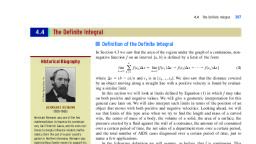
518, , Chapter 6 The Transcendental Functions, , 6.1, , The Natural Logarithmic Function, In this section we use the Fundamental Theorem of Calculus, Part 1, to define an important function: the natural logarithmic function. This approach affords a simple yet rigorous way of establishing all the properties of this function., Recall that the Fundamental Theorem of Calculus, Part 1, states that if f is a continuous function on an open interval I and if a is any number in I, then we can define, a differentiable function F by, x, , F(x) �, , 冮 f(t) dt, , x僆I, , a, , Now consider the function f defined by f(t) � 1>t on the interval (0, ⬁). (See Figure 1.), y, 2, , 1, y� t, , 1, , FIGURE 1, The function f(t) � 1>t, is continuous on (0, ⬁) ., , 0, , 1, , t, , 2, , Since f is continuous on (0, ⬁), the Fundamental Theorem of Calculus, Part 1, guarantees that we can define a differentiable function on (0, ⬁) as follows., , DEFINITION The Natural Logarithmic Function, The natural logarithmic function, denoted by ln, is the function defined by, ln x �, , 冮, , 1, , x, , 1, dt, t, , (1), , for all x � 0., , The expression ln x, read “ell-en of x,” is called the natural logarithm of x because, it has all the properties of logarithmic functions, as we shall see., Note, , You might recall that the power rule for integrals,, x, , 冮t, a, , n, , dt �, , t n�1 x, 1, ` �, (x n�1 � a n�1), n�1 a n�1, , is valid only for n � �1, since 1>(n � 1) would be undefined if n � �1. With the, definition of the integral for the function f(t) � 1>t � t �1, we now have a formula for, integrating f(t) � t n when n � �1. Thus,, , 冮, , 1, (x n�1 � a n�1), t dt � • n � 1, ln x � ln a, , a, , x, , n, , if n � �1, if n � �1, x � 0, and a � 0, , If x � 1, we can interpret ln x as the area of the region under the graph of y � 1>t, on the interval [1, x]. (See Figure 2.)
Page 3 :
6.1, y, , y, , 3, , 3, , 2, , 2, , 1, y� t, , 1, , 0, , FIGURE 2, ln x interpreted in terms of area, , The Natural Logarithmic Function, , 519, , 1, y� t, , 1, , 1, , x, , 2, , 0, , t, , 3, , x, , (a) If x > 1, ln x � y 1t dt, 1, , x, , 1, , 2, , 3, , t, , 1, (b) If 0 < x < 1, ln x � �y 1t dt, x, , For x � 1 we have, , 冮, , ln 1 �, , 1, , 1, , 1, dt � 0, t, , If 0 � x � 1, then, ln x �, , 冮, , x, , 1, , 1, dt � �, t, , 冮, , 1, , 1, dt � 0, t, , x, , so ln x can be interpreted as the negative of the area of the region under the graph of, y � 1>t on the interval [x, 1] (Figure 2b)., , The Derivative of ln x, Recall that the Fundamental Theorem of Calculus, Part 1, states that if f is continuous, on an open interval I and the function F is defined by, x, , F(x) �, , 冮 f(t) dt, , a僆I, , a, , then F¿(x) � f(x). Applying this theorem to the function f(t) � 1>t gives, d, d, ln x �, dx, dx, , 冮, , 1, , x, , 1, 1, dt �, x, t, , x�0, , (2), , Next, using the Chain Rule, we see that if u is a differentiable function of x, then, d, 1 du, ln u �, u dx, dx, , u�0, , (3), , Laws of Logarithms, The laws for differentiating the logarithmic function can be used to prove the following familiar laws of logarithms., , THEOREM 1 Laws of Logarithms, Let x and y be positive numbers and let r be a rational number. Then, a. ln 1 � 0, x, c. ln � ln x � ln y, y, , b. ln xy � ln x � ln y, d. ln x r � r ln x
Page 4 :
520, , Chapter 6 The Transcendental Functions, , PROOF, a. Law a was proved on page 519., b. Define the function F(x) � ln ax, where a is a positive constant. Then, using, Equation (3), we have, F¿(x) �, , d, 1 d, a, 1, (ln ax) �, (ax) �, �, ax dx, ax, x, dx, , But by Equation (2) we have, 1, d, ln x �, x, dx, Therefore, F(x) and ln x have the same derivative and, by Theorem 1 of Section, 4.1, must differ by a constant; that is,, F(x) � ln ax � ln x � C, Letting x � 1 in this equation and recalling that ln 1 � 0, we have, ln a � ln 1 � C � C, Therefore,, ln ax � ln x � ln a, Since a can be any positive number, we have shown that, ln xy � ln x � ln y, c. Using the result of part (b) with x � 1>y, we have, ln, , 1, 1, � ln y � lna ⴢ yb � ln 1 � 0, y, y, , so, ln, , 1, � �ln y, y, , Using the result of part (b) once again, we obtain, ln, , x, 1, 1, � lnax ⴢ b � ln x � ln � ln x � ln y, y, y, y, , as desired., d. Define the functions F and G by F(x) � ln x r and G(x) � r ln x, respectively., Then using Equation (3), we have, F¿(x) �, , 1, r, r�1, �, r ⴢ rx, x, x, , Next, using Equation (2), we find, G¿(x) �, , r, x, , Therefore, F and G must differ by a constant; that is,, ln x r � r ln x � C
Page 5 :
6.1, , The Natural Logarithmic Function, , 521, , Letting x � 1 in this equation gives, ln 1 � r ln 1 � C, or C � 0, so, ln x r � r ln x, as was to be shown., , EXAMPLE 1 Expand the expression:, a. ln, , x2 � 1, 1x, , b. ln, , x 3 cos2 px, 2x 2 � 1, , Solution, x2 � 1, x2 � 1, � ln 1>2 � ln(x 2 � 1) � ln x 1>2, Use Theorem 1c., 1x, x, 1, � ln(x 2 � 1) � ln x, Use Theorem 1d., 2, 3, 2, 3, 2, x (cos px), x cos px, b. ln, � ln 2, 2, (x � 1)1>2, 2x � 1, � ln x 3 � ln(cos px)2 � ln(x 2 � 1)1>2, Use Theorem 1b., 1, 2, � 3 ln x � 2 ln cos px � ln(x � 1), 2, a. ln, , EXAMPLE 2 Write ln x �, , 1, ln y as a single logarithm., 3, , Solution, ln x �, , 1, 3, ln y � ln x � ln y 1>3 � ln xy 1>3 � ln x1, y, 3, , The Graph of the Natural Logarithmic Function, To help us draw the graph of the natural logarithmic function, we first note that, f(x) � ln x has the following properties:, 1. The domain of f is (0, ⬁), by definition., 2. f is continuous on (0, ⬁), since it is differentiable there., 1, 3. f is increasing on (0, ⬁), since f ¿(x) � � 0 on (0, ⬁)., x, 1, 4. The graph of f is concave downward on (0, ⬁) since f ⬙(x) � � 2 � 0 on (0, ⬁)., x, Next, using the Trapezoidal Rule or Simpson’s Rule, we have, f(2) � ln 2 �, , 冮, , 1, , 2, , 1, dt ⬇ 0.693, t, , Then, using Theorem 1d, we obtain the following table of values., x, , 4, , 8, , f(x), , 1.386, , 2.079, , 1, 2, , 1, 4, , 1, 8, , �0.693 �1.386 �2.079
Page 6 :
522, , Chapter 6 The Transcendental Functions, , Using the properties of f(x) � ln x, the sample values just obtained, and the results, , y, y � ln x, , lim ln x � �⬁, , x→0�, , 1, , 0, , 1, , 2, , 3, , 4, , 5, , FIGURE 3, The graph of the natural logarithmic, function y � ln x, , x, , lim ln x � ⬁, , and, , x→⬁, , which we will establish at the end of this section, we sketch the graph of f(x) � ln x,, as shown in Figure 3., , The Derivatives of Logarithmic Functions, The rule for differentiating the natural logarithmic function was established earlier (see, Equations (2) and (3)). This rule holds in a more general setting, as stated in the following theorem., , THEOREM 2 Derivative of the Natural Logarithmic Function, Let u be a differentiable function of x. Then, a., , d, 1, ln 冟 x 冟 �, x, dx, , x�0, , b., , d, 1 du, ln 冟 u 冟 � ⴢ, u, dx, dx, , u�0, , PROOF, , a. If x � 0, then 冟 x 冟 � x, so by Equation (2) we have, d, d, 1, ln 冟 x 冟 �, ln x �, x, dx, dx, If x � 0, then 冟 x 冟 � �x � 0, so by Equation (3) we have, 1, d, d, 1 d, 1, ln 冟 x 冟 �, ln(�x) � �, (�x) � � (�1) �, x dx, x, x, dx, dx, b. This follows from the Chain Rule., , EXAMPLE 3 Find the derivative of, a. f(x) � ln(2x 2 � 1), , b. t(x) � x 2 ln 2x, , c. y � ln 冟 cos x 冟, , Solution, d, 1, d, 4x, ln(2x 2 � 1) � 2, (2x 2 � 1) � 2, dx, 2x � 1 dx, 2x � 1, d 2, d, d, b. t¿(x) �, (x ln 2x) � x 2, (ln 2x) � (ln 2x), (x 2), Use the Product Rule., dx, dx, dx, 1, � x 2 a b (2) � (ln 2x)(2x) � x(1 � 2 ln 2x), 2x, dy, d, 1 d, sin x, c., �, ln 冟 cos x 冟 �, (cos x) � �, � �tan x, cos x dx, cos x, dx, dx, a. f ¿(x) �, , If an expression contains a natural logarithm, it can be helpful to use the laws, of logarithms to simplify the expression before differentiating, as illustrated in Examples 4 and 5.
Page 7 :
6.1, , Historical Biography, , 523, , EXAMPLE 4 Find the derivative of f(x) � ln2x 2 � 1., Solution, , Science Source/Photo Researchers, Inc., , The Natural Logarithmic Function, , We first rewrite the given expression as, f(x) � ln(x 2 � 1)1>2 �, , 1, ln(x 2 � 1), 2, , Differentiating this function, we obtain, f ¿(x) �, JOHN NAPIER, , �, , (1550–1617), John Napier is famous for his invention of, the logarithm, which was described in two, of his publications: Mirifici logarithmorum, canonis descriptio (“A Description of the, Wonderful Canon of Logarithms”), published, in 1614, and Mirifici logarithmorum canonis, constructio (“The Construction of the Wonderful Canon of Logarithms”), published in, 1619. Born in 1550 at Merchiston Castle near, Edinburgh, Scotland, Napier came from a, line of influential noblemen. At 13 years of, age he entered the University of St., Andrews in Scotland, but he left after a, short time to study in Europe. It was during, this time that he developed a passion for, astronomy and mathematics, but he considered these pursuits a hobby, as theology, was his main interest. However, astronomy, so intrigued him that over the course of, two decades he developed logarithms to, work with the calculation of the extremely, large numbers that he needed to do, research in that area. Later, with Napier’s, consent, Henry Briggs made improvements, to Napier’s logarithms, such as using base, 10. Napier and Briggs’s important work was, essential to Johannes Kepler’s (page 889), study of planetary motion and therefore, ultimately to the work of Isaac Newton, (page 179). The work done by Napier and, Briggs also led to the standard form of the, logarithmic tables that remained in common use until the electronic age of calculators and computers., , d 1, 1 d, c ln(x 2 � 1)d � ⴢ, [ln(x 2 � 1)], dx 2, 2 dx, 1, 1, d 2, 1, 1, x, ⴢ 2, (x � 1) � ⴢ 2, (2x) � 2, 2 x � 1 dx, 2 x �1, x �1, , EXAMPLE 5 Find the rate of change of, f(x) � lnc, , x 2(2x 2 � 1)3, 25 � x 2, , d, , when x � 1., Solution The rate of change of f(x) for any value of x is given by f ¿(x). To find f ¿(x),, we first rewrite, f(x) � lnc, , x 2(2x 2 � 1)3, (5 � x ), , 2 1>2, , d � 2 ln x � 3 ln(2x 2 � 1) �, , 1, ln(5 � x 2), 2, , Then, we have, f ¿(x) �, �, , 3, d, d, 2, 1, � 2, (2x 2 � 1) �, (5 � x 2), 2, x, 2x � 1 dx, 2(5 � x ) dx, 12x, x, 2, � 2, �, x, 2x � 1, 5 � x2, , from which we see that the rate of change of f(x) at x � 1 is, f ¿(1) � 2 �, or, , 25, 4, , 12, 1, �, 3, 4, , units per unit change in x., , Logarithmic Differentiation, Having seen how the laws of logarithms can help to simplify the work involved in differentiating logarithmic expressions, we now look at a procedure that takes advantage, of these same laws to help us differentiate functions that at first blush do not necessarily involve logarithms. This method, called logarithmic differentiation, is especially, useful for differentiating functions involving products, quotients, and/or powers that, can be simplified by using logarithms.
Page 8 :
524, , Chapter 6 The Transcendental Functions, , EXAMPLE 6 Find the derivative of y �, Solution, getting, , (2x � 1)3, ., 13x � 1, , We begin by taking the natural logarithm on both sides of the equation,, , ln y � ln, , (2x � 1)3, (3x � 1)1>2, , or, ln y � 3 ln(2x � 1) �, , 1, ln(3x � 1), 2, , Use the laws of logarithms., , Next, we differentiate implicitly with respect to x, obtaining, 1, 3, 1, (y¿) �, (2) �, (3), y, 2x � 1, 2(3x � 1), �, , 6(2)(3x � 1) � 3(2x � 1), 6, 3, �, �, 2x � 1, 2(3x � 1), 2(2x � 1)(3x � 1), , �, , 15(2x � 1), 2(2x � 1)(3x � 1), , Multiplying both sides of this equation by y gives, y¿ �, �, �, , 15(2x � 1), ⴢy, 2(2x � 1)(3x � 1), 15(2x � 1), (2x � 1)3, ⴢ, 2(2x � 1)(3x � 1) 13x � 1, , Substitute for y., , 15(2x � 1)(2x � 1)2, 2(3x � 1)3>2, , Here is a summary of this procedure., Finding dy>dx by Logarithmic Differentiation, Suppose that we are given the equation y � f(x). To compute dy>dx:, 1. Take the logarithm of both sides of the equation, and use the laws of logarithms to simplify the resulting equation., 2. Differentiate implicitly with respect to x., 3. Solve the equation found in Step 2 for dy>dx., 4. Substitute for y., , Integration Involving Logarithmic Functions, By reversing the rule, 1 du, d, ln 冟 u 冟 �, u dx, dx, we obtain the following rule of integration.
Page 11 :
6.1, , Solution, , The Natural Logarithmic Function, , 527, , We have, S, � k(ln S � ln S0) � k ln S � k ln S0, S0, , R � k ln, So, , dR, d, �, (k ln S � k ln S0), dS, dS, , R, R � k ln S, S0, , 0, , S0, , FIGURE 4, The graph illustrating the WeberFechner Law, , k, S, , �, , S, , This says that the rate of change of the reaction with respect to the stimulus is, inversely proportional to the stimulus, with k as the constant of proportionality. Thus,, the rate of change of R decreases as S increases. This agrees with common experience—, one is more apt to detect the change in the volume or sound pressure level when it is, increased from 20 decibels (average whisper) to 22 decibels than when it is increased, from 70 decibels (busy street traffic) to 72 decibels. The graph of R � k ln(S>S0) is, shown in Figure 4., , EXAMPLE 13 Drug Concentration in the Bloodstream The concentration of a certain, drug (in mg/cc) in a patient’s bloodstream t hr after injection is, C(t) �, , 0.2t, t �1, 2, , Determine the average concentration of the drug in the patient’s bloodstream over the, first 4 hr after the drug is injected., Solution, , The average concentration of the drug over the time interval [0, 4] is given by, 1, 4�0, , A�, , 冮, , 0, , 4, , C(t) dt �, , 1, 4, , 冮, , 0, , 4, , 0.2t, t �1, 2, , dt, , To evaluate this definite integral, we make the substitution, u � t2 � 1, , so that, , du � 2t dt, , or, , t dt �, , du, 2, , Observe that when t � 0, u � 02 � 1 � 1, and when t � 4, u � 42 � 1 � 17, giving, u � 1 and u � 17 as the lower and upper limits of integration with respect to u, respectively. We have, A�, �, , 1, 20, , 冮, , 0, , 4, , t, t �1, , 1 1, a b, 20 2, , 2, , 冮, , 17, , 1, , dt, , 17, 1, 1, 1, du � c ln ud �, (ln 17 � ln 1), u, 40, 40, 1, , or approximately 0.071 mg/cc., We close this section by proving the following results., , THEOREM 5, a. lim ln x � ⬁, x→⬁, , b. lim� ln x � �⬁, x→0
Page 12 :
528, , Chapter 6 The Transcendental Functions, , PROOF, a. By Law (d) of logarithms (Theorem 1), we have ln 2n � n ln 2 for any positive, integer n. Since ln 2 � 0, as we demonstrated earlier, we see that ln 2n → ⬁ as, n → ⬁ . But ln x is an increasing function, so, lim ln x � ⬁, , x→⬁, , as was to be shown., b. Let t � 1>x. Then t → ⬁ as x → 0�. Therefore, using part (a), we have, 1, lim ln x � lim lna b � lim (�ln t) � �⬁, t→⬁, t, t→⬁, , x→0�, , 6.1, , CONCEPT QUESTIONS, , 1. Define the natural logarithmic function f(x) � ln x. What are, its domain and range?, 2. State the laws of logarithms., , 6.1, , EXERCISES, , In Exercises 1–4, given that ln 2 ⬇ 0.6931, ln 3 ⬇ 1.0986, and, ln 5 ⬇ 1.6094, use the laws of logarithms to approximate each, expression., 1. a. ln 6, , 3, b. ln, 2, , 20, 2. a. ln, 13, , 15 1>3, b. lna b, 2, , 3. a. ln 30, , b. ln 7.5, , 4. a. ln, , 1, 125, , b. ln, , 5, 9, , In Exercises 5–10, use the laws of logarithms to expand the, expression., 5. ln, 7. ln, , 213, 5, , 6. ln, , x 1>3y 2>3, , z 1>2, x � 1 1>3, b, 9. lna, x�1, , xy, z, , 8. ln 1 x 22x 2 � 1 2, 10. lnC 1x 冟 cos x 冟(x � 1)�1>3 D, , In Exercises 11–14, use the laws of logarithms to write the, expression as the logarithm of a single quantity., 11. ln 4 � ln 6 � ln 12, 13. 3 ln 2 �, , 3. Let f(x) � ln x 2 and t(x) � 2 ln x. Are f and t identical?, Explain., 4. Is the function f(x) � ln 1 x � 21 � x 2 2 odd, even, or neither odd nor even? Explain., , 12. ln(x 2 � 1) � 2 ln(x � 1), , 1, ln(x � 1), 2, , 1, 14. [2 ln(x � 1) � ln x � ln(x � 1)], 2, , In Exercises 15–20, use the graph of y � ln x as an aid to sketch, the graph of the function., 15. f(x) � 2 ln x, , 16. t(x) � �ln x, , 17. y � 1 � ln x, , 18. f(x) � ln 2x, , 19. t(x) � ln(x � 1), , 20. h(x) � ln 冟 x 冟, , In Exercises 21–24, find the domain of the function., 21. f(x) � ln(2x � 1), , 22. t(x) � ln(�x), , 23. t(x) � ln(cos x), , 24. h(x) � lna, , x�1, b, x�1, , 25. a. Plot the graphs of f(x) � ln x � ln(x � 1) and, t(x) � ln x(x � 1) using the same viewing window., b. For what values of x is f � t? Prove your assertion., 26. a. For what values of x is f � t if f(x) � ln 1x>(x � 1) and, t(x) � 12 [ln x � ln(x � 1)]?, b. Verify the result of part (a) graphically by plotting the, graphs of f and t., In Exercises 27–48, differentiate the function., 27. f(x) � ln(2x � 3), , 28. t(x) � ln(x 2 � 4)2, , 29. h(x) � ln 1x, , 30. y � 1ln x, , 31. t(u) � ln, , u, u�1, , 33. y � x(ln x)2, 35. t(x) �, , V Videos for selected exercises are available online at www.academic.cengage.com/login., , ln x, x�1, , 32. t(t) � t ln 2t, 34. f(x) � ln 1 x � 2x 2 � 1 2, 36. y � lna, , x � 1 2>3, b, x�1
Page 13 :
6.1, , 38. h(t) �, , 37. f(x) � ln(ln x), , ln t, ln 2t, , 40. f(x) � ln[x ln(x � 2)], , 41. t(x) � sin(ln x), , 42. h(t) � t sin(ln 2t), , 43. f(x) � x 2 ln cos x, , 44. t(u) � ln 冟 tan 3u 冟, , 45. h(u) � ln 冟 sec u 冟, , 46. f(x) � sec[ln(2x � 3)], , sin t � 1, `, cos t � 2, , 48. t(x) � ln, , 71., 73., , 51. ln, , 75., , x cos x, , 冮, , 1, , x2, 3x 3 � 1, , 冮x, , 冮, , 3, , 78., , 冮, , 11 � ln x, dx, x, , 1, , (x � 1), 1, dx, x ln x, 1>3, , dx, , 76., , 1, , x2 � x � 3, dx, x, ln x, dx, x, , 50. ln xy � y � 5, , 80., , 冮 4 � tan 3x dx, , 52. ln(x � y) � cos y � x 2 � 0, , 81., , 冮 (sec u � cos u) du, , 82., , 冮 1 � sin x dx, , 83., , 冮 2 � x ln x dx, , 84., , 冮, , x 2y⬙ � 3xy¿ � 4y � 0, x y⬙ � xy¿ � 5y � 0, 2, , 56. Find an equation of the tangent line to the curve, y � ln(x 2 � y 2) � 0 at (1, 0)., , cos x, , 1 � ln x, , sec2 3x, sin 2x, , 2, , (ln x) 11 � ln x, dx, x, , 85. Find the area of the region bounded by the graphs of, 1, x, y� 2, , y � � x 2, and x � 1., 2, x �1, 86. The region under the graph of y � 1>(x 2 � 1) on the interval [0, 2] is revolved about the y-axis. Find the volume of, the resulting solid., 87. Find the length of the graph of, , In Exercises 57 and 58, find the absolute extrema of the function, on the indicated interval., ln x � 1, ;, x, , 冮, , 3, , 74., , 1, 2>3, , 1, , 冮 1 � sin x dx, , 55. Find an equation of the tangent line to the graph of, y � x ln x at (1, 0)., , 58. f(x) �, , dx, , 冮 2x � 3 dx, , 79., , 54. y � x cos(2 ln x) � 3x sin(2 ln x);, , 57. f(x) � x ln x � x;, , 72., , 冮, , In Exercises 53 and 54, show that the function y � f(x) is a, solution of the given differential equation., 53. y � 2x 2 � 3x 2 ln x;, , 2, , 77., , B (2x � 1), , 3, , 2, , x, � x � y2 � 0, y, , 冮 3x dx, 0, , In Exercises 49–52, use implicit differentiation to find dy>dx., 49. ln y � x ln x � �1, , 529, , In Exercises 71–84, find or evaluate the integral., , 39. f(x) � ln(x ln x), , 47. t(t) � ln `, , The Natural Logarithmic Function, , C 12, 2D, , y�, , 1, Cx2x 2 � 1 � ln 1 x � 2x 2 � 1 2 D, 2, , on the interval [1, 3]., , C 12, 3D, , 88. Find the length of the graph of y � ln cos x on the interval, C0, p4 D ., , In Exercises 59–62, use the guidelines of Section 3.6 to sketch, the graph of the function., , 89. Find the centroid of the region bounded by the graphs of, y � 1>x, y � 0, x � 1, and x � 2., , 59. f(x) � x � ln x, , 90. Show that, , 60. f(x) � x ln x � x, , 91. Find, �p2 � x � p2, , In Exercises 63 and 64, use Newton’s method to find the roots of, the equation correct to five decimal places., 63. x ln x � 1 � 0, , 64. ln x � x � 3 � 0, , In Exercises 65–68, use logarithmic differentiation to find the, derivative of the function., 65. y � (2x � 1)2(3x 2 � 4)3, 67. y �, , 3, , x�1, , Bx � 1, 2, , 69. Find y⬙ if y � x x., , x 2 ln, , �1>2, , 61. f(x) � ln(x 2 � 1), 62. f(x) � ln(cos x),, , 冮, , 1>2, , 66. y �, 68. y �, , x 2 12x � 4, (x � 1)2, sin2 x, x 11 � tan x, 2, , x, , 70. Find y¿ if y � x x ., , dy, if y �, dx, , 92. Let y �, , 冮, , x2, , 2>x, , 冮, , 1�x, dx � 0., 1�x, , x2, , ln t dt, where x � 0., , x, , dt, , where x � 2., t, , a. Find dy>dx by finding the integral and then differentiating the result., b. Find dy>dx using the Fundamental Theorem of Calculus,, Part 1., 93. A sports sedan traveling along a straight road attains a, velocity of √(t) � 1056t>(t 2 � 36) ft/sec after t sec. How, far does it travel in the first 20 sec?, 94. Flight of a Rocket A rocket having mass M kg and carrying, fuel of mass m kg takes off vertically from the earth’s surface. The fuel is burned at the constant rate of a kg/sec, and, the gas is expelled at a constant velocity of b m/sec relative
Page 14 :
530, , Chapter 6 The Transcendental Functions, to the rocket, where a � 0 and b � 0. If the external force, acting on the rocket is a constant gravitational field, then the, height of the rocket t seconds after liftoff is, x � bt �, , M � m � at, 1, b, (M � m � at)lna, b � tt 2, a, M�m, 2, 0 t, , f(x) � 7.2956 ln(0.0645012x 0.95 � 1), m, a, , a. Find expressions for the velocity and acceleration of the, rocket at any time t after liftoff., b. What are the velocity and acceleration of the rocket at, burnout (that is, when t � m>a)., 95. Distance Traveled by a Motorboat The distance x (in feet) traveled by a motorboat moving in a straight line t sec after the, engine of the moving boat has been cut off is given by, x�, , 98. Strain on Vertebrae The strain (percentage of compression), on the lumbar vertebral disks in an adult human as a function of the load x (in kilograms) is given by, , 1, ln(√0kt � 1), k, , where k is a constant and √0 is the speed of the boat at t � 0., a. Find expressions for the velocity and acceleration of the, boat at any time t after the engine has been cut off., b. Show that the acceleration of the boat is in the direction, opposite to that of its velocity and is directly proportional to the square of its velocity., c. Use the results of part (a) to show that the velocity of the, boat after traveling a distance of x ft is given by, , What is the rate of change of the strain with respect to the, load when the load is 100 kg? When the load is 500 kg?, Source: Benedek and Villars, Physics with Illustrative Examples, from Medicine and Biology., , 99. Predator-Prey Model The relationship between the number of, rabbits y(t) and the number of foxes x(t) at any time t is, given by, �C ln y � Dy � A ln x � Bx � E, where A, B, C, D, and E are constants. This relationship, is based on a model by Lotka (1880–1949) and Volterra, (1860–1940) for analyzing the ecological balance between, two species of animals, one of which is a prey species and, the other of which is a predator species. Use implicit differentiation to find the relationship between the rate of, change of the rabbit population in terms of the rate of, change of the fox population., 100. Work Done by an Expanding Gas In Example 6 in Section 5.5, we showed that the work done by an expanding gas against, a piston as its volume expands from V0 to V1 is given by, , √ � √0e�kx, , W�, , 96. Growth of a Tumor The rate at which a tumor grows with, respect to time is given by, R � Ax ln, , B, x, , for 0 � x � B, where A and B are positive constants and x, is the radius of the tumor., a. Plot the graph of R for the case A � B � 10., b. Use the graph of part (a) to estimate the radius of the, tumor when the tumor is growing most rapidly with, respect to time., 97. Annuities At the time of retirement, Christine expects to have, a sum of $500,000 in her retirement account. Her accountant, pointed out to her that if she made withdrawals in monthly, installments amounting to x dollars per year (x � 25,000),, assuming that the account earns interest at the rate of 5% per, year compounded continuously, then the time required to, deplete her savings would be T years, where, T � f(x) � 20 lna, , x, b, x � 25,000, , x � 25,000, , a. Plot the graph of f, using the viewing window, [25,000, 50,000] � [0, 100]., b. How much should Christine plan to withdraw from her, retirement account each year if she wants it to last for, 25 years?, c. Evaluate lim x→25,000� f(x). Is the result expected? Explain., , 冮, , V1, , p dV, , V0, , where p is the pressure of the gas. If the pressure and volume of a gas are related by the equation pV � k, where k, is a positive constant, show that W � k ln(V1>V0)., , gas, , As the gas expands, work is done by, the expanding gas against the piston., 101. Work Done by an Expanding Gas Refer to Exercise 100. At, high pressure, the relationship between the volume V and, pressure P of gases is approximated by the van der Waals, equation:, aP �, , an 2, V2, , b (V � nb) � nRT, , where R is the gas constant, n is the number of moles, and, a and b are constants having different values for different, gases. (In the special case in which a � b � 0, we have, the ideal gas equation.) Calculate the work done by a van, der Waals gas when it undergoes isothermal expansion, (T � constant) from a volume of V0 to a volume of V1., Reconcile your result with that of Exercise 100 when, a � b � 0 (that is, when expansion occurs under normal, pressure).
Page 15 :
6.1, 102. Force Exerted by an Electric Charge An electric charge Q is, distributed uniformly along a line of length 2a, lying along, the y-axis, as shown in the figure. A point charge q lies on, the x-axis, at a distance x from the origin. It can be shown, that the magnitude of the total force F that Q exerts on q, (in the direction of the x-axis) is F � �q dV>dx, where, V(x) �, , 2a 2 � x 2 � a, 1 Q, ln, 4pe0 2a 2a 2 � x 2 � a, , e0, a constant, , 531, , 105. Rate of a Catalytic Chemical Reaction A catalyst is a substance, that either accelerates a chemical reaction or is necessary, for the reaction to occur. Suppose that an enzyme E (a, catalyst) combines with a substrate S (a reacting chemical), to form an intermediate product X, which then produces a, product P and releases the enzyme. If initially there are x 0, moles per liter of S and there is no P, then on the basis of, the theory of Michaelis and Menten, the concentration of, P, p(t), after t hours is given by the equation, , Show that, , Vt � p � k lna1 �, , qQ, 1, F�, 2, 4pe0 x2x � a 2, , p, b, x0, , where the constant V is the maximum possible speed of, the reaction and the constant k is called the Michaelis, constant for the reaction. Find the rate of change of the, formation of the product P in this reaction., , y, a, , The Natural Logarithmic Function, , 106. Heights of Children For children between the ages of 5 and, 13 years, the Ehrenberg equation, , Q, q, , 0, , F, , x, , ln W � ln 2.4 � 1.84h, , x, , gives the relationship between the weight W (in kilograms), and the height h (in meters) of a child. Use differentials to, estimate the change in the weight of a child who grows, from 1 m to 1.1 m., , �a, , A line of charge with length 2a and total charge Q exerts, an electrostatic force on the point charge q., 103. Average Temperature A homogenous hollow metallic ball of, inner radius r1 and outer radius r2 is in thermal equilibrium. The temperature T at a distance r from the center of, the ball is given by, r1r2(T2 � T1) 1, 1, T � T1 �, a � b, r, r1, (r1 � r2), , r1, , r, , r2, , where T1 is the temperature on the inner surface and T2 is, the temperature on the outer surface. Find the average temperature of the ball in a radial direction between r � r1, and r � r2., 104. Motion of a Submersible A submersible moving in a straight, line through water is subjected to a resistance R that is proportional to its velocity. Suppose that the submersible travels with its engine shut off. Then the time it takes for the, submersible to slow down from a velocity of √1 to a velocity of √2 is, T��, , 冮, , √2, , √1, , m, d√, k√, , where m is the mass of the submersible and k is a constant., Find the time it takes the submersible to slow down from a, velocity of 16 ft/sec to 8 ft/sec if its mass is 1250 slugs, and k � 20 (slug/sec)., , 107. Use Simpson’s Rule with n � 8 to find an approximation, of 兰12 ln x 2 dx. Give an upper bound for the error incurred, in this approximation., Hint: Use Equation (5) of Section 4.6., , 108. Plot the graph of y � cos(p ln x) on the interval [1, 2]., Then, using a computer or a calculator, find the approximate length of the graph., In Exercises 109–116, determine whether the statement is true or, false. If it is true, explain why it is true. If it is false, give an, example to show why it is false., 109. ln a � ln b � ln(a � b) for all positive numbers, a � b � 0., 110. (ln x)3 � 3 ln x for all x in (0, ⬁)., 111. The domain of f(x) � ln 冟 x 冟 is (�⬁, 0) 傼 (0, ⬁)., 112. If f(x) � ln x and 0 � a � b, then f(a) � f(b) ., 113. The function f(x) � 1>(ln x) is continuous on (1, ⬁) ., 114. If f(x) � ln 5, then f ¿(x) � 15 ., 3, , 115., , 冮 x � 2 � �冮, 1, , 116., , 1, , dx, , 3, , 2, , dx, x�2, , 2, dx, � ln 冟 x 冟 ` � ln 冟 2 冟 � ln 冟 �2 冟 � ln 2 � ln 2 � 0, �2, �2 x, , 冮
Page 16 :
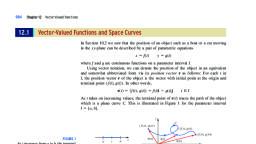
532, , Chapter 6 The Transcendental Functions, , 6.2, , Inverse Functions, The Inverse of a Function, Consider the position function, s � f(t) � 4t 2, , 0, , t, , 30, , (1), , giving the position of a maglev at any time t in its domain [0, 30]. The graph of f is, shown in Figure 1. Equation (1) enables us to compute algebraically the position of, the maglev at any given time t. Geometrically, we can find the position of the maglev, at any given time t by following the path indicated in Figure 1, which associates the, given time t with the desired position f(t)., , s (ft), 3600, 3000, f(t), , s � 4t 2, , 2000, Range of f, 1000, 0, , 10, 20, Domain of f, , t, , 30, , t (sec), , FIGURE 1, Each t in the domain of f is associated with the (unique) position s � f(t) of the maglev., , Now consider the reverse problem: Knowing the position function of the maglev,, can we find some way of obtaining the time it takes for the maglev to reach a given, position? Geometrically, this problem is easily solved: Locate the point on the, s-axis corresponding to the given position. Follow the path considered earlier but, traced in the opposite direction. This path associates the given position s with the, desired time t., Algebraically, we can obtain a formula for the time t it takes for the maglev to get, to the position s by solving Equation (1) for t in terms of s. Thus,, t�, , 1, 1s, 2, , (we reject the negative root, since t lies in [0, 30]). Observe that the function t defined by, t � t(s) �, , 1, 1s, 2, , has domain [0, 3600] (the range of f ) and range [0, 30] (the domain of f ). The graph, of t is shown in Figure 2.
Page 17 :
6.2, , Inverse Functions, , 533, , t (sec), 30, g(s), , t � g(s), , 20, Range of g, 10, , FIGURE 2, Each s in the domain of t is associated, with the (unique) time t � t(s)., , s, 1000 2000 3000, Domain of g, , 0, , s (ft), , The functions f and t have the following properties:, 1. The domain of t is the range of f and vice versa., 2. They satisfy the relationships, (t ⴰ f )(t) � t[f(t)] �, , 1, 1, 1f(t) � 24t 2 � t, 2, 2, , and, 2, 1, ( f ⴰ t)(t) � f [t(t)] � 4[t(t)]2 � 4a 1tb � t, 2, , In other words, one undoes what the other does. This is to be expected because f maps, t onto s � f(t) and t maps s � f(t) back onto t., The functions f and t are said to be inverses of each other. More generally, we have, the following definition., , DEFINITION Inverse Functions, A function t is the inverse of the function f if, f [t(x)] � x for every x in the domain of t, and, t[f(x)] � x for every x in the domain of f, Equivalently, t is the inverse of f if the following condition is satisfied:, y � f(x), , if and only if, , x � t(y), , for every x in the domain of f and for every y in its range., , Note The inverse of f is normally denoted by f �1 (read “f inverse”), and we will use, this notation throughout the text., , !, , Do not confuse f �1(x) with [ f(x)]�1 �, , 1, ., f(x)
Page 18 :
534, , Chapter 6 The Transcendental Functions, , EXAMPLE 1 Show that the functions f(x) � x 1>3 and t(x) � x 3 are inverses of each, other., Solution First, observe that the domain and range of both f and t are (�⬁, ⬁). Therefore, both the composite functions f ⴰ t and t ⴰ f are defined. Next, we compute, ( f ⴰ t)(x) � f [t(x)] � [t(x)]1>3 � (x 3)1>3 � x, and, y�, , y, , (t ⴰ f )(x) � t[f(x)] � [ f(x)]3 � (x 1>3)3 � x, , x3, , y�x, , Since f [t(x)] � x for all x in (�⬁, ⬁), and t[f(x)] � x for all x in (�⬁, ⬁) , we, conclude that f and t are inverses of each other. In short, f �1(x) � x 3., , 2, y � x1/3, 1, , Interpreting Our Results, �2, , 0, , �1, , 1, , x, , 2, , We can view f as a cube root extracting machine and t as a “cubing” machine. In this, light, it is easy to see that one function does undo what the other does. So f and t are, indeed inverses of each other., , �1, �2, , FIGURE 3, The functions y � x 1>3 and y � x 3, are inverses of each other., y, , y � f �1(x), , The Graphs of Inverse Functions, The graphs of f(x) � x 1>3 and f �1(x) � x 3 are shown in Figure 3. They seem to suggest that the graphs of inverse functions are mirror images of each other with respect, to the line y � x. This is true in general, as we will now show., Suppose that (a, b) is any point on the graph of a function f. (See Figure 4.) Then, b � f(a), and we have, , y�x, , f �1(b) � f �1[ f(a)] � a, , (b, a), , a, , y � f(x), b, , (a, b), 0 b, , x, , a, , FIGURE 4, The graph of f �1, , This shows that (b, a) is on the graph of f �1 (Figure 4). Similarly, we can show that, if (b, a) lies on the graph of f �1, then (a, b) must be on the graph of f. But the point, (b, a), as you can see in Figure 4, is the reflection of the point (a, b) with respect to, the line y � x. We have proved the following., , The Graphs of Inverse Functions, The graph of f �1 is the reflection of the graph of f with respect to the line y � x, and vice versa., , y � f �1(x), , y, , y�x, , 3, , EXAMPLE 2 Sketch the graph of f(x) � 1x � 1. Then reflect the graph of f with, respect to the line y � x to obtain the graph of f �1., , 2, y � √x � 1, , 1, , 0, , 1, , 2, , 3, , FIGURE 5, The graph of f �1 is obtained by, reflecting the graph of f with, respect to the line y � x., , 4, , Solution, x, , The graphs of both f and f �1 are sketched in Figure 5., , Which Functions Have Inverses, Does every function have an inverse? Consider, for example, the function f defined by, y � x 2 with domain (�⬁, ⬁) and range [0, ⬁) . From the graph of f shown in Figure 6,, you can see that each value of y in the range of [0, ⬁) of f is associated with exactly, two numbers x � 1y in the domain (�⬁, ⬁) of f (except for y � 0). This implies
Page 19 :
6.2, y, y � x2, y, , 0, , � √y, , x, , √y, , FIGURE 6, Each value of y is associated with two, values of x., y, y � x2, , Inverse Functions, , 535, , that f does not have an inverse, since the uniqueness requirement of a function cannot, be satisfied in this case. Observe that any horizontal line y � c, where c � 0, intersects the graph of f at more than one point., Next, consider the function t defined by the same rule as that of f, namely, y � x 2,, but with domain restricted to [0, ⬁). From the graph of t shown in Figure 7, you can, see that each value of y in the range [0, ⬁) of t is mapped onto exactly one number, x � 1y in the domain [0, ⬁) of t. Thus, in this case we can define the inverse function of t, from the range [0, ⬁) of t, onto the domain [0, ⬁) of t. To find the rule for, t�1, we solve the equation y � x 2 for x in terms of y. Thus, x � 1y, since x 0, so, t�1(y) � 1y, or, since y is a dummy variable, we can write t�1(x) � 1x. Also, observe, that every horizontal line intersects the graph of t at no more than one point., Our analysis of the functions f and t reveals the following important difference, between the two functions that enables t to have an inverse but not f. Observe that f, takes on the same value twice; that is, there are two values of x that are mapped onto, each value of y (except y � 0). On the other hand, t never takes on the same value, more than once; that is, any two values of x have different images. The function t is, said to be one-to-one., , y, , DEFINITION One-to-One Function, A function f with domain D is one-to-one if no two numbers in D have the same, image; that is,, 0, , x, , √y, , f(x 1) � f(x 2), , FIGURE 7, Each value of y is associated, with exactly one value of x., , whenever, , x1 � x2, , Geometrically, a function is one-to-one if every horizontal line intersects its graph, at no more than one point. This is called the horizontal line test., We have the following important theorem concerning the existence of an inverse, function., , THEOREM 1 The Existence of an Inverse Function, A function has an inverse if and only if it is one-to-one., , You will be asked to prove this theorem in Exercise 59., y, , EXAMPLE 3 Determine whether the function has an inverse., 3, , y�, , x3, , � 3x � 1, y�1, , � √3, , 0, �1, , √3, , FIGURE 8, f is not one-to-one because it fails the, horizontal line test., , x, , a. f(x) � x 1>3, , b. f(x) � x 3 � 3x � 1, , Solution, a. Refer to Figure 3, page 534. Using the horizontal line test, we see that f is oneto-one on (�⬁, ⬁). Therefore, f has an inverse on (�⬁, ⬁)., b. The graph of f is shown in Figure 8. Observe that the horizontal line y � 1 intersects the graph of f at three points, so f does not pass the horizontal line test., Therefore, f is not one-to-one. In fact, the three points x � � 13, 0, and 13, are mapped onto the point 1. Therefore, by Theorem 1, f does not have an, inverse.
Page 20 :
536, , Chapter 6 The Transcendental Functions, , Finding the Inverse of a Function, Before looking at the next example, let’s summarize the steps for finding the inverse, of a function, assuming that it exists., , Guidelines for Finding the Inverse of a Function, 1. Write y � f(x)., 2. Solve this equation for x in terms of y (if possible)., 3. Interchange x and y to obtain y � f �1(x)., , EXAMPLE 4 Find the inverse of the function defined by f(x) �, , Solution The graph of f shown in Figure 9 shows that f is one-to-one and so f �1, exists. To find the rule for this inverse, write, , y � f �1(x) � 3x �2 1, 2x, 2, , y, , 1, ., 12x � 3, , y�x, 3, , y�, , 2, , 1, 12x � 3, , and then solve the equation for x:, 1, y � f(x) �, √2x � 3, , 1, , 0, , 1, , 2, , 3, , y2 �, , x, , 2x � 3 �, , FIGURE 9, The graphs of f and f �1. Notice that, they are reflections of each other with, respect to the line y � x., , 2x �, , 1, 2x � 3, , Square both sides., , 1, , Take reciprocals., , y2, 1, y2, , �3�, , 3y 2 � 1, y2, , and, x�, , 3y 2 � 1, 2y 2, , Finally, interchanging x and y, we obtain, y�, , 3x 2 � 1, 2x 2, , giving the rule for f �1 as, f �1(x) �, , 3x 2 � 1, 2x 2, , The graphs of both f and f �1 are shown in Figure 9., , Continuity and Differentiability of Inverse Functions, Because of the reflective property of inverse functions, we might expect that f and f �1, have similar properties. More specifically, we have the following theorem whose proof, is given in Appendix B.
Page 21 :
6.2, , Inverse Functions, , 537, , THEOREM 2 Continuity and Differentiability of Inverse Functions, Let f be one-to-one, so that it has an inverse f �1., 1. If f is continuous on its domain, then f �1 is continuous on its domain., 2. If f is differentiable at c and f ¿(c) � 0, then f �1 is differentiable at f(c)., The next theorem shows us how to compute the derivative of an inverse function., , THEOREM 3 The Derivative of an Inverse Function, Let f be differentiable on its domain and have an inverse function t � f �1. Then, the derivative of t is given by, t¿(x) �, , 1, f ¿[t(x)], , (2), , provided that f ¿[t(x)] � 0., , PROOF By Theorem 2, t is differentiable. Next, using the definition of the inverse, function, we have, x � f [t(x)], Differentiating both sides of this equation with respect to x using the Chain Rule, we, find, 1�, , d, f [t(x)] � f ¿[t(x)]t¿(x), dx, , from which we see that, t¿(x) �, , 1, f ¿[t(x)], , Note If we write y � f �1(x) � t(x), then x � f(y), and we can write Equation (2) in, the form, dy, 1, �, dx, dx, dy, , EXAMPLE 5 Let f(x) � x 2 for x in [0, ⬁)., a. Show that the point (2, 4) lies on the graph of f., b. Find t¿(4), where t is the inverse of f., Solution, a. Since f(2) � 4, we conclude that the point (2, 4) does lie on the graph of f., b. Since f ¿(x) � 2x, Equation (2) gives, t¿(4) �, , 1, 1, 1, 1, 1, �, �, `, �, �, f ¿[t(4)], f ¿(2), 2x x�2 2(2), 4, , (3)
Page 22 :
538, , Chapter 6 The Transcendental Functions, , 6.2, , CONCEPT QUESTIONS, 3. Suppose that f is a one-to-one function defined by y � f(x)., a. Describe how to find the rule for f �1. Give an example., b. Describe the relationship between the graph of f and that, of f �1., 4. Suppose that f is differentiable and has an inverse t. How do, you find t¿?, , 1. a. What is a one-to-one function? Give an example., b. Explain how the horizontal line test is used to determine, whether a curve in the plane is the graph of a one-to-one, function. Illustrate with a figure., 2. Suppose that f is a one-to-one function with domain [a, b], and range [c, d]., a. How is f �1 defined?, b. What are the domain and range of f �1? Illustrate with a, figure., , 6.2, , EXERCISES, , In Exercises 1–6, show that f and t are inverses of each other by, verifying that f [t(x)] � x and t[ f(x)] � x., 1, 1. f(x) � x 3;, 3, 1, 2. f(x) � ;, x, , t(x) �, , y, , 0);, , x�3, 2, t(x) � � 1x � 1, , 13. f(x) � 4x � 3, , 5. f(x) � 4(x � 1) , where x �1;, 1, t(x) � (x 3>2 � 8), where x 0, 8, t(x) �, , 14. f(x) � �x 2 � 2x � 3, 15. f(x) � 11 � x, 16. f(x) � x 3 � x � 2, , x�1, x�1, , 17. f(x) � �x 4 � 16, 18. f(x) � 冟 x � 1 冟 � 冟 x 冟, , In Exercises 7–12, you are given the graph of a function f., Determine whether f is one-to-one., 8., , y, , 0, , In Exercises 13–18, determine whether the function is one-toone., , 2>3, , 1�x, ;, 1�x, , x, , 0, , 1, x, , t(x) �, , 4. f(x) � x 2 � 1 (x, , 7., , 12., , y, , 3, t(x) � 1, 3x, , 3. f(x) � 2x � 3;, , 6. f(x) �, , 11., , 19. Suppose that f is a one-to-one function such that f(2) � 5., Find f �1(5) ., , y, , 20. Suppose that f is a one-to-one function such that f(3) � 7., Find f [ f �1(7)]., In Exercises 21–26, find f �1(a) for the function f and the real, number a., , 0, , x, , x, , 0, , 21. f(x) � x 3 � x � 1; a � �1, 22. f(x) � 2x 5 � 3x 3 � 2; a � 2, , 9., , 10., , y, , y, , 23. f(x) �, , 3, x � sin x; �p2 � x � p2 ; a � 1, p, , 24. f(x) � 2 � tana, , px, b , �1 � x � 1; a � 2, 2, , 25. f(x) � cot(2x) , 0 � x � p2 ; a � 0, 0, , x, , 0, , x, , 26. f(x) �, , V Videos for selected exercises are available online at www.academic.cengage.com/login., , 1, 3, � x� ,, 2 B, 4, , x, , 3, 4;, , a�1, , x
Page 23 :
6.2, 27. The graph of f is given. Sketch the graph of f �1 on the same, set of axes., y, , y � f (x), , Inverse Functions, , 539, , 40. a. Show that f(x) � �x 2 � x � 1 on C 12, ⬁ 2 and, t(x) � 12 � 254 � x on 1 �⬁, 54 2 are inverses of each, other., b. Solve the equation �x 2 � x � 1 � 12 � 254 � x., Hint: Use the result of part (a)., , 1, , �1, , 1, , x, , �1, , 28. The graph of the inverse of a function f, f �1, is given., Sketch the graph of f on the same set of axes., y, , y � f �1(x), , 1, , 41. Temperature Conversion The formula F � f(C) � 95 C � 32,, where C �273.15, gives the temperature F (in degrees), on the Fahrenheit scale as a function of the temperature C, (in degrees) on the Celsius scale., a. Find a formula for f �1, and interpret your result., b. What is the domain of f �1?, 42. Motion of a Hot Air Balloon A hot air balloon rises vertically, from the ground so that its height after t sec is, h � 12 t 2 � 12 t, where h is measured in feet and 0 t 60., a. Find the inverse of the function f(t) � 12 t 2 � 12 t and, explain what it represents., b. Use the result of part (a) to find the time when the, balloon is between an altitude of 120 ft and 210 ft., 43. Aging Population The population of Americans age 55 and, over as a percent of the total population is approximated, by the function, , 0, , 1, , x, , f(t) � 10.72(0.9t � 10)0.3, , In Exercises 29–34, find the inverse of f. Then sketch the graphs, of f and f �1 on the same set of axes., 30. f(x) � x 2,, , 29. f(x) � 3x � 2, 31. f(x) � x � 1, , x, , 0, , 32. f(x) � 21x � 3, , 3, , 33. f(x) � 29 � x ,, 2, , x, , 0, , In Exercises 35–38, find the inverse of f. Then use a graphing, utility to plot the graphs of f and f �1 using the same viewing, window., 3, 35. f(x) � 1, x�1, , 37. f(x) �, 38. f(x) �, , x, , , �12, , x, 2x 2 � 1, , ,, , �1, , 25, , where t is measured in years and t � 0 corresponds to the, year 2000., a. Find the rule for f �1., b. Evaluate f �1(25), and interpret your result., Source: U.S. Census Bureau., , 1, 2, , x, x, , m0, , m � f(√) �, B, , 1�, , √2, c2, , where m 0 is the rest mass (the mass at zero speed) and, c � 2.9979 � 108 m/sec is the speed of light in a vacuum., a. Find f �1, and interpret your result., b. What is the speed of a particle when its relativistic mass, is four times its rest mass?, , 1, x, , x2 � 1, , t, , 44. Special Theory of Relativity Refer to Example 2, page 293., According to the special theory of relativity, the relativistic, mass of a particle moving with speed √ is, , 34. f(x) � x 3>5 � 1, , 36. f(x) � 1 �, , 0, , 1, , 39. Let, 2x � 1, if x � 1, 1x, if 1 x � 4, f(x) � μ, 1 2, x � 6 if x 4, 2, Find f �1(x), and state its domain., , 45. Suppose that f(x) � x 2 for x in [0, ⬁), and let t be the, inverse of f., a. Compute t¿(x) using Equation (2)., b. Find t¿(x) by first computing t(x)., 46. Let f(x) � x 1>3, and let t be the inverse of f., a. Find t¿(x) using Equation (2)., b. Find t¿(x) by first computing t(x).
Page 24 :
540, , Chapter 6 The Transcendental Functions, , In Exercises 47–54, let t denote the inverse of the function f., (a) Show that the point (a, b) lies on the graph of f. (b) Find, t¿(b)., 47. f(x) � 2x � 1;, , 48. f(x) � x 3 � x � 2;, , (2, 5), , 49. f(x) � x � 2x � x � 1;, 5, , 50. f(x) �, , x�1, ;, 2x � 1, 3, , 52. f(x) � 2 � 1x � 1;, 53. f(x) �, , 1, 1�x, 1, , 54. f(x) �, , 2, , 51. f(x) � (x 3 � 1)3;, , (1, 2), , (1, 4), , (0, �1), , 3, , (1, 8), , (7, 0), , , where x, , 0;, , , where x, , ( f �1)¿(a) �, , 56. Suppose that t is the inverse of a differentiable function, f and H � t ⴰ t. If f(4) � 3, t(4) � 5, f ¿(4) � 12 , and, f ¿(5) � 2, find H¿(3) ., , 冮, , 2, , x, , dt, 21 � t 3, , , where x � �1, what is ( f �1)¿(0) ?, , 58. Prove that if f has an inverse, then ( f �1)�1 � f., 59. Prove that a function has an inverse if and only if it is oneto-one., 60. Suppose that f is one-to-one and twice-differentiable on an, open interval (a, b) . Let t be the inverse of f., a. Show that, t⬙(x) � �, , 6.3, , f ⬙[t(x)], [ f ¿(t(x))]3, , 61. If f is one-to-one on (�⬁, ⬁) , then f �1( f(a)) � a if a is a, real number., , 1 1, 122 2, , 2x 2 � 1, 55. Suppose that t is the inverse of a function f. If f(2) � 4 and, f ¿(2) � 3, find t¿(4)., , 57. If f(x) �, , In Exercises 61–68, determine whether the statement is true or, false. If it is true, explain why it is true. If it is false, explain why, or give an example to show why it is false., , 62. If f is one-to-one and differentiable on (�⬁, ⬁) and a is any, real number, then, , 1 2, 15 2, 0;, , b. Use the result of part (a) to show that if f is increasing, on (a, b) and the graph of f is concave upward on (a, b),, then the graph of t is concave downward on (a, b)., , 1, f ¿(a), , 63. The function f(x) � 1>x 2 has an inverse on any interval, (a, b) , where a � b, not containing the origin., 64. If F is defined by F(x) �, inverse on (0, ⬁) ., , 冮, , x, 3, 2, 1 � t 2 dt, then F¿ has an, , 0, , 65. The inverse of a discontinuous function must be a discontinuous function., 66. If a function is not monotonic, then it has no inverse., 67. If f(x) � a2n�1x 2n�1 � a2n�1x 2n�1 � p � a1x, where a1,, a3, p , a2n�1 are nonnegative numbers (a2n�1 � 0), then, f �1 exists., 68. There is no function f such that f �1 � 1>f., , f ¿(t(x)) � 0, , Exponential Functions, In Section 6.1 we saw that the natural logarithm function defined by y � ln x is continuous and increasing on the interval (0, ⬁). Also, from Figure 3, page 522, we can, see that ln x is one-to-one on (0, ⬁) and, hence, has an inverse. This inverse function, is called the natural exponential function and is defined as follows., , DEFINITION The Natural Exponential Function, The natural exponential function, denoted by exp, is the function satisfying, the conditions:, 1. ln(exp x) � x for all x in (�⬁, ⬁)., 2. exp(ln x) � x for all x in (0, ⬁) ., Equivalently,, exp(x) � y, , if and only if, , ln y � x
Page 25 :
6.3, , 541, , That the domain of exp is (�⬁, ⬁) and its range is (0, ⬁) follows because the range, of ln is (�⬁, ⬁) and its domain is (0, ⬁). The graph of y � exp(x) can be obtained by, reflecting the graph of y � ln x about the line y � x. (See Figure 1.), , y � exp(x), , y, , Exponential Functions, , y�x, y � ln x, , 1, , The Number e, 0, , x, , 1, , FIGURE 1, The graph of y � exp(x) is obtained by, reflecting the graph of y � ln x with, respect to the line y � x., , We begin by recalling that the natural logarithmic function ln is continuous and oneto-one and that its range is (�⬁, ⬁). Therefore, by the Intermediate Value Theorem, there must be a unique real number x 0 such that ln x 0 � 1. Let’s denote x 0 by e. In, view of the definition of ln, the number e can be defined as follows., , DEFINITION The Number e, The number e is the number such that, ln e �, , 冮, , 1, , e, , y, 2, , Figure 2 gives a geometric interpretation of the number e. It can be shown that the, number e is irrational and has the following approximation:, , 1, y� t, , e ⬇ 2.718281828, e, , area � y 1t dt � 1, 1, , 1, , 0, , 1, , 1, dt � 1, t, , 2, , e 3, , FIGURE 2, The area of the region under the, graph of f(t) � 1>t on [1, e] is 1., , t, , You can verify this using a graphing calculator. Plot the graphs of the functions y1 � ln x, and y2 � 1. Then use the function for finding the intersection of two curves to estimate the x-coordinate of the point of intersection., We will look at another way of defining e in the next section., , Defining the Natural Exponential Function, Using Law (d) of logarithms (Theorem 1 in Section 6.1), we see that if r is a rational, number, then, ln er � r ln e � r(1) � r, Equivalently, er � y if and only if ln y � r. The equation ln er � r can be used to motivate the definition of ex for every real number x., , DEFINITION e x, If x is any real number, then, ex � y, , if and only if, , ln y � x, , Now, by definition of the natural exponential function we have, exp(x) � y, , if and only if, , ln y � x, , Comparing this definition with the definition of ex gives the following rule for defining the natural exponential function.
Page 26 :
542, , Chapter 6 The Transcendental Functions, , DEFINITION The Natural Exponential Function, The natural exponential function, exp, is defined by the rule, exp(x) � ex, , In view of this, we have the following theorem, which gives us another way of, expressing the fact that exp and ln are inverse functions., , THEOREM 1, b. eln x � x, for x 僆 (0, ⬁), , a. ln ex � x, for x 僆 (�⬁, ⬁), , EXAMPLE 1 Solve e2�3x � 6., Solution, , Taking the natural logarithm of both sides of the equation gives, ln e2�3x � ln 6, 2 � 3x � ln 6, , Apply Theorem 1a., , 3x � 2 � ln 6, x�, , 1, (2 � ln 6), 3, , ⬇ 0.0694, , Use a calculator., , EXAMPLE 2 Solve ln(2x � 5) � 4., Solution, , By the definition of a logarithm we have, eln(2x�5) � e4, 2x � 5 � e4, , Apply Theorem 1b., , 2x � e � 5, 4, , x�, , 1 4, (e � 5), 2, , ⬇ 24.80, , Use a calculator., , The graph of the natural exponential function y � ex was sketched earlier (Figure 1). We summarize the important properties of this function., Properties of the Natural Exponential Function, 1. The domain of f(x) � ex is (�⬁, ⬁), and its range is (0, ⬁)., 2. The function f(x) � ex is continuous and increasing on (�⬁, ⬁)., 3. The graph of f(x) � ex is concave upward on (�⬁, ⬁)., 4. lim ex � 0 and lim ex � ⬁ ., x→� ⬁, , x→⬁
Page 27 :
6.3, , EXAMPLE 3 Find lim, , t→⬁, , e2t � 1, e2t � 1, , Exponential Functions, , 543, , ., , Solution Since both the numerator and the denominator approach infinity as t approaches, infinity, the quotient rule for limits is not applicable. Dividing the numerator and denominator by e2t, we obtain, lim, , t→⬁, , e2t � 1, , � lim, , e2t � 1, , t→⬁, , 1 � e�2t, 1 � e�2t, , Using the fact that, lim e�2t � lim, , t→⬁, , t→⬁, , 1, e, , 2t, , �, , 1, lim e2t, , �0, , t→⬁, , we find, lim, , t→⬁, , e2t � 1, e2t � 1, , � lim, , t→⬁, , 1 � e�2t, 1 � e�2t, , �, , 1�0, �1, 1�0, , The Laws of Exponents, The following laws of exponents are useful when working with exponential functions., , THEOREM 2 Laws of Exponents, Let x and y be real numbers and r be a rational number. Then, a. exey � ex�y, , b., , ex, � ex�y, ey, , c. (ex)r � erx, , PROOF We will prove Law (a). The proofs of the other two laws are similar and will, be omitted. We have, ln(exey) � ln ex � ln ey � x � y � ln ex�y, Since the natural logarithmic function is one-to-one, we see that, exey � ex�y, , The Derivatives of Exponential Functions, Since the inverse function of a differentiable function is itself differentiable, we see, that the natural exponential function is differentiable. In fact, as the following theorem, shows, the natural exponential function is its own derivative!, , THEOREM 3 The Derivatives of Exponential Functions, Let u be a differentiable function of x. Then, a., , d x, e � ex, dx, , b., , d u, du, e � eu, dx, dx
Page 28 :
544, , Chapter 6 The Transcendental Functions, , PROOF, a. Let y � ex, so that ln y � x. Differentiating both sides of the last equation implicitly with respect to x gives, 1 dy, �1, y dx, , dy, � y � ex, dx, , or, , b. This follows from part (a) by using the Chain Rule., , EXAMPLE 4 Find the derivative of, 2, , a. f(x) � e�x, , b. y � e1x�1, , Solution, a. f ¿(x) �, b., , d �x2, 2 d, 2, e, (�x 2) � �2xe�x, � e�x, dx, dx, , dy, d 1x�1, d, 1, d, �, e, � e1x�1, (x � 1)1>2 � e1x�1 a b (x � 1)�1>2, (x), dx, dx, dx, 2, dx, �, , e1x�1, 21x � 1, , EXAMPLE 5 Find the derivative of y � ln(e2x � e�2x)., Solution, , Using the rule for differentiating the natural logarithmic function gives, dy, d, �, ln(e2x � e�2x), dx, dx, �, �, �, , 1, e �e, 2x, , �2x, , 1, e � e�2x, 2x, , d 2x, (e � e�2x), dx, (2e2x � 2e�2x), , 2(e2x � e�2x), e2x � e�2x, , EXAMPLE 6 Use the guidelines for curve sketching (Section 3.6) to sketch the graph, 2, of the function f(x) � e�x ., Solution, , First, we obtain the following information on the function f., , 1. The domain of f is (�⬁, ⬁)., 2, 2, 2. Setting x � 0 gives 1 as the y-intercept. Next, since e�x � 1>ex is never zero,, there are no x-intercepts., 3. Since, 2, , 2, , f(�x) � e�(�x) � e�x � f(x), we see that the graph of f is symmetric with respect to the y-axis.
Page 29 :
6.3, , Exponential Functions, , 545, , 4 and 5. Since, 2, , lim e�x � lim, , x→�⬁, , x→�⬁, , 1, e, , x2, , 2, , � 0 � lim e�x, x→⬁, , we see that y � 0 is a horizontal asymptote of the graph of f., ��������� 0 �����������, x, , 0, , FIGURE 3, The sign diagram for f ¿, , 6. f ¿(x) �, , d �x2, 2 d, 2, e, � e�x, (�x 2) � �2xe�x, dx, dx, , Setting f ¿(x) � 0 gives x � 0. The sign diagram of f ¿ shows that f is increasing, on (�⬁, 0) and decreasing on (0, ⬁). (See Figure 3.), 7. From the results of Step 6 we see that 0 is the sole critical number of f. Furthermore, from the sign diagram of f ¿, we see that f has a relative maximum at, x � 0 with value f(0) � e0 � 1., 8. f ⬙(x) �, , d, 2, C�2xe�x D, dx, 2, , 2, , � �2e�x � 2xe�x (�2x), � 2(2x 2 � 1)e, , Use the Product Rule and the Chain Rule., , �x2, , Setting f ⬙(x) � 0 gives 2x 2 � 1 � 0 or x � 12>2. The sign diagram of f ⬙, 12, shows that f is concave upward on 1 �⬁, �12, 2 2 and on 1 2 , ⬁ 2 and concave, 12 12, downward on 1 � 2 , 2 2 . (See Figure 4.), � � � � � � � �������� � � � � � � �, , FIGURE 4, The sign diagram for f ⬙, , y � e�x, , 0, , √2, , x, , 2, , 9. From the results of Step 8 we see that f has inflection points at x � 12>2., �1>2, 12, �1>2, Since f 1 �12, � f 1 12, 2 and 1 122, e�1>2 2 are, 2 2 � e, 2 2 , we see that 1 � 2 , e, inflection points of f., , y, 1, , � √22, , 2, , 10. The graph of f(x) � e�x is sketched in Figure 5., 2, , � √22, , 0, , FIGURE 5, 2, The graph of y � e�x, , √2, , Integration of the Natural Exponential Function, , x, , 2, , Since the derivative of the natural exponential function is the function itself, the following theorem is immediate., , THEOREM 4, Let u be a differentiable function of x. Then, , 冮e, EXAMPLE 7 Find, a., , 冮, , e5x dx, , b., , e2>x, , 冮x, , 2, , dx, , u, , du � eu � C
Page 30 :
546, , Chapter 6 The Transcendental Functions, , Solution, a. Let u � 5x, so that du � 5 dx, or dx � 15 du. Making these substitutions, we, obtain, , 冮e, , dx �, , 5x, , 1, 5, , 冮e, , u, , du �, , 1 u, 1, e � C � e5x � C, 5, 5, , b. Let u � 2>x, so that, du � �, , 2, x2, , dx, , or, , dx, x2, , 1, � � du, 2, , Making these substitutions, we obtain, e2>x, , 冮x, , 2, , dx � �, , 冮, , EXAMPLE 8 Evaluate, , 1, , 0, , 1, 2, , 冮e, , u, , 1, 1, du � � eu � C � � e2>x � C, 2, 2, , ex, dx., 1 � ex, , Solution Let u � 1 � e , so that du � ex dx. If x � 0, then u � 2; and if x � 1, then, u � 1 � e. This gives the lower and upper limits of integration with respect to u. We, have, x, , 冮, , 0, , 1, , ex, dx �, 1 � ex, , 冮, , 1�e, , 2, , 1�e, 1, du � Cln uD 2 � ln(1 � e) � ln 2 ⬇ 0.620, u, , EXAMPLE 9 Find 兰 e�x sec e�x dx., Solution Let u � e�x, so that du � �e�x dx or e�x dx � �du. Making these substitutions, we obtain, , 冮e, , �x, , 冮, , sec e�x dx � � sec u du � �ln 冟 sec u � tan u 冟 � C, � �ln 冟 sec e�x � tan e�x 冟 � C, , y, , y�, , EXAMPLE 10 Find the area of the region R bounded by the graphs of f(x) � ex,, , t(x) � x, x � 0, and x � 1., , ex, y�x, , Solution The region R is shown in Figure 6. Since the graph of f(x) � ex always lies, above the graph of t(x) � x on [0, 1], we see that the required area is, , R, , 1, , A�, , 冮, , 1, , 1, , [f(x) � t(x)] dx �, , 0, , 0, , 1, , FIGURE 6, The graph of y � ex lies above that of, y � x on [0, 1]., , x, , x, , � x) dx, , 0, , � cex �, �e�, , 冮 (e, , 1 2 1, 1, x d � ae � b � (1 � 0), 2, 2, 0, , 3, ⬇ 1.22, 2
Page 31 :
6.3, , Exponential Functions, , 547, , EXAMPLE 11 A Spring System The equation of motion of a weight attached to a, spring and a dashpot damping device is, x(t) � e�t a�2 cos 3t �, , 2, sin 3tb, 3, , where x(t), measured in feet, is the displacement from the equilibrium position of the, spring system and t is measured in seconds. (See Figure 7.) Find the initial position, and the initial velocity of the weight., , FIGURE 7, The system in equilibrium (The, positive direction is downward.), , x � 0 (equilibrium position), , m, , Solution, , The initial position of the spring system is given by, x(0) � e0 a�2 cos 0 �, , 2, sin 0b � �2, 3, , This tells us that the spring system is 2 ft above the equilibrium position., The velocity of the spring system at any time t is given by, √(t) �, , d �t, 2, ce a�2 cos 3t � sin 3tb d, dt, 3, , � �e�t a�2 cos 3t �, , 2, sin 3tb � e�t(6 sin 3t � 2 cos 3t), 3, Use the Product Rule., , 20 �t, �, e sin 3t, 3, In particular, its initial velocity is, √(0) �, , 20 0, e sin 0 � 0, 3, , that is, it is released from rest., , EXAMPLE 12 A Falling Ballast A ballast is dropped from a balloon at a height of, 10,000 ft. The velocity at any time t (until it reaches the ground) is given by, √(t) � 320(e�0.1t � 1), where the velocity is measured in feet per second and t is measured in seconds.
Page 32 :
548, , Chapter 6 The Transcendental Functions, , a. Find an expression for the height s(t) of the ballast at any time t. (s(t) is measured from the ground.), b. What is the terminal velocity of the ballast?, c. Estimate the time it takes for the ballast to hit the ground., Solution, a. The velocity of the ballast is, s¿(t) � √(t) � 320(e�0.1t � 1), Therefore, its height at any time t is, s(t) �, , 冮 √(t) dt � 冮 320(e, , � 320a�, , �0.1t, , � 1) dt, , 1 �0.1t, e, � tb � C, 0.1, , Use integration by substitution, with u � �0.1t., , � �320(t � 10e�0.1t) � C, To determine C, we use the initial condition s(0) � 10,000, obtaining, s(0) � �3200 � C � 10,000, , or, , C � 13,200, , Therefore,, s(t) � �320(t � 10e�0.1t) � 13,200, b. The terminal velocity is given by, lim √(t) � lim 320(e�0.1t � 1), , t→⬁, , t→⬁, , � 320 lim (e�0.1t � 1) � �320, t→⬁, , or �320 ft/sec., c. The ballast hits the ground when s(t) � 0. Using the result of part (a), we have, , 13000, , �320(t � 10e�0.1t) � 13,200 � 0, , (1), , This equation is not easily solved for t, but we can obtain an approximation of t, by observing that if t is large, then the term 10e�0.1t is relatively small in comparison to t. So, dropping this term, we solve the equation, 0, , 50, , FIGURE 8, The graph of, s(t) � �320(t � 10e�0.1t) � 13,200, , �320t � 13,200 � 0, getting t ⬇ 41. Therefore, the ballast hits the ground approximately 41 sec after it, has been jettisoned. The graph of s(t) � �320(t � 10e�0.1t) � 13,200 is shown, in Figure 8., Notes, 1. Let’s show that the approximation obtained in part (c) of Example 12 is reasonably accurate by computing the position of the ballast 41 sec after it was jettisoned. Thus,, s(41) � �320(41 � 10e�4.1) � 13,200 ⬇ 27, or 27 ft above the ground. If greater accuracy is required, one can use Newton’s, method to solve the equation s(t) � 0. (See Exercise 81.), 2. To obtain a more accurate estimate of the time of impact of the ballast, we can, use a graphing utility to find the zero of f. We find t ⬇ 41.086, accurate to three, decimal places.
Page 33 :
6.3, , 6.3, , Exponential Functions, , CONCEPT QUESTIONS, 5. Let f(x) � x and t(x) � eln x. Are f and t identical? Explain., ex � 1, 6. Is the function f(x) � x x, odd, even, or neither odd nor, e �1, even? Explain., , 1. Define the number e. What is its approximate value?, 2. Define the natural exponential function f(x) � ex. What are, its domain and range?, 3. State the laws of exponents., 4. What is the relationship between the graph of f(x) � ex and, that of t(x) � ln x? Sketch the graphs on the same set of, axes., , 6.3, , EXERCISES, , In Exercises 1–4, simplify the expression., , 25. t(x) �, , x2, , e2x, 1 � e�x, , 26. h(t) �, , et � e�t, et � e�t, , 1. a. ln e3, , b. ln e, , 2. a. ln 1e, , b. ln e1e, , 27. f(x) � 2ex � e�x, , 28. t(x) � e�2x cos 3x, , 3. a. e2 ln 3, , b. eln 1x, , 29. y � ecos x, , 30. y � e�1>x, , b. e2 ln x�cos x, , 31. h(t) � et ln t, , 4. a. ln e, , x2 �1, , 33. f(x) � cos e, , In Exercises 5–10, solve the equation., 5. a. eln x � 2, , b. ln e�2x � 3, , 6. a. ln(2x � 1) � 3, , b. ln x 2 � 5, , 7. a. 2ex�2 � 5, , b. ln 1x � 1 � 1, , 8. a. ln x � ln(x � 1) � ln 2 b. 2e�0.2x � 2 � 8, 50, , 9. a., , 1 � 4e, , 0.2x, , � 20, , b. e2x � 5ex � 6 � 0, , 10. a. ln(x � 2x 2 � 1) � 2, , b. x 1>ln x � x 2 � 1 � 0, , In Exercises 11–14, show that the functions are inverses of each, other. Sketch the graphs of each pair of functions on the same, set of axes., 11. f(x) � e2x and, , t(x) � ln 1x, , 12. f(x) � e�x and, , t(x) � �ln x, , 13. f(x) � e, , x>2, , t(x) � 2 ln x, , 14. f(x) � e, , x�1, , and, and, , x→⬁, , 2ex � 1, 3ex � 2, , 17. lim a, t→⬁, , 19., , 3t � 1, 2, , 2t 2 � 1, , lim, , x→(p>2)�, , 35. y � (ex � ln x 2)3, , 36. h(x) � tan(e2x � ln x), , 37. f(x) � x 2 ln(e2x � 1), , 38. y � e�x tan ex, , 39. f(x) � (e2x � ln 3x)3>2, , 40. y � ecos x tan(e2x � x), , 2, , In Exercises 41–44, use implicit differentiation to find dy>dx., 41. xe2y � x 3 � 2y � 5, , 42. exy � x 2 � y 2 � 5, , 43. e sec y � xy � 0, , 44. x ln y � e�x � yey � 0, , x, , 2, , In Exercises 45–48, show that the function y � f(x) is a solution, of the differential equation., 45. y � 2e�x>2 � 5e3x>2; 4y⬙ � 4y¿ � 3y � 0, 46. y � e�2x � 3xe�2x; y⬙ � 4y¿ � 4y � 0, , 49. Find an equation of the tangent line to the graph of, y � xe�x at (1, e�1)., , t(x) � 1 � ln x, , e�t � 2e2t, , t→� ⬁, , 2etan x, 2x � p, , 34. t(x) � ln(ex � e�x), , 48. y � e2x(2 cos 3x � sin 3x) ; y⬙ � 4y¿ � 13y � 0, , 16. lim, be�0.1t, , 32. h(x) � (e2x � e�3x)5, 2x, , 47. y � ex(cos 4x � 2 sin 4x) ; y⬙ � 2y¿ � 17y � 0, , In Exercises 15–20, find the limit., 15. lim, , 549, , 18. lim�, x→0, , 20. lim�, x→0, , e�2t � 3e2t, 1, , 1 � e1>x, e1>ln x, 2 � cos(pe�x), , In Exercises 21–40, differentiate the function., 2 �x, , 21. f(x) � e�4x, , 22. y � ex, , 23. f(t) � e1t, , 24. y � x 2e�2x, , 50. Find an equation of the tangent line to the curve, xey � 2x � y � 3 at (1, 0)., In Exercises 51 and 52, find the absolute extrema of the function, on the indicated interval., 51. f(x) � xe�x;, , [�1, 2], , 52. f(x) � e2x � ex;, , [�2, 0], , In Exercises 53–56, use the curve-sketching guidelines of, Section 3.6 to sketch the graph of the function., 53. f(x) � xe�x, 55. f(x) �, , V Videos for selected exercises are available online at www.academic.cengage.com/login., , ex � e�x, 2, , 54. f(x) � xex, 56. f(x) � ex � x
Page 34 :
550, , Chapter 6 The Transcendental Functions, , In Exercises 57 and 58, plot the graph of f., 57. f(x) ⫽ x 2e⫺2x, 58. f(x) ⫽ 2e⫺0.1x(cos 2x ⫹ sin 2x);, , xⱖ0, , 59. Over-100 Population On the basis of data obtained from, the Census Bureau, the number of Americans over age, 100 years is expected to be, P(t) ⫽ 0.07e0.54t, , 0ⱕtⱕ4, , where P(t) is measured in millions and t is measured in, decades, with t ⫽ 0 corresponding to the beginning of 2000., a. What was the population of Americans over age, 100 years at the beginning of 2000? What will it, be at the beginning of 2030?, b. How fast was the population of Americans over age, 100 years changing at the beginning of 2000? How, fast will it be changing at the beginning of 2030?, Source: U.S. Census Bureau., , 60. World Population Growth After its fastest rate of growth ever, during the 1980s and 1990s, the rate of growth of world, population is expected to slow dramatically, in the twentyfirst century. The function, G(t) ⫽ 1.58e, , N(t) ⫽ 5.3e0.095t, , Source: U.S. Census Bureau., , 61. Epidemic Growth During a flu epidemic the number of children in the Woodhaven Community School System who, contracted influenza by the tth day is given by, 5000, , 0ⱕtⱕ4, , Note: Since the introduction of the oral vaccine developed by, Dr. Albert B. Sabin in 1963, polio in the United States has, for, all practical purposes, been eliminated., , 64. Von Bertalanffy Functions The mass W(t) (in kilograms) of, the average female African elephant at age t (in years) can, be approximated by a von Bertalanffy function, W(t) ⫽ 2600(1 ⫺ 0.51e⫺0.075t)3, a. What is the mass of a newborn female elephant?, b. If a female elephant has a mass of 1600 kg, what is her, approximate age?, c. How fast does a newborn female elephant gain weight?, A 1600 kg female elephant?, d. At what age does a female elephant gain weight at the, fastest rate?, e. Find lim t→⬁ W(t), and interpret your result., 65. A Motorcyclist’s Turn A motorcyclist weighing 180 lb, traveling at a constant speed of 30 mph executes a turn, on a road described by the graph of y ⫽ 100e0.01x, where, ⫺200 ⱕ x ⱕ 50. It can be shown that the magnitude of the, normal force acting on the motorcyclist is approximately, , 1 ⫹ 99e⫺0.8t, , (t ⫽ 0 corresponds to the date when data were first collected.), a. How many students were stricken by the flu on the first, day?, b. How fast was the flu spreading on the third day (t ⫽ 2)?, c. When was the flu being spread at the fastest rate?, d. How many children eventually contracted the flu?, , 2⫺0.85t, , where N(t) gives the number of polio cases (in thousands), and t is measured in years with t ⫽ 0 corresponding to the, beginning of 1959., a. Show that the function N is decreasing over the time, interval under consideration., b. How fast was the number of polio cases decreasing, at the beginning of 1959? At the beginning of 1962?, , ⫺0.213t, , gives the projected average percent population growth/, decade in the tth decade, with t ⫽ 1 corresponding to the, beginning of 2000., a. What will the projected average population growth rate, be at the beginning of 2020 (t ⫽ 3)?, b. How fast will the projected average population growth, rate be changing at the beginning of 2020?, , N(t) ⫽, , 63. Polio Immunization Polio, a once-feared killer, declined, markedly in the United States in the 1950s after Jonas Salk, developed the inactivated polio vaccine and mass immunization of children took place. The number of polio cases in the, United States from the beginning of 1959 to the beginning, of 1963 is approximated by the function, , F⫽, , 10,890e0.1x, (1 ⫹ 100e0.2x)3>2, , pounds. Find the maximum force acting on the motorcyclist, as he makes the turn., y, 200, y ⫽ 100e0.01x, , 62. Blood Alcohol Level The percentage of alcohol in a person’s, bloodstream t hr after drinking 8 fluid oz of whiskey is, given by, A(t) ⫽ 0.23te⫺0.4t, , a. What is the percentage of alcohol in a person’s bloodstream after 21 hr? After 8 hr?, b. How fast is the percentage of alcohol in a person’s, bloodstream changing after 12 hr? After 8 hr?, Source: Encyclopedia Britannica., , 100, , 0 ⱕ t ⱕ 12, , ⫺200, , ⫺100, , 0, , 50, , x
Page 35 :
6.3, 66. Length of Fish The length (in centimeters) of a typical Pacific, halibut t years old is approximately, f(t) � 200(1 � 0.956e�0.18t), a. Plot the graph of f using the viewing window, [0, 20] � [0, 200]. What is the maximum length that a, typical Pacific halibut can attain?, b. Prove your assertion in part (a)., Hint: Evaluate lim t→⬁ f(t)., , c. Suppose that a Pacific halibut caught by Mike measures, 140 cm. What is its approximate age?, d. What is the approximate average length of a typical, Pacific halibut between the ages of 5 and 10 years old?, , Exponential Functions, , 551, , 70. Bimolecular Reaction In a bimolecular reaction A � B → M,, a moles per liter of A and b moles per liter of B are combined. The number of moles per liter that have reacted after, time t is given by, x�, , ab[1 � e(b�a)kt], a � be(b�a)kt, , where the positive number k is called the velocity constant., Find lim t→⬁ x if (a) a � b and (b) a � b. Interpret your, results., 71. Bimolecular Reaction Consider the second-order bimolecular, reaction, k, , 67. Death Due to Strokes Before 1950, little was known about, strokes. By 1960, however, risk factors such as hypertension, had been identified. In recent years, CAT scans used as a, diagnostic tool have helped to prevent strokes. As a result,, deaths due to strokes have fallen dramatically. The function, N(t) � 130.7e�0.1155t � 50, 2, , 0, , t, , 6, , gives the number of deaths per 100,000 people from the, beginning of 1950 to the beginning of 2010, where t is, measured in decades, with t � 0 corresponding to the, beginning of 1950., a. How many deaths due to strokes per 100,000 people, were there at the beginning of 1950?, b. How fast was the number of deaths due to strokes per, 100,000 people changing at the beginning of 1950? At, the beginning of 1960? At the beginning of 1970? At the, beginning of 1980?, c. When was the decline in the number of deaths due to, strokes per 100,000 people greatest?, d. If the trend continues, how many deaths due to strokes, per 100,000 people will there be at the beginning of, 2010?, Source: American Heart Association, Centers for Disease Control, and Prevention, and National Institutes of Health., , 68. Absorption of Drugs A liquid carries a drug into an organ, of volume V cm3 at the rate of a cm3/sec and leaves at, the same rate. The concentration of the drug in the, entering liquid is c g/cm3. Letting x(t) denote the concentration of the drug in the organ at any time t, we have, x(t) � c(1 � e�at>V), where a is a positive constant that, depends on the organ., a. Show that x is an increasing function on (0, ⬁)., b. Sketch the graph of x., 69. Absorption of Drugs Refer to Exercise 68. Suppose that the, maximum concentration of the drug in the organ must not, exceed m g/cm3, where m � c. Show that the liquid must, not be allowed to enter the organ for a time longer than, V, c, T � a blna, b, a, c�m, minutes., , S1 � S2 ⎯→ P, in which one molecule of the substrate S1 (reacting chemical) combines with one molecule of the substrate S2 to give, one molecule of the product P. Suppose that the initial concentration of S1 is 4 moles/L, the initial concentration of S2, is 2 moles/L, no product P is present initially, and k � 2., Then it can be shown that the concentration of the product, p(t) in moles per liter t sec after the reaction begins is, p(t) �, , 4(e4t � 1), 2e4t � 1, , a. Show that p(t) is always increasing., b. Evaluate lim t→⬁ p(t) and interpret your result., 72. A Swinging Door The figure shows the top of a swinging door, equipped with a spring that acts to close the door and a, hydraulic mechanism that acts as a damper opposing the, movement of the door. The door is released from rest at, an angle of p>3 radians from the equilibrium position, and, the angle of the door t sec after release is described by the, equation, u(t) �, , q, , 4 �t 1 �4t, pe � pe, 9, 9, , Equilibrium position, , a. How fast is u changing half a second after the door is, released?, b. Evaluate lim t→⬁ u(t), and interpret your result., c. Plot the graph of u and interpret your result.
Page 36 :
552, , Chapter 6 The Transcendental Functions, , 73. A Swinging Door Refer to Exercise 72. Suppose the angle of, the door t sec after release is described by the equation, u(t) �, , p �2t, e (cos 12t � 12 sin 12t), 3, , Source: National Council on Crime and Delinquency., , Answer the three questions posed in Exercise 72., 74. Atmospheric Pressure In the troposphere (lower part of the, atmosphere), the atmospheric pressure p is related to the, height y from the earth’s surface by the equation, lna, , Mt, T0 � ay, p, b�, lna, b, p0, Ra, T0, , Hint: Use logarithmic differentiation., , 75. A Sliding Chain A chain of length 6 m is held on a table with, 1 m of the chain hanging down from the table. Upon, release, the chain slides off the table. Assuming that there is, no friction, the edge of the chain that initially was 1 m from, the edge of the table is given by the function, 1 1t>6 t, � e�1t>6 t 2, 1e, 2, , where t � 9.8 m/sec and t is measured in seconds., a. Find the time it takes for the chain to slide off the table., b. What is the speed of the chain at the instant of time, when it slides off the table?, 2, , 76. Increase in Juvenile Offenders The number of youths aged 15 to, 19 years increased by 21% between 1994 and 2005, pushing, up the crime rate. According to the National Council on, Crime and Delinquency, the number of violent crime arrests, of juveniles under age 18 in year t is given by, f(t) � �0.438t � 9.002t � 107, 2, , 0, , t, , 13, , where f(t) is measured in thousands and t in years, with, t � 0 corresponding to the beginning of 1989. According to, the same source, if trends such as inner-city drug use and, wider availability of guns continues, then the number of violent crime arrests of juveniles under age 18 in year t will be, given by, t(t) � e, , �0.438t 2 � 9.002t � 107 if 0, 99.456e0.07824t, if 4, , 77. Percent of Females in the Labor Force Based on data from the, U.S. Census Bureau, the following model giving the percent, of the total female population in the civilian labor force,, P(t), at the beginning of the tth decade (t � 0 corresponds, to the year 1900) was constructed., P(t) �, , where p0 is the pressure at the earth’s surface, T0 is the temperature at the earth’s surface, M is the molecular mass for, air, t is the constant of acceleration due to gravity, R is the, ideal gas constant, and a is called the lapse rate of temperature., a. Find p for y � 8882 m (the altitude at the summit of, Mount Everest), taking M � 28.8 � 10�3 kg/mol,, T0 � 300 K, t � 9.8 m/sec2, R � 8.314 J/mol ⴢ K, and, a � 0.006 K/m. Explain why mountaineers experience, difficulty in breathing at very high altitudes., b. Find the rate of change of the atmospheric pressure with, respect to altitude when y � 8882 m., , s(t) �, , where t(t) is measured in thousands and t � 0 corresponds, to the beginning of 1989., a. Compute f(11) and t(11), and interpret your results., b. Compute f ¿(11) and t¿(11), and interpret your results., , t�4, t 13, , 74, 1 � 2.6e, , �0.166t�0.04536t2�0.0066t3, , 0, , t, , 11, , a. What was the percent of the total female population in, the civilian labor force at the beginning of 2000?, b. What was the growth rate of the percentage of the total, female population in the civilian labor force at the beginning of 2000?, Source: U.S. Census Bureau., , 78. Income of American Families On the basis of data from the, Census Bureau, it is estimated that the number of American, families y (in millions) who earned x thousand dollars in, 1990 is given by the equation, y � 0.1584xe�0.0000016x, , 3�0.00011x2�0.04491x, , x�0, , a. Plot the graph of the equation in the viewing window, [0, 150] � [0, 2]., b. How fast is y changing with respect to x when x � 10?, When x � 50? Interpret your results., Source: House Budget Committee, House Ways and Means Committee, and U.S. Census Bureau., , 79. An Extinction Situation The number of saltwater crocodiles, in a certain area of northern Australia t years from now is, given by, P(t) �, , 300e�0.024t, 5e�0.024t � 1, , a. How many crocodiles were in the population initially?, b. Show that lim t→⬁ P(t) � 0., c. Plot the graph of P in the viewing window, [0, 200] � [0, 70]., Note: This phenomenon is referred to as an extinction situation., , 80. Consider the equation xex � 2., a. Show that this equation has one positive root in the, interval (0, 1)., b. Use Newton’s method to compute the root accurate to, five decimal places., 81. Refer to Example 12. Use Newton’s method to solve the, equation, 320(t � 10e�0.1t) � 13,200 � 0, accurate to five decimal places.
Page 37 :
6.3, In Exercises 82–99, find or evaluate the integral (accurate to five, decimal places)., 82., , 冮e, , �3x, , dx, , 83., , y � 2a ln, , e, , dx, , �1, , 84., , 冮 (e � t ) dt, , 86., , 冮 (x, , t, , e, , 2, , � 13 )ex, , 3 �x, , 85., , 冮 xe, , 87., , 冮 xe, , 1, , dx, , 冮 (e, , 90., , 冮1 � e, , x, , � e�x)2 dx, , e�x, , 冮, , e�1>x, , 94., , 冮, , 0, , 96., , 冮, , 98., , 冮e, , x2, , dx, , �x, , dx, 1, , �1 1, , �e, , dx, , �2x, , ex sin ex dx, , dx, , �x2>2, , 109. Find the area of the surface formed by revolving the graph, of y � 12 (ex � e�x) on [0, ln 2] about the x-axis., dx, , sin x, , cos x dx, , 冮 21 � 2e e dx, , 110. Newton’s Law of Cooling A bottle of white wine at room temperature (68°F) is placed in a refrigerator at 4 P.M. Its temperature after t hr is changing at the rate of �18e�0.6t °F/hr., By how many degrees will the temperature of the wine, have dropped by 7 P.M.? What will the temperature of the, wine be at 7 P.M.?, , 91., , 冮e, , x x, , ex � e�x, dx, x, � e�x, , 冮, , 95., , 冮 1x dx, , 99., , 冮 xe, , 111. Depreciation: Double Declining Balance Method Suppose that a, tractor purchased at a price of $60,000 is to be depreciated, by the double declining balance method over a 10-year, period. It can be shown that the rate at which the book, value will be decreasing is given by, , (ex � 1)2, dx, e�x, , 93., , e1x, , 冮, , ex ln(ex � 1), dx, ex � 1, , 冮, , p>4, , 0, , 1, , 100. Evaluate, , 89., , 97., , etan x, cos2 x, , R(t) � 13,388.61e�0.22314t, , e, , dx, , 冮, , 1, , e, , t, , 10, , 112. Canadian Oil-Sands Production The production of oil (in millions of barrels per day) extracted from oil sands in Canada, is projected to be, , dx., , 0, , 101. Evaluate, , 0, , dollars per year at year t. Find the amount by which the, book value of the tractor will depreciate over the first 5, years of its life., , 2, , x2 ex, , 1a � 1x, � 41ax, 1a � 1x, , on [0, a) ., �x2, , 0, , 88., , 92., , 冮, , 553, , 108. Find the arc length of the graph of, , 0, �x, , Exponential Functions, , ln x (ln x)2, e, dx., x, , 102. Find the area of the region under the graph of y � e, [�1, 2]., , �x>2, , P(t) �, on, , e �1, ., ex � 1, a. Plot the graph of f using the viewing window, [�5, 5] � [�1, 1]., b. Find the area of the region under the graph of f over the, interval [0, ln 3]., c. Verify your answer to part (b) using a calculator or a, computer., x, , 103. Let f(x) �, , 104. Find the area of the region bounded by the graphs of, y � x 2 � 2x � 1, y � �ex � 1, x � �1, and x � 1., 105. The region bounded by the graphs of y � ex, y � 0, x � 0,, and x � 1 is revolved about the x-axis. Find the volume of, the resulting solid., �x2, , 106. The region bounded by the graphs of y � e , y � 0,, x � 0, and x � 1 is revolved about the y-axis. Find the, volume of the resulting solid., 107. Find the arc length of the graph of y � 12 (ex � e�x) on, [0, ln 2]., , 4.76, 1 � 4.11e�0.22t, , 0, , t, , 15, , where t is measured in years, with t � 0 corresponding to, the beginning of 2005. What will the total oil production of, oil from oil sands be over the years from the beginning of, 2005 until the beginning of 2020 (t � 15)?, Source: Canadian Association of Petroleum Producers., , 113. Lengths of Infants Medical records of infants delivered at, Kaiser Memorial Hospital show that the percentage of, infants whose length at birth is between 19 and 21 in. is, given by, P � 100, , 冮, , 21, , 19, , 1, 2, e�(1>2)[(x�20)>2.6] dx, 2.612p, , Use a calculator or computer to estimate P., 114. Absorption of Drugs The concentration of a drug in an organ, at any time t, in seconds) is given by, C(t) � e, , 0.3t � 18(1 � e�t>60), 18e�t>60 � 12e�(t�20)>60, , if 0 t 20, if t � 20, , where C(t) is measured in grams per cubic centimeter, (g/cm3). Find the average concentration of the drug in the, organ over the first 30 sec after it is administered.
Page 38 :
554, , Chapter 6 The Transcendental Functions, , 115. Serum Cholesterol Levels The percentage of a current, Mediterranean population with serum cholesterol levels, between 160 and 180 mg/dL is estimated to be, P�, , 2, Bp, , 180, , 冮, , Estimate P., 116. Find, , dy, if, dx, , 冮 e dt � 冮, , cos t dt � 0., , 6, , 9, , 12, , 15, , Inches, , 0.1, , 0.4, , 3.6, , 6.5, , 9.1, , 14.4, , Hour, , 18, , 21, , 24, , 27, , 30, , 33, , Inches, , 19.5, , 22, , cas 117. Use a computer algebra system (CAS) to find the relative, x, , 冮 (t, , 2, , 2, , � 1)e�t dt., , 1, , f(t) �, , 118. Worldwide PC Shipments The number of worldwide PC shipments (in millions of units) from 2005 through 2009,, according to data from the International Data Corporation,, are given in the following table., Year, , 2005, , 2006, , 2007, , 2008, , 2009, , PCs, , 207.1, , 226.2, , 252.9, , 283.3, , 302.4, , By using the logistic curve-fitting capability of a graphing, calculator, it can be verified that a regression model for, this data is given by, f(t) �, , 544.65, 1 � 1.65e�0.1846t, , where t is measured in years and t � 0 corresponds to 2005., a. Plot the scatter diagram and the graph of the function f, found in part (a), using the viewing window, [0, 4] � [200, 300]., b. How fast were the worldwide PC shipments increasing, in 2006? In 2008?, Source: International Data Corporation., , 119. Snowfall Accumulation The snowfall accumulation at Logan, Airport t hr after a 33-hr snowstorm in Boston in 1995 is, given in the following table., , 6.4, , 23.6 24.8 26.6, , 27, , By using the logistic curve-fitting capability of a graphing, calculator, it can be verified that a regression model for, this data is given by, , 0, , extrema of F(x) �, , 3, , x, , t, , 0, , 0, , 2, , e�(1>2)[(x�160)>50] dx, , 160, , y, , Hour, , 26.71, 1 � 31.74e�0.24t, , where t is measured in hours, t � 0 corresponds to noon of, February 6, and f(t) is measured in inches., a. Plot the scatter diagram and the graph of the function f, using the viewing window [0, 36] � [0, 30]., b. How fast was the snowfall accumulating at midnight on, February 6? At noon on February 7?, c. At what time during the storm was the snowfall accumulating at the greatest rate? What was the rate of, accumulation?, Source: The Boston Globe., , In Exercises 120–125, determine whether the statement is true or, false. If it is true, explain why it is true. If it is false, give an, example to show why it is false., 120. The inverse of f(x) � ex>2 is f �1(x) � 2 ln x., 121. f(x) �, , cos x, is not defined at x � 0., ex, , 122. e3 ln x � x 3 on (0, ⬁), 124., , 冮, , 1, , 2, , e�x, dx � 0, x, , 123., , d x, e � xex�1, dx, , 125., , 冮e, , ln x, , dx �, , 1 ln x, xe � C, 2, , General Exponential and Logarithmic Functions, Exponential Functions with Base a, The natural exponential function defined by f(x) � ex has base e. We will now consider exponential functions that have bases other than e. To define these functions,, recall that, eln x � x, , for every x � 0, , Theorem 1 in Section 6.3, , and, (e p)r � e pr, , Theorem 2 in Section 6.3
Page 39 :
6.4, , General Exponential and Logarithmic Functions, , 555, , where p is a real number and r is a rational number. Using these relationships, we see, that if a is a positive real number, then, a r � (eln a)r � er ln a, This equation suggests the following definition., , DEFINITION Exponential Functions with Base a, Let a be a positive real number with a � 1. The exponential function with base, a is the function f defined by, f(x) � a x � ex ln a, for every real number x., , EXAMPLE 1 Evaluate the expression accurate to five decimal places., a. 312, , b. 2p, , Solution, a. By definition, 312 � e12 ln 3 ⬇ 4.72880., b. 2p � ep ln 2 ⬇ 8.82498, Note As a consequence of this definition, we can show that the fourth law of logarithms,, ln x r � r ln x, that we have already proved for rational numbers r (Theorem 1d in Section 6.1), holds, true for all real exponents. By the definition of a x and Theorem 1a of Section 6.3, we, see that if y is any real number, then, ln a y � ln ey ln a � y ln a, The following theorem states that exponential functions with base a have the usual, laws of exponents., , THEOREM 1 Laws of Exponents, Let a and b be positive numbers. If x and y are real numbers, then, a. a xa y � a x�y, , b. (a x)y � a xy, , ax, � a x�y, ay, , a x, ax, e. a b � x, b, b, , d., , c. (ab)x � a xb x, , PROOF We will prove the first law and leave the proofs of the other laws as exercises. We have, a xa y � ex ln aey ln a, � ex ln a�y ln a, �e, , By definition, By Theorem 2a in Section 6.3, , (x�y)ln a, , � a x�y, , By definition
Page 41 :
6.4, , General Exponential and Logarithmic Functions, , 557, , This implies that if 0 � a � 1, the graph of y � a x is falling on (�⬁, ⬁). The general shape of the graphs of y � a x are shown in Figure 1., y, , y, y � ax, , 1, , FIGURE 1, The graph of y � a x is, rising on (�⬁, ⬁) if a � 1, and falling if 0 � a � 1., , 1, x, , 0, , y � ax, x, , 0, (b) 0 < a < 1, , (a) a > 1, , EXAMPLE 3 Sketch the graphs of (a) y � 2x and (b) y � 2�x., Solution, a. The graph of y � 2x is shown in Figure 2., y, 8, , y � 2x, , 6, 4, 2, , FIGURE 2, The graph of y � 2x, is rising on (�⬁, ⬁)., , �2 �1 0, , 1, , 2, , x, , 3, , x, , y, , �2, �1, 0, 1, 2, 3, , 1, 4, 1, 2, , 1, 2, 4, 8, , b. Observe that, y � 2�x �, , 1, 1 x, x � a b, 2, 2, , and its graph is falling as shown in Figure 3., y, 8, 6, y � 2�x, , 4, 2, , FIGURE 3, The graph of y � 2�x, is falling on (�⬁, ⬁)., , �2 �1 0, , !, , 1, , 2, , 3, , x, , x, , y, , �2, �1, 0, 1, 2, 3, , 4, 2, 1, 1, 2, 1, 4, 1, 8, , Be careful to distinguish between a power function that has the form, t(x) � [f(x)]n, in which the exponent (power) is a constant, and the function, h(x) � a f(x), , a � 0,, , a�1
Page 42 :
558, , Chapter 6 The Transcendental Functions, , in which the base is a constant. The power function is differentiated by using the, Power Rule. On the other hand, the derivative of the exponential function is found, by using the rule for differentiating such functions (Theorem 2)., The function, F(x) � [f(x)] t(x), in which both the base and the exponent are functions of x, is differentiated by using, logarithmic differentiation, as illustrated in the next example., , EXAMPLE 4 Find the derivative of f(x) � x x., Solution, , Let y � x x. Taking the natural logarithm on both sides, we obtain, ln y � ln x x � x ln x, , Differentiating both sides of this equation with respect to x, we obtain, y¿, d, d, d, �, (x ln x) � x, (ln x) � (ln x), (x), y, dx, dx, dx, , Use the Product Rule., , Therefore, upon multiplying both sides by y, we obtain, y¿ � (1 � ln x)y � (1 � ln x)x x, Alternative Solution, y � x x � ex ln x, So, y¿ �, , d x ln x, d, 1, (e, ) � (ex ln x), (x ln x) � ex ln x cln x � xa b d, x, dx, dx, , � (1 � ln x)ex ln x, , Integrating ax, The formula for integrating an exponential function with base a follows from reversing the differentiation formula in Theorem 2., The Integral of ax, , 冮a, , x, , dx �, , ax, �C, ln a, , a � 0 and, , a�1, , 3, , EXAMPLE 5 Evaluate, , 冮 2 dx., x, , 0, , Solution, , 冮, , 0, , 3, , 2x dx �, , 2x 3, 23, 20, 7, ` �, �, �, ⬇ 10.1, ln 2 0 ln 2, ln 2, ln 2, , (1)
Page 43 :
6.4, , General Exponential and Logarithmic Functions, , 559, , Logarithmic Functions with Base a, If a is a positive real number with a � 1, then the function f defined by f(x) � a x is, one-to-one on (�⬁, ⬁), and its range is (0, ⬁). Therefore, it has an inverse on (0, ⬁)., This function is called the logarithmic function with base a and is denoted by log a., , DEFINITION Logarithmic Function with Base a, The logarithmic function with base a, denoted by log a, is the function satisfying the relationship, y � log a x, , if and only if, , x � ay, , Observe that if a � e, then this definition reduces to the relationship between the, natural logarithmic function ln and the natural exponential function exp., To find an expression for log a x in terms of ln x, consider y � log a x or, equivalently, x � a y. Taking the natural logarithm of both sides of the last equation yields, ln x � ln a y � y ln a, y�, , ln x, ln a, , Thus, we have the following formula for expressing a logarithm with any base in terms, of the natural logarithm., , Change of Base Formula, log a x �, , ln x, ln a, , a � 0 and, , a�1, , (2), , EXAMPLE 6 Evaluate the expression accurate to five decimal places., a. log 4 7, , b. log p 5, , Solution, a. Using Equation (2), we find, log 4 7 �, b. log p 5 �, , ln 7, ⬇ 1.40368, ln 4, , ln 5, ⬇ 1.40595, ln p, , The Power Rule (General Form), Now that we have defined numbers with powers that are real numbers, we can prove, the general version of the Power Rule.
Page 44 :
560, , Chapter 6 The Transcendental Functions, , THEOREM 3 The Power Rule (General Form), If n is a real number, then, d n, (x ) � nx n�1, dx, , PROOF Let y � x n and consider the equation, 冟 y 冟 � 冟 x n 冟 � 冟 x 冟n, , x�0, , Taking the natural logarithm on both sides of the equation, we obtain, ln 冟 y 冟 � n ln 冟 x 冟, which, upon differentiation with respect to x, yields, y¿, n, �, y, x, or, y¿ �, , ny, nx n, �, � nx n�1, x, x, , EXAMPLE 7 Find the derivative of f(x) � (x � cos x)12., Solution, , Using the General Power Rule and the Chain Rule, we have, f ¿(x) � 12(x � cos x)12�1(1 � sin x), , The Derivatives of Logarithmic Functions with Base a, The rules for differentiating logarithmic functions with base a follow immediately from, the rules for differentiating the natural logarithmic function and the Chain Rule., , THEOREM 4 Derivatives of the Logarithmic Function with Base a, Let u be a differentiable function of x. Then, d, 1, log a 冟 x 冟 �, x�0, dx, x ln a, d, 1, du, b., u�0, log a 冟 u 冟 �, ⴢ, dx, u ln a dx, a., , EXAMPLE 8 Find the derivative of (a) f(x) � log 3 x and (b) y � log 2 冟 tan x 冟., Solution, a. f ¿(x) �, , d, 1, log 3 x �, dx, x ln 3
Page 46 :
562, , Chapter 6 The Transcendental Functions, , Equation (3) is sometimes used to define the number e. Table 1 gives the values of, (1 � h)1>h for small values of h. To six decimal places, e � 2.718282. If we let n � 1>h, in Equation (3), then n → ⬁ as h → 0�, and this gives the following equivalent definition of e:, 1 n, lim a1 � b � e, n, n→⬁, , (4), , TABLE 1, h, , (1 ⴙ h)1>h, , h, , (1 ⴙ h)1>h, , 0.1, 0.01, 0.001, 0.0001, 0.00001, 0.000001, 0.0000001, , 2.5937425, 2.7048138, 2.7169239, 2.7181459, 2.7182682, 2.7182805, 2.7182817, , �0.1, �0.01, �0.001, �0.0001, �0.00001, �0.000001, �0.0000001, , 2.8679720, 2.7319990, 2.7196422, 2.7184178, 2.7182954, 2.7182832, 2.7182820, , Compound Interest, An important application of exponential functions is found in computations involving, interest—charges on borrowed money., Simple interest is interest that is computed on the original principal only. Thus, if, I denotes the interest on a principal P (in dollars) at an interest rate of r per year for t, years, then, I � Prt, The accumulated amount A, the sum of the principal and interest after t years, is given, by, A � P � I � P � Prt, � P(1 � rt), , (5), , and is a linear function of t., In contrast to simple interest, earned interest that is periodically added to the principal and thereafter itself earns interest at the same rate is called compound interest., To find a formula for the accumulated amount, suppose that P dollars (the principal), is deposited in a bank for a term of t years, earning interest at the rate of r per year, (called the nominal or stated rate) compounded annually. Then, using Equation (5),, we see that the accumulated amount at the end of the first year is, A1 � P(1 � rt), To find the accumulated amount A2 at the end of the second year, we use Equation (5), again, this time with P � A1, since the principal and interest now earn interest over, the second year. We obtain, A2 � A1(1 � rt) � P(1 � rt)(1 � rt) � P(1 � rt)2, Continuing, we see that the accumulated amount A after t years is, A � P(1 � r)t, , (6)
Page 47 :
6.4, , General Exponential and Logarithmic Functions, , 563, , Equation (6) was derived under the assumption that interest was compounded annually. In practice, however, interest is usually compounded more than once a year. The, interval of time between successive interest calculations is called the conversion period., If interest at a nominal rate of r per year is compounded m times a year on a principal of P dollars, then the simple interest rate per conversion period is, i�, , r, m, , annual interest rate, number of periods per year, , For example, if the nominal rate is 8% per year (r � 0.08) and interest is compounded, quarterly (m � 4), then, i�, , r, 0.08, �, � 0.02, m, 4, , or 2% per period., To find a general formula for the accumulated amount when a principal of P dollars is deposited in a bank for a term of t years and earns interest at the (nominal) rate, of r per year compounded m times per year, we proceed as before, using Equation (6), repeatedly with the interest rate i � r>m. We see that the accumulated amount at the, end of each period is as follows:, First period:, , A1 � P(1 � i), , Second period: A2 � A1 (1 � i) � [P(1 � i)](1 � i) � P(1 � i)2, o, nth period:, , o, An � An�1(1 � i) � [P(1 � i)n�1](1 � i) � P(1 � i)n, , But there are n � mt periods in t years (number of conversion periods times the term)., Therefore, the accumulated amount at the end of t years is given by, A � Pa1 �, , r mt, b, m, , (7), , EXAMPLE 10 Find the accumulated amount after 3 years if $1000 is invested at 8%, per year compounded annually, semiannually, quarterly, monthly, and daily. (Assume, that there are 365 days in a year.), Solution We use Equation (7) with P � 1000, r � 0.08, and m � 1, 2, 4, 12, and, 365 in succession to obtain the results summarized in Table 2., TABLE 2 The accumulated, amount A after 3 years when, interest is converted m times/year, m, , A (dollars), , 1, 2, 4, 12, 365, , 1259.71, 1265.32, 1268.24, 1270.24, 1271.22
Page 48 :
564, , Chapter 6 The Transcendental Functions, , The results of Example 10 suggest that as interest is converted more and more frequently, the accumulated amount over a fixed term seems to increase but ever so slowly., This raises the question: Does the accumulated amount grow without bound, or does, it approach a limit as interest is computed more and more frequently?, To answer this question, we let m approach infinity in Equation (7), obtaining, A � lim Pa1 �, m→⬁, , r mt, b, m, , � lim Pc a1 �, m→⬁, , r m t, b d, m, , If we make the substitution u � m>r and observe that u → ⬁ as m → ⬁ , then, 1 ur t, 1 u rt, A � lim Pc a1 � b d � lim Pc a1 � b d, u, u, u→⬁, u→⬁, 1 u rt, � Pc lim a1 � b d, u, u→⬁, But the limit in this expression is equal to the number e (see Equation (4)). Therefore,, A � Pert, , (8), , Equation (8) gives the accumulated amount of P dollars over a term of t years and, earning interest at the rate of r per year compounded continuously., , EXAMPLE 11 Find the accumulated amount after 3 years if $1000 is invested at 8%, per year compounded continuously., Solution, , We use Equation (8) with P � 1000, r � 0.08, and t � 3, obtaining, A � 1000e(0.08)(3) ⬇ 1271.25, , or $1271.25., Observe that the accumulated amount corresponding to interest compounded daily, (see Example 10) and interest compounded continuously differ by very little, and it is, easier to find the accumulated amount by using Equation (8)., , 6.4, , CONCEPT QUESTIONS, , 1. a. Define the exponential function f(x) � a x, where a � 0, and a � 1. What are its domain and range?, b. Make a rough sketch of the graph of f(x) � a x for the, case in which 0 � a � 1 and for the case in which, a � 1. Describe the graph of f when a � 1., 2. a. Define the logarithmic function f(x) � log a(x), where, a � 0 and a � 1. What are its domain and range?, b. Make a rough sketch of the graph of f(x) � log a x for, the case in which 0 � a � 1 and the case in which, a � 1., , 3. Make a rough sketch of the graphs of f(x) � a x and, t(x) � log a x for a � 1 on the same set of axes., 4. Let f(x) � x and t(x) � 10log x. Are f and t identical?, Explain., 1 � a �kx, 5. Is the function f(x) �, , where k � 0, odd, even, or, 1 � a �kx, neither odd nor even? Explain.
Page 49 :
6.4, , 6.4, , General Exponential and Logarithmic Functions, , EXERCISES, , In Exercises 1–4, write the expression as an exponent with base e., 13, , 1x, , 25. f(√) � (cos √)(71>√), , 26. h(x) � (2x � 3�x)6, , 27. f(x) � x � e, , 28. t(x) � x eex, , e, , 1. 2, , 2. 3, , 3. 2tan x, , 4. x cos x, , 29. f(x) �, , x, , 23x, x, , 30. h(x) � 2tan x, , In Exercises 5–8, evaluate the expression., 5. log 10 100, , 1, 6. log 3, 81, , 7. log 125 25, , 8. log 3 3p, , 31. y � 2cot x, , 9. a. 3 � 81, 4, , b. 5, , �3, , 36. y � x 2 log 22x 2 � 1, , 1, �, 125, , In Exercises 37–42, use logarithmic differentiation to find the, derivative of the function., , 1, 8, , 38. y � x x, , 39. y � (x � 2)1>x, , 40. y � (x 2 � x)1x, , 41. y � ( 1cos x)x, , 42. y � sin x tan x, , 1, , 43., , b. log 0.01 � �2, , 14. Plot the graphs of y � b for (a) b � (b) b � (c) b �, and (d) b � 15 using the same viewing window. What happens to the graph of y � b x as b decreases?, x, , 1, 2,, , 1, 3,, , 45., 47., 1, 4,, , In Exercises 15–18, sketch the graph of the function by reflecting, the graph of an appropriate (exponential) function with respect, to the line y � x., 15. f(x) � log 2 x, , 16. f(x) � log 3 x, , 17. y � log 1>2 x, , 18. y � log x, , 49., , x 2 � 3x � 4, x 2 � 2x � 4, , In Exercises 21–36 differentiate the function., 21. f(x) � 3x, , 22. h(t) � 4t�1, , 23. y � x(5 ), , 24. f(u) � 2u, , 3x, , 44., , 冮2, , 冮 (x � 1)3, , x2 �2x, , 46., , 冮 (3 � t ) dt, , 冮 2 sin 2 dx, x, , x, , 冮1 � 3, 3, , x, , dx, , �x, , dx, , 1, , dx, , t, , 3, , 0, , 48., , 4, , 冮, , 1log x, dx, x, , 1, , 50., , 31x, dx, 1x, , 冮, , 51. Intensity of an Earthquake The magnitude of an earthquake on, the Richter scale is given by, , 20. Find the domain of, b. f(x) � log, , x, , x, , 19. Use Equation (2) to evaluate (accurate to three decimal, places), a. log 3 6, b. log 2 8, c. log 12 p, 1, log(1 � x), , 冮 3 dx, 0, , 13. Plot the graphs of y � b x for (a) b � 1.5, (b) b � 2,, (c) b � e, (d) b � 3, and (e) b � 4 using the same, viewing window. What happens to the graph of y � b x, as b increases?, , a. f(x) �, , 2, , 37. y � 3x, , In Exercises 43–50, find or evaluate the integral., , b. log 1>3 9 � �2, , 1, 12. a. log 49 7 �, 2, , 23x � 1, , 35. f(t) � log2t 2 � 1, , In Exercises 11 and 12, write the logarithmic equation as an, equation using exponents., 1, � �3, 1000, , 2x, , 34. h(x) � log 3 冟 2x � 1 冟, , b. 16�3>4 �, , 10. a. 82>3 � 4, , 32. t(x) �, , 33. f(x) � log 2 (x 2 � x � 1), , In Exercises 9 and 10, write the exponential equation as an, equation using logarithms., , 11. a. log, , 565, , 2, , V Videos for selected exercises are available online at www.academic.cengage.com/login., , R � log, , I, I0, , where I is the intensity of the earthquake being measured, and I0 is the standard reference intensity., a. Express the intensity I of an earthquake of magnitude, R � 5 in terms of the standard intensity I0., b. Express the intensity I of an earthquake of magnitude, R � 8 in terms of the standard intensity I0. How does the, intensity of an earthquake of magnitude 8 compare with, the intensity of an earthquake of magnitude 5?, c. The greatest loss of life attributable to an earthquake in, modern times occurred in eastern China in 1976. Known, as the Tangshan earthquake, it registered 8.2 on the, Richter scale. How does the intensity of this earthquake, compare with the intensity of the 1989 earthquake in San, Francisco which had a magnitude of 6.9?
Page 50 :
566, , Chapter 6 The Transcendental Functions, , 52. Radioactivity The radioactive element polonium decays, according to the law, , on the unpaid balance. It can be shown that the Sotos, will have an outstanding principal of, , Q(t) � Q 0 ⴢ 2�(t>140), , B(x) �, , where Q 0 is the initial amount and t is measured in days., a. If the amount of polonium left after 280 days is 20 mg,, what was the initial amount present?, b. How fast is the amount of polonium changing at any, time t?, 53. Halley’s Law Halley’s Law states that the barometric pressure, (in inches of mercury) at an altitude of x miles above sea, level is approximated by, p(x) � 29.92e�0.2x, , x, , 0, , a. If a hot-air balloonist measures the barometric pressure, as 20 in. of mercury, what is the balloonist’s altitude?, b. If the barometric pressure is decreasing at the rate of, 1 in./hr at that altitude, how fast is the balloon rising?, 54. Chemical Mixtures Two chemicals react to form another chemical. Suppose that the amount of the chemical formed in, time t (in hours) is given by, x(t) �, , 1 23 2 3t D, 1 � 14 1 23 2 3t, , 15C1 �, , 1.0075360 � 1, , dollars after making x monthly payments of $1287.40., a. Plot the graph of B(x), using the viewing window, [0, 360] � [0, 160,000]., b. Compute B(0) and B¿(0), and interpret your results; compute B(180) and B¿(180), and interpret your results., 57. Find an equation of the line tangent to the graph of, y � 2x � 1 at the point (0, 2)., 58. Find an equation of the line tangent to the graph of, y � x log x at the point (1, 0) ., 59. Find the intervals where f(x) � (log x)>x is increasing and, where it is decreasing., 60. Find the intervals where f(x) � log 3 冟 x 冟 is concave upward, or where it is concave downward., 61. Find the area of the region under the graph of y � (log x)>x, on the interval [1, 10]., 62. Find the area of the region bounded by the graphs of y � 2x,, y � 2�x, x � �2, and x � 2., 2, , where x(t) is measured in pounds., a. Plot the graph of x using the viewing window, [0, 10] � [0, 16]., b. Find the rate at which the chemical is formed when, t � 1., c. How many pounds of the chemical are formed eventually?, 55. Forensic Science Forensic scientists use the following formula, to determine the time of death of accident or murder victims. If T denotes the temperature of a body t hr after death,, then, T � T0 � (T1 � T0)(0.97), , 160,000(1.0075360 � 1.0075x), , 63. The region under the graph of y � 3x on the interval [0, 1], is revolved about the y-axis. Find the volume of the solid, generated., 64. Complete the following table to show that Equation (4),, 1 n, lim a1 � b � e, n, n→⬁, appears to be valid., , n, , t, , where T0 is the air temperature and T1 is the body temperature (in degrees Fahrenheit) at the time of death. John Doe, was found murdered at midnight in his house, when the, room temperature was 70°F. Assume that his body temperature at the time of death was 98.6°F., a. Plot the graph of T using the viewing window, [0, 40] � [70, 100]., b. How fast was the temperature of John Doe’s body dropping 2 hr after his death?, c. If the temperature of John Doe’s body was 80°F when it, was found, when was he killed? Solve the problem analytically, and then verify it using a graphing calculator., 56. Loan Amortization The Sotos plan to secure a loan of, $160,000 to purchase a house. They are considering, a conventional 30-year home mortgage at 9% per year, , a1 ⴙ, , 1, , 10, , 102, , 103, , 104, , 105, , 106, , 1 n, b, n, , 65. Find the accumulated amount after 5 years on an investment of $5000 earning interest at the rate of 10% per year, compounded (a) annually, (b) semiannually, (c) quarterly,, (d) monthly, (e) daily, and (f) continuously., 66. Find the accumulated amount after 10 years on an investment of $10,000 earning interest at the rate of 12% per year, compounded (a) annually, (b) semiannually, (c) quarterly,, (d) monthly, (e) daily, and (f) continuously., 67. Annual Return of an Investment A group of private investors, purchased a condominium complex for $2.1 million and, sold it 6 years later for $4.4 million. Find the annual rate, of return (compounded continuously) on their investment.
Page 51 :
6.5, , 冮, , 1>2, , 2cos x dx, , 0, , 75. If a � 0, a � 1, b � 0, and b � 1, then, log b x, ln a, �, log a x, ln b, , 0., , x�1, , 76. If a � 2log b, then b � a 1>log 2., , 0., , 72. a. Show that lim x→⬁ (x a>ex) � 0 for any fixed number a., Thus, ex eventually grows faster than any power of x., , 77. lim, , x→0, , Hint: Use the result of part (b) of Exercise 71 to show that if, a � 1, then lim x→⬁ (x>ex) � 0. For the general case, introduce, the variable y defined by x � ay if a � 0., , 78., , b. Sketch the graph of f(x) � (x 10>ex) using the viewing, window [0, 40] � [0, 460,000], thus verifying the result, of part (a) for the special case in which a � 10., c. Find the value of x at which the graph of f(x) � ex eventually overtakes that of t(x) � x 10., , 6.5, , 冮, , In Exercises 75–80, determine whether the statement is true or, false. If it is true, explain why it is true. If it is false, explain why, or give an example to show why it is false., , Hint: Show that f(x) � ex � 1 � x � x 2>2 is increasing for, x, , 2cos x dx � 2, , 74. Find dy>dx if y � log x b, where x � 1 and b is a positive, constant., , 70. Complete the proof of the Laws of Exponents (Theorem 1)., 1 � x if x 0., 1 � x � x 2>2 if x, , 1>2, , �1>2, , 69. Effect of Inflation on Salaries Mr. Gilbert’s current annual salary, is $75,000. Ten years from now, how much will he need to, earn to retain his present purchasing power if the rate of, inflation over that period is 5% per year? Assume that inflation is compounded continuously., 71. a. Show that e, b. Show that ex, , 567, , 73. Prove that, , 68. Establishing a Trust Fund The parents of a child wish to establish a trust fund for the child’s college education. If they, need an estimated $96,000 8 years from now and they are, able to invest the money at 8.5% compounded continuously, in the interim, how much should they set aside in trust now?, , x, , Inverse Trigonometric Functions, , ax � 1, � ln a, where a � 0, x, , d, 1, log a 1x �, dx, (ln a) 1x, , 79. lim, , x→0, , log(3 � x) � log 3, 1, �, x, 3 ln 10, 1, , 80. 1 �, , 冮2, , x2, , dx � 2, , 0, , Inverse Trigonometric Functions, In this section we look at the six inverse trigonometric functions. Generally speaking, the trigonometric functions, being periodic, are not one-to-one and, therefore,, do not have inverse functions. For example, you can see by examining the graph of, y � sin x shown in Figure 1 that this function is not one-to-one, since it fails the horizontal line test. But observe that by restricting the domain of the function f(x) � sin x, to the interval C�p2 , p2 D , it is one-to-one and its range is [�1, 1] (Figure 2a). Therefore, by Theorem 1 of Section 6.2, f has an inverse function with domain [�1, 1] and, range C�p2 , p2 D . This function is called the inverse sine function or arcsine function, and is denoted by arcsin or sin�1. Thus,, y � sin�1 x, where �1, , x, , 1 and, , �p2, , y, , sin y � x, , if and only if, p, 2., , The graph of y � sin�1 x is shown in Figure 3a., y, y � sin x, , 1, , FIGURE 1, The horizontal line cuts the graph of, y � sin x at infinitely many points,, so the sine function is not one-to-one., , �2π � 3π �π, 2, , 0, , �π, 2, �1, , π, 2, , π, , 3π, 2, , 2π, , x
Page 52 :
568, , Chapter 6 The Transcendental Functions, , Similarly, by suitably restricting the domains of the other five trigonometric functions, each function can also be made one-to-one, and therefore, each function also has, an inverse. Figure 2 shows the graphs of the six trigonometric functions and their, restricted domains., , y, 1, , �π, 2, , y, , π π, , Domain: [� 2 , 2 ], Range: [�1, 1], , 1, 0, , π, 2, , x, , 0, , �1, , π, 2, , π, , �π, 2 �1, �2, �3, , x, , (b) y � cos x, π, , y, , π, , π, 2, , π, , π, , x, , y, , Domain: [0, 2 ) 傼 ( 2 , π], Range: (� , �1] 傼 [1, ), , 1, �1, , 0, , (c) y � tan x, , y, , Domain: [� 2 , 0) 傼 (0, 2 ], Range: (� , �1] 傼 [1, ), , π π, , Domain: (� 2 , 2 ), Range: (� , ), , 3, 2, 1, , �1, , (a) y � sin x, , �π, 2, , y, Domain: [0, π], Range: [�1, 1], , Domain: (0, π), Range: (� , ), , 1, 0, , π, 2, , x, , 0, �1, , (d) y � csc x, , π, 2, , π, , x, , (e) y � sec x, , π, 2, , 0, , π, , x, , (f) y � cot x, , FIGURE 2, When restricted to the indicated domains, each of the six trigonometric functions is one-to-one., , With these restrictions the corresponding trigonometric inverse functions are defined, as follows., , DEFINITION Inverse Trigonometric Functions, Domain, y � sin, , �1, , if and only if, , x � sin y, , [�1, 1], , (1a), , y � cos�1 x if and only if, , x � cos y, , [�1, 1], , (1b), , if and only if, , x � tan y, , (�⬁, ⬁), , (1c), , y � csc�1 x if and only if, , x � csc y, , (�⬁, �1] 傼 [1, ⬁), , (1d), , x � sec y, , (�⬁, �1] 傼 [1, ⬁), , (1e), , x � cot y, , (�⬁, ⬁), , (1f), , y � tan, , �1, , y � sec, , �1, , x, , x, , x if and only if, , y � cot �1 x, , if and only if, , The graphs of the six inverse trigonometric functions are shown in Figures 3a–3f.
Page 53 :
6.5, , 0, , Domain: [�1, 1], π π, Range: [� 2 , 2 ], , π, , x, , π, 2, , 1, , �1, (a) y � sin�1 x, , π, 2, , 0, , 0, , Domain: (� , �1] 傼 [1, ), π, Range: [� π, 2 , 0) 傼 (0, 2 ], , π, , 1, , (c) y � tan�1 x, , y, π, , y, Domain: (� , �1] 傼 [1, ), π, π, Range: [0, 2 ) 傼 ( 2 , π], , π, , π, 2, , x, , �π, 2, , �1, , (d) y � csc�1 x, , x, , 1, , �2, , x, , 1, , Domain: (� , ), π π, Range: (� 2 , 2 ), , π, 2, , (b) y � cos�1 x, , 0, , �1, , y, , Domain: [�1, 1], Range: [0, π], , �1, , �π, 2, , y, , 569, , y, , y, , π, 2, , �1, , Inverse Trigonometric Functions, , 0, , Domain: (� , ), Range: (0, π), , π, 2, , x, , 1, , �1, , (e) y � sec�1 x, , 0, , 1, , x, , (f) y � cot�1 x, , FIGURE 3, , EXAMPLE 1 Evaluate, a. sin�1, , 1, 2, , b. cos�1 a�, , 13, b, 2, , c. tan�1 13, , d. cos�1 0.6, , Solution, a. Let y � sin�1 12. Then by Formula (1a), sin y � 12. Since y must lie in the interval, C�p2 , p2 D , we see that y � p>6. Therefore,, sin�1, , 1, p, �, 2, 6, , b. Let y � cos�1 (� 13>2) so that, by Formula (1b), cos y � � 13>2. Since y must, be in the interval [0, p], we see that y � 5p>6. Therefore,, cos�1 a�, , 13, 5p, b�, 2, 6, , c. Let y � tan�1 13 so that tan y � 13. Since y must lie in the interval 1 �p2 , p2 2 ,, we see that y � p>3. Therefore,, tan�1 13 �, , p, 3, , d. Here, we use a calculator to find, cos�1 0.6 ⬇ 0.9273, , Remember to set the calculator in the radian mode.
Page 54 :
570, , Chapter 6 The Transcendental Functions, , 3, ¨, 2√ 2, FIGURE 4, The right triangle associated with, the equation u � sin�1 13, , EXAMPLE 2 Evaluate cot 1 sin�1 13 2 ., 1, , Solution Let u � sin�1 13. Then u is the angle in the right triangle with opposite side, of length 1 and hypotenuse of length 3. (See Figure 4.) Therefore, by the Pythagorean, Theorem the length of the adjacent side of the right triangle is, 19 � 1 � 212, and, 1, 2 12, cotasin�1 b � cot u �, � 212, 3, 1, Recall that if f and f �1 are inverses of each other, then, f( f �1(x)) � x, , and, , f �1( f(x)) � x, , For the trigonometric functions sine, cosine, and tangent (and similarly for the other, three trigonometric functions) these relationships translate into the following properties., , Inverse Properties of Trigonometric Functions, sin(sin�1 x) � x, , for, , �1, , x, , 1, , (2a), , sin�1(sin x) � x, , for, , �p2, , x, , p, 2, , (2b), , x) � x, , for, , �1, , x, , 1, , (2c), , cos�1(cos x) � x, , for, , 0, , x, , p, , (2d), , cos(cos, , �1, , x) � x, , for, , �⬁ � x � ⬁, , (2e), , tan�1(tan x) � x, , for, , �p2 � x � p2, , (2f), , tan(tan, , !, , �1, , Remember that these properties hold only for the specified values of x. For example, sin�1(sin p) � sin�1(0) � 0, but a careless application of the property, sin�1(sin x) � x with x � p—which does not lie in the interval C�p2 , p2 D —leads to, the erroneous result sin�1(sin p) � p., , EXAMPLE 3 Evaluate, a. sin(sin�1 0.7), , b. cos�1(cos(3p>2)), , Solution, a. Since 0.7 lies in the interval [�1, 1], we conclude, by Formula (2a), that, sin(sin�1 0.7) � 0.7, b. Notice that 3p>2 does not lie in the interval [0, p], so we may not use Formula, (2d). But observe that cos(3p>2) � 0, and since 0 lies in the interval [�1, 1], we, have, cos�1 acos, , 3p, p, b � cos�1 0 �, 2, 2
Page 55 :
6.5, , Inverse Trigonometric Functions, , 571, , Derivatives of Inverse Trigonometric Functions, The rules for differentiating the inverse trigonometric functions follow. Here, u � t(x), is a differentiable function of x., , Derivatives of Inverse Trigonometric Functions, d, 1, du, d, 1, du, (sin�1 u) �, (csc �1 u) � �, 2, 2, dx, dx, 冟 u 冟2u � 1 dx, 21 � u dx, d, 1, du, (cos�1 u) � �, 2 dx, dx, 21 � u, , d, 1, du, (sec �1 u) �, 2, dx, 冟 u 冟2u � 1 dx, , d, 1, du, (tan�1 u) �, 2, dx, 1 � u dx, , d, 1, du, (cot �1 u) � �, 2, dx, 1 � u dx, , PROOF We will prove the first of these formulas and leave the proofs of the others, , as an exercise. Let y � sin�1 x so that sin y � x for �p2, latter equation implicitly with respect to x, we obtain, (cos y), , y, , p, 2., , Differentiating the, , dy, �1, dx, , or, dy, 1, �, cos y, dx, 0, since �p2, , Now cos y, , y, , p, 2,, , so we can write, , cos y � 21 � sin2 y � 21 � x 2, , Recall that x � sin y., , Therefore,, dy, 1, 1, �, �, cos y, dx, 21 � x 2, , �1 � x � 1, , Finally, if u is a differentiable function of x, then the Chain Rule gives, d, 1, du, sin�1 u �, 2, dx, 21 � u dx, , EXAMPLE 4 Find the derivative of, a. f(x) � cos�1 3x, , b. t(x) � tan�1 12x � 3, , Solution, a. f ¿(x) �, , d, cos�1 3x, dx, , ��, , u � 3x, , 1, 21 � (3x), , 2, , ⴢ, , d, 3, (3x) � �, dx, 21 � 9x 2, , c. y � sec�1 e�2x
Page 56 :
572, , Chapter 6 The Transcendental Functions, , b. t¿(x) �, �, , c., , d, tan�1(2x � 3)1>2, dx, 1, 1 � [(2x � 3), , 1>2 2, , ], , u � (2x � 3)1>2, , d, (2x � 3)1>2, dx, , ⴢ, , �, , 1, 1, d, ⴢ (2x � 3)�1>2, (2x), 1 � 2x � 3 2, dx, , �, , 1, 2(x � 2) 12x � 3, , dy, d, �, sec�1 e�2x, dx, dx, �, �, , 1, e, , �2x, , 2(e, , d �2x, e, dx, ) �1, , �2x 2, , �2e�2x, e, , �2x, , 2e, , u � e�2x, , �4x, , �1, , ��, , 2, 2e, , �4x, , �1, , EXAMPLE 5 Watching a Helicopter Take Off A spectator standing 200 ft from a helicopter pad watches a helicopter take off. The helicopter rises vertically with a constant acceleration of 8 ft/sec2 and reaches a height (in feet) of h(t) � 4t 2 after t sec,, where 0 t 10. (See Figure 5.) As the helicopter rises, du>dt increases, slowly at, first, then faster, and finally it slows down again. The spectator perceives the helicopter to be rising at the greatest speed when du>dt is maximal. Determine the height of, the helicopter at the moment the spectator perceives it to be rising at the greatest speed., , h(t), , FIGURE 5, The helicopter attains a height, of h(t) � 4t 2 after t sec., , q, , Spectator, , 200 ft, , Solution, , The angle of elevation of the spectator’s line of sight at time t is, u(t) � tan�1 a, , h(t), 4t 2, t2, b � tan�1 a, b � tan�1 a b, 200, 200, 50, , Therefore,, du, �, dt, , �, , 1, 1�a, , t2 2, b, 50, , 100t, 2500 � t 4, , ⴢ, , d t2, 2500, 2t, a b�, ⴢ, dt 50, 2500 � t 4 50
Page 57 :
6.5, , Inverse Trigonometric Functions, , 573, , To find when du>dt is maximal, we first compute, d 2u, dt 2, , �, , (2500 � t 4)100 � 100t(4t 3), (2500 � t 4)2, , �, , 100(2500 � 3t 4), (2500 � t 4)2, , Then, setting d 2u>dt 2 � 0 gives t � (2500>3)1>4 ⬇ 5.37 as the sole critical number of, du>dt. Using either the First or Second Derivative Test, we can show that this critical, number gives rise to a maximum for du>dt. The height of the helicopter at this instant, of time is, 4, 4, h( 1, 2500>3) � 4( 1, 2500>3)2 � 412500>3 ⬇ 115.47, , or approximately 115 ft., , Integration Involving Inverse Trigonometric Functions, If you examine the derivatives of the six inverse trigonometric functions more closely,, you will see that the derivatives of three of them are equal to the negative of the other, three. So it is necessary to concern ourselves only with the following three integration, formulas involving inverse trigonometric functions., , Integrals Involving Inverse Trigonometric Functions, , 冮 21 � u, 1, , 冮1 � u, 1, , 2, , 冮 冟 u 冟 2u, , 2, , du � sin�1 u � C, , du � tan�1 u � C, , 1, 2, , �1, , du � sec�1 冟 u 冟 � C, , (3a), , (3b), (3c), , EXAMPLE 6 Find, a., , 冮 21 � 9x, 1, , 2, , dx, , b., , 冮 24 � x, 1, , 2, , dx, , Solution, a. Comparing the integral with Formula (3a) suggests the substitution u � 3x. Then, du � 3 dx or dx � 13 du. Therefore,, , 冮 21 � 9x, 1, , 2, , dx �, , 冮 21 � (3x), 1, , 冮 21 � u, , 2, , 1, , dx, , �, , 1, 3, , �, , 1 �1, 1, sin u � C � sin�1(3x) � C, 3, 3, , 2, , du
Page 58 :
574, , Chapter 6 The Transcendental Functions, , b. Once again, comparing the integral with Formula (3a) suggests that we write, , 冮 24 � x, 1, , 2, , dx �, , 冮, , 1, , dx, , x 2, 2 1�a b, B, 2, , Next, we let u � x>2 so that du � 12 dx or dx � 2 du. Then, , 冮 24 � x, 1, , 2, , 冮, , 1, 1, (2), du, 2, 21 � u 2, , dx �, , x, � sin�1 u � C � sin�1 a b � C, 2, , EXAMPLE 7 Find, a., , 冮e, , ex, 2x, , �1, , dx, , b., , 冮 x2x, , 1, 4, , � 16, , dx, , Solution, a. Let u � ex so that du � ex dx. Then, , 冮e, , ex, 2x, , �1, , dx �, , 冮u, , 1, 2, , �1, , du, , � tan�1 u � C � tan�1 ex � C, b. Let u � x 2. Then du � 2x dx, or dx �, , 冮 x2x, , 1, 4, , � 16, , du, . Making these substitutions, we find, 2x, , dx �, , 1, 2, , 冮 x 2u, , �, , 1, 2, , 冮 u2u, , �, , 1 1, ⴢ, 2 4, , 1, , 2, , 冮, , 2, , � 16, , 1, 2, , � 16, , du, , du, , 1, u 2, u a b �1, B 4, , Replace x 2 by u., , du, , Next, we let √ � u>4 so that d√ � 41 du or du � 4 d√. Then, , 冮 x2x, , 1, 4, , 冮, , 1, 1, dx � a b4, d√, 8, � 16, 4√2√2 � 1, , 冮 √2√, , �, , 1, 8, , 1, , �, , 1, 1, x2, sec �1 √ � C � sec�1 a b � C, 8, 8, 4, , 2, , �1, , d√, , EXAMPLE 8 Refer to Figure 6. Find the area of the region enclosed by the graphs of, y�, , 1 2, x, 4, , and, , y�, , 8, x �4, 2
Page 59 :
6.5, , y�, , 8, , x2 � 4, , 2, , y � 14 x 2, c, 8, y� 2, x �4, , y � 14 x2, , 1, �4, , �2, , 0, , 575, , Solution We first find the x-coordinates of the points of intersection of the two graphs, by solving the system, , y, 4, 3, , Inverse Trigonometric Functions, , 2, , 4, , simultaneously. We have, , x, , 1 2, 8, x � 2, 4, x �4, , FIGURE 6, The region bounded by the graphs of, x2, 8, and y �, y� 2, 4, x �4, , x 4 � 4x 2 � 32 � 0, (x 2 � 8)(x 2 � 4) � 0, giving x � 2. Next, observing that the graph of f(x) � 8>(x 2 � 4) lies above that of, t(x) � x 2>4 on [�2, 2], we find the required area to be, A�, , 冮, , 2, , �2, , �2, , 冮, , a, , 0, , 2, , 8, x �4, , a, , 2, , �, , x2, bdx, 4, , �, , x2, bdx, 4, , 8, x2 � 4, , x, 1 3 2, �, x d, 2, 12, 0, , � 2c4 tan�1, , 8, 4, b � 2p �, 12, 3, , � 2a4 tan�1 1 �, , 6.5, , CONCEPT QUESTIONS, 4. Complete each of the following equations:, , 1. For each of the following inverse trigonometric functions,, (a) give its definition, (b) give its domain and range, and (c), sketch its graph:, (i) f(x) � sin�1 x (ii) f(x) � cos�1 x (iii) f(x) � tan�1 x, 2. For each of the following inverse trigonometric functions,, (a) give its definition, (b) give its domain and range, and (c), sketch its graph:, (i) f(x) � csc�1 x (ii) f(x) � sec�1 x (iii) f(x) � cot �1 x, 3. Write the derivative with respect to x of (a) sin�1 u,, (b) cos�1 u, and (c) tan�1 u., , 6.5, , 3. sin�1, 5. tan, , �1, , 1, 2, 1, , a., , 冮 21 � u, , b., , 冮1 � u, , c., , 冮 u2u, , 1, , 1, , 2, , 2, , du �, , du �, , 1, 2, , �1, , du �, , EXERCISES, 7. tan�1 13, , In Exercises 1–24, find the exact value of the given expression., 1. sin�1 0, , The integrand is even., , 2. cos�1 0, 4. cos�1, �1, , 1, 2, , 6. tan (�1), , 8. cot �1(�1), , 9. sin�1 a, , 13, b, 2, , 10. cos�1 a�, , 11. tan�1 a, , 1, b, 13, , 12. cot �1(�13), , V Videos for selected exercises are available online at www.academic.cengage.com/login., , 1, b, 12
Page 60 :
576, , Chapter 6 The Transcendental Functions, , 13. sec�1 2, , 14. csc�1 12, , 1, 15. sin�1 a� b, 2, , 16. tan�1 a�, , In Exercises 59 and 60, find an equation of the tangent line to, the graph of the function at the indicated point. Graph the function and the tangent line in the same viewing window., , 1, b, 13, , p, 59. f(x) � x sin�1 x; P 1 12, 12, 2, , p, 60. f(x) � sec�1 2x; P 1 12, 2 , 42, , �1, , 1, b, 12, , 18. cosasin, , 19. cosasin�1, , 13, b, 2, , 1, 20. cosa2 sin�1 b, 2, , 21. tanasin�1, , 12, b, 2, , 1, 22. tanacos�1 b, 2, , 17. sinasin, , 3, 23. secasin�1 b, 5, , �1, , 1, b, 2, , 24. sec(tan�1 2), , 25. cos(sin, 27. tan(tan, , �1, , 26. sin(cos, , x), , 28. tan(sin, , x), , �1, , �1, , 63. f(x) � sin�1 x, , x), , 30. cot(sec�1 x), , 31. sin(2 tan�1 x), , 32. csc(cot �1 x), , 65., 67., , 35. f(x) � tan, , x, , 36. f(t) � sin�1 12t � 1, 1, 38. y � sin�1 a b, x, , 37. t(t) � t tan�1 3t, 39. f(u) � sec�1 2u, 41. h(x) � sin, 42. f(x) � sin, , �1, , �1, , 40. t(u) �, , x � 2 cos, 2x � cos, , �1, , �1, , 1 � 4x, , 71., , 冮 t2t, , 73., , 1, , 冮, , 75., , x, 77., , 3x, , 79., 46. f(x) � tan�1 13x � 1, , 冮, , 1, , 冮, , 13>2, , 0, , x3, 1 � x8, , tan�1 x, , 冮1�x, , 49. y � tan�1(sin 2x), , 50. h(u) � tan�1 a, , 83., , 51. f(x) � sin�1(e2x), , 52. y � etan, , 85., , 53. h(x) � cot(cos�1 x 2), , sin x, b, 54. y � sin�1 a, 1 � cos x, , �1, , 55. f(u) � (sec �1 u)�1, 56. f(x) �, , 1, 1, x�1, atan�1 x � lna, bb, 2, 2, x�1, , 57. f(t) �, , 1, ln(1 � 4t 2) � t tan�1 2t, 4, , 58. f(x) � x tan x sec�1 x, , cos u, b, 2, , 2t, , 冮, , 413, , dx, , 2, , dx, , dx, , 1, x 2 � 16, , 70., , 冮 x29x, , 72., , 冮, , 2, , 1, , dx, , dx, , 1, , dx, , �1, 1, , 4 � (t � 1)2, , x2 � 1, , 74., , 冮x, , 76., , 冮 1 � sin, , 78., , 冮 冟 x 冟(sec, , 80., , 冮, , x, , dx, , 1, 21 � 4x 2, , �1, , 21 � x 2, , 81., , t�1, b, t�1, , dt, , sin�1 x, , 48. f(x) � cos�1(sin 2x), , 47. t(t) � tan�1 a, , dx, , sin x, , 0, , 44. y � sec�1 x � csc�1 x, , � 16, , 冮 24 � cos, , 冮, , 1>4, , 0, , � 81, , e2x, , 68., , dx, , 2, , 1, 6, , 66., , 0, , 1, 4, , 1 � e4x, , 0, , �1, , sec u, u, , 64. f(x) � (tan�1 x)2, , dx, , 2, , 1, , 冮 x2x, , 43. t(x) � tan�1 x � x cot �1 x, 45. y � (x 2 � 1) tan�1 x, , 1>2, , 冮, , 69., , 34. t(x) � cos�1(2x � 1), , 2, , 冮 216 � x, 1, , 0, , In Exercises 33–58, find the derivative of the function., �1, , 62. f(x) � 3 tan�1 x � 2x, , In Exercises 65–86, find or evaluate the given integral., , x), , 29. sec(sin�1 x), , 33. f(x) � sin�1 3x, , 61. f(x) � sin�1 x � 2x, , In Exercises 63 and 64, find the point(s) of inflection of the, graph of the function., , In Exercises 25–32, write the expression in algebraic form., �1, , In Exercises 61 and 62, find the relative extrema of the function., , 2, , �1, , dx, , cos 3x, , 12>2, , 0, , dt, , 2, , 3x, , dx, , dx, �1, , x)3 2x 2 � 1, , cos�1 x, B 1 � x2, , dx, , 82., , 冮 (x � 1)2(x � 1), , 冮 1x (4 � x) dx, , 84., , 冮 21 � e, , 冮 4 � (x � 2), , 86., , 冮 x[9 � (ln x) ] dx, , 2, , dx, , 1, , 1, , 2, , dx, , 1, , ex, , 2x, , 2, , �9, , dx, , 1, , 2, , 1, 87. Find the area of the region under the graph of y �, 4, �, x2, on the interval [0, 1]., 88. The region under the graph of, y�, , 1, 1x(x � 4)1>4, 2, , on the interval [3, 4] is revolved about the x-axis. Find the, volume of the resulting solid., , dx
Page 61 :
6.5, , Inverse Trigonometric Functions, , 577, , 89. The region under the graph of, y�, , 1, x(x 2 � 4), , on the interval [1, 2] is revolved about the y-axis. Find the, volume of the resulting solid., , 36 in., , 90. Find the length of the graph of y � 24 � x 2 on the interval, [0, 2]., 91. a. Plot the graph of f(x) � tan�1 x and the graph of the, secant line passing through (0, 0) and 1 1, p4 2 ., b. Use the Pythagorean Theorem to estimate the arc length, of the graph of f on the interval [0, 1]., c. Use a calculator or a computer to find the arc length of, the graph of f(x) � tan�1 x., 92. A 20-ft ladder leaning against a wall begins to slide. How, fast is the angle between the ladder and the wall changing at, the instant of time when the bottom of the ladder is 12 ft, from the wall and sliding away from the wall at the rate of, 5 ft/sec?, y, , q, , q, , 12 in., , 95. An observer stands on a straight path that is parallel to a, straight test track. At t � 0 a Formula 1 car is directly opposite her and 200 ft away. As she watches, the car moves, with a constant acceleration of 20 ft/sec2, so it is at a distance of 10t 2 ft from the starting position after t sec, where, 0 t 15. As the car moves, du>dt increases, slowly at, first, then faster, and finally it slows down again. The observer perceives the car to be moving at the fastest speed, when du>dt is maximal. Determine the position of the car, at the moment she perceives it to be moving at the fastest, speed., , 20, , 200 ft, x, , x, , 93. A restaurateur has a choice of a site for a restaurant to be, constructed between two jetties. The two jetties lie along a, straight stretch of a coastal highway and are 1000 ft apart., How far from the longer jetty should the restaurant be, located in order to have the largest unobstructed view, of the ocean?, , q, , 96. Consider the portion of the unit circle lying in the first, quadrant., y, P, , 150 ft, , y, , 40 ft, 0, x ft, , x, , 1, , x, , 1000 ft, , 94. A poster of height 36 in. is mounted on a wall so that its, lower edge is 12 in. above the eye level of an observer. How, far from the wall should the observer stand so that the viewing angle u subtended at his eye by the poster is as large as, possible?, , a. By considering the area of the shaded region, show that, x, , 冮 21 � t, 0, , 2, , dt �, , 1, x, sin�1 x � 21 � x 2, 2, 2
Page 62 :
578, , Chapter 6 The Transcendental Functions, 100. a. Prove that, , and hence, x, , sin�1 x � 2, , 冮 21 � t, , 1, , 2, , dt � x21 � x 2, , 0.785 �, , 0, , 冮 1�x, dx, , 0, , 1, h, V � Lc pr 2 � r 2 sin�1 a b � h2r 2 � h2 d, r, 2, , �1, , b. Use a computer or calculator to find the value of the, integral accurate to five decimal places., , b. By differentiating the last equation in part (a) with, respect to x, show that, 1, d, (sin�1 x) �, dx, 21 � x 2, 97. A trough of length L feet has a cross section in the shape, of a semicircle with radius r feet. When the trough is filled, with water to a level that is h feet as measured from the top, of the trough, the volume of the water is, , 8, , 101. Use Newton’s method to obtain an approximation of, the root of cos�1 x � x � 0 accurate to three decimal, places., 102. Use Newton’s method to find the point of intersection of, the graphs of y � tan�1 x and y � cos�1 x accurate to, three decimal places., 103. Use Simpson’s Rule with n � 10 to find an approximation, of 兰01 cot �1 x dx. (Round your answer to three decimal, places.), 104. Use a calculator or computer to find the centroid of the, region R under the graph of y � tan�1 x on [0, 1] accurate, to three decimal places., 105. Use Simpson’s Rule with n � 8 to approximate the length, of the graph of y � cos�1 x on [0, 0.8]. (Round your, answer to five decimal places.), , L, , h, , 106. Verify each differentiation formula., , r, , Suppose that a trough with L � 10 and r � 1 springs a leak, at the bottom and that at a certain instant of time, h � 0.4 ft, and dV>dt � �0.2 ft3/sec. Find the rate at which h is changing at that instant of time., 冟x冟, 98. The graph of y �, is called a bullet-nosed curve., 22 � x 2, Find the volume of the solid obtained by revolving the, bullet-nosed curve about the y-axis for 0 y 12., , a., , 1, du, d, cos�1 u � �, 2 dx, dx, 21 � u, , b., , d, 1, du, tan�1 u �, 2, dx, 1 � u dx, , c., , 1, du, d, csc�1 u � �, dx, 冟 u 冟 2u 2 � 1 dx, , d., , 1, du, d, sec�1 u �, dx, 冟 u 冟 2u 2 � 1 dx, , e., , 1, du, d, cot �1 u � �, dx, 1 � u 2 dx, , y, 16, 12, , In Exercises 107–112, determine whether the statement is true or, false. If it is true, explain why it is true. If it is false, explain why, or give an example to show why it is false., , 8, 4, , 107. sin�1 x �, 0, , �1, , 1, , x, , 108. cot �1 x �, 99. a. Prove that, , 109. (sin, 1, , 0.5 �, , 冮 24 � x, 0, , dx, 2, , �x, , 4, , � 0.524, , b. Use a computer or calculator to find the value of the, integral accurate to five decimal places., , �1, , 1, sin x, cos�1 x, sin�1 x, , x) � (cos�1 x)2 � 1, 2, , 110. f(x) � tan�1 x is an odd function., 111. f(x) � cos�1 x is a decreasing function., 112., , d, [cos�1(cos x)] � 1 for all x in (0, p)., dx
Page 63 :
6.6, , 6.6, , Hyperbolic Functions, , 579, , Hyperbolic Functions, Figure 1 depicts a uniform flexible cable, such as a telephone or power line, suspended, between two poles. The shape assumed by the cable is called a catenary, from the Latin, word catena, which means “chain.” Figure 1b shows the path taken by a heat-seeking, missile as it locks onto and intercepts an aircraft. We assume here that the aircraft is, flying along a straight line at a constant height and at a constant speed and that the, missile, also flying at a constant speed is always pointed at the aircraft. The trajectory, of the missile is called a pursuit curve., y, , y, , Historical Biography, SPL/Photo Researchers, Inc., , 0, , x, , (a) The hanging cable takes the shape of, a catenary., , 0, , x, , (b) The trajectory of the missile is, called a pursuit curve., , FIGURE 1, , JOHANN HEINRICH LAMBERT, (1728–1777), Not being from a wealthy family, Johann, Lambert had to leave school at the age of, 12 to work with his father as a tailor to, help support his family. Lambert continued, to study in the evenings and took a variety, of jobs over the next several years, including clerk at an ironworks and secretary to, the editor of a Basel newspaper. His father, died in 1747. Shortly thereafter, Lambert, was hired by the von Salis family to tutor, their children and, with more time to, devote to study, his scientific career took, off. The scientific community eventually, noticed Lambert’s work in astronomy, and, he was given a series of increasingly prestigious academic positions. He became a, member of the Prussian Academy of Sciences in 1761 and so became a colleague of, Leonhard Euler (page 19) and Joseph-Louis, Lagrange (page 278). While he was with the, Prussian Academy, Lambert wrote more, than 150 papers. In 1776, he published a, book on non-Euclidean geometry, and, many of his results are still of interest, today. Among Lambert’s many important, contributions is the first systematic development of the hyperbolic functions sinh x,, cosh x, and tanh x., , The analysis of problems such as these involves combinations of exponential functions of the form e�cx and ecx, where c is a constant. Because combinations of these, functions arise so frequently in mathematics and its applications, they have been given, special names. These combinations—the hyperbolic sine, the hyperbolic cosine, the, hyperbolic tangent, and so on—are referred to as hyperbolic functions and are so, called because they have many properties in common with the trigonometric functions., , DEFINITIONS The Hyperbolic Functions, ex � e�x, 2, 1, , x�0, csch x �, sinh x, , sinh x �, , ex � e�x, 2, 1, sech x �, cosh x, , cosh x �, , sinh x, cosh x, cosh x, coth x �, , x�0, sinh x, , tanh x �, , Note The expression sinh x is pronounced “cinch x,” and cosh x is pronounced “kosh, x,” which rhymes with “gosh x.”, , The Graphs of the Hyperbolic Functions, The graph of y � sinh x can be drawn by first sketching the graphs of y � 12 ex and, y � �12 e�x and then adding the y-coordinates of the points on these graphs corresponding to each x to obtain the y-coordinates of the points on y � sinh x (Figure 2a). Similarly, the graph of y � cosh x can be drawn by first sketching the graphs of y � 12 ex, and y � 12 e�x and then adding the y-coordinates of the points on these graphs corresponding to each x to obtain the y-coordinates of the points on y � cosh x (Figure 2b).
Page 64 :
580, , Chapter 6 The Transcendental Functions, y, , 1, , 1, , y � 2 ex, , Domain: (� , ), Range: [1, ), 1, , y � 2 e�x, , y � 2 ex, , 1, , �1, , 1, 1, 2, , x, 1, 1, y � � 2 e�x, , �1, , FIGURE 2, The graphs of the hyperbolic, sine and cosine functions, , y, , Domain: (� , ), Range: (� , ), , �1, , x, �x, (a) y � sinh x � e � e, 2, , x, , 1, , x, �x, (b) y � cosh x � e � e, 2, , The graphs of the other four hyperbolic functions are shown in Figure 3., , y, , Domain: (� , 0) 傼 (0, ), Range: (� , 0) 傼 (0, ), , y, , Domain: (� , ), Range: (�1, 1), , 2, , 1, �2, 0, , �2, , 2, , 0, , x, , �1, , y, , (b) y � csch x �, , (c) y � sech x �, , 1, sinh x, , Domain: (� , 0) 傼 (0, ), Range: (� , �1) 傼 (1, ), , y, , Domain: (� , ), Range: (0, 1], , 1, , FIGURE 3, The graphs of the hyperbolic, tangent, cosecant, secant,, and cotangent functions, , x, , �2, , (a) y � tanh x � sinh x, cosh x, , �2, , 2, , 1, 0, , 2, , 1, cosh x, , x, , �2, , 0, �1, , (d) y � coth x �, , 2, , x, , 1, tanh x, , Hyperbolic Identities, The hyperbolic functions satisfy certain identities that look very much like those satisfied by trigonometric functions. For example, the analog of sin(�x) � �sin x is, sinh(�x) � �sinh x. To prove this identity, we simply compute, sinh(�x) �, , e�x � ex, ex � e�x, e(�x) � e�(�x), �, ��, � �sinh x, 2, 2, 2, , A list of frequently used hyperbolic identities is given in Table 1.
Page 65 :
6.6, , Hyperbolic Functions, , 581, , TABLE 1 Hyperbolic Identities, sinh(�x) � �sinh x, cosh2 x � sinh2 x � 1, sinh(x � y) � sinh x cosh y � cosh x sinh y, sinh 2x � 2 sinh x cosh x, cosh2 x � 12 (1 � cosh 2x), , cosh(�x) � cosh x, sech2 x � 1 � tanh2 x, cosh(x � y) � cosh x cosh y � sinh x sinh y, cosh 2x � cosh2 x � sinh2 x, sinh2 x � 12 (�1 � cosh 2x), , We will prove the identity cosh2 x � sinh2 x � 1 in Example 1. The proofs of the, others will be left as exercises., , EXAMPLE 1 Prove the identity cosh2 x � sinh2 x � 1., Solution, , We compute, cosh2 x � sinh2 x � a, , ex � e�x 2, ex � e�x 2, b �a, b, 2, 2, , �, , e2x � 2 � e�2x, e2x � 2 � e�2x, �, 4, 4, , �, , 4, �1, 4, , and this establishes the identity., , Derivatives and Integrals of Hyperbolic Functions, Since the hyperbolic functions are defined in terms of ex and e�x, their derivatives are, easily computed. For example,, d, d ex � e�x, ex � e�x, (sinh x) �, a, b�, � cosh x, dx, dx, 2, 2, Similarly, we can show that, d, (cosh x) � sinh x, dx, Then, using these results, we can compute, d, d sinh x, (tanh x) �, �, dx, dx cosh x, �, , cosh x, , cosh2 x � sinh2 x, cosh2 x, , d, d, (sinh x) � sinh x, (cosh x), dx, dx, cosh2 x, , �, , 1, cosh2 x, , � sech2 x, , Following are the differentiation formulas together with the corresponding integration formulas for the six hyperbolic functions. We have assumed that u � t(x), where, t is a differentiable function, and we have used the Chain Rule. The proofs of these, formulas are left as exercises.
Page 67 :
6.6, , Hyperbolic Functions, , 583, , one on [0, ⬁), so, if restricted to this domain, it has an inverse, cosh�1 x. By examining the graphs of the other hyperbolic functions and making the necessary restrictions, on their domains, we are able to define the other inverse hyperbolic functions., , DEFINITIONS Inverse Hyperbolic Functions, Domain, y � sinh, , �1, , x, , if and only if, , x � sinh y, , (�⬁, ⬁), , y � cosh�1 x, , if and only if, , x � cosh y, , [1, ⬁), , x, , if and only if, , x � tanh y, , (�1, 1), , y � csch�1 x, , if and only if, , x � csch y, , (�⬁, 0) 傼 (0, ⬁), , x, , if and only if, , x � sech y, , (0, 1], , y � coth�1 x, , if and only if, , x � coth y, , (�⬁, �1) 傼 (1, ⬁), , y � tanh, , �1, , y � sech, , �1, , The graphs of y � sinh�1 x, y � cosh�1 x, and y � tanh�1 x are shown in Figure 4., y, , Domain: (� , ), Range: (� , ), , 0, , y, , y, , Domain: [1, ), Range: [0, ), , x, , �1, 0, , (a) y � sinh�1 x, , Domain: (�1, 1), Range: (� , ), , 0, , 1, , x, , x, , 1, , (b) y � cosh�1 x, , (c) y � tanh�1 x, , FIGURE 4, , Since the hyperbolic functions are defined in terms of exponential functions, it, seems natural that the inverse hyperbolic functions should be expressible in terms of, logarithmic functions., , EXAMPLE 4 Show that sinh�1 x � ln 1 x � 2x 2 � 1 2 ., Solution, , Let y � sinh�1 x. Then, x � sinh y �, , ey � e�y, 2, , or, ey � 2x � e�y � 0, On multiplying both sides of this equation by ey, we obtain, e2y � 2xey � 1 � 0
Page 68 :
584, , Chapter 6 The Transcendental Functions, , which is a quadratic in ey. Using the quadratic formula, we have, ey �, , 24x 2 � 4, �x, 2, , 2x, , 2x 2 � 1, , Only the root x � 2x 2 � 1 is admissible. To see why, observe that ey � 0, but, x � 2x 2 � 1 � 0, since x � 2x 2 � 1. Therefore, we have, ey � x � 2x 2 � 1, so, , y � ln 1 x � 2x 2 � 1 2, , that is,, , sinh�1 x � ln 1 x � 2x 2 � 1 2, , Proceeding in a similar manner, we can obtain the representations of the other five, inverse hyperbolic functions in terms of logarithmic functions. Three such representations follow., , Representations of Inverse Hyperbolic Functions, in Terms of Logarithmic Functions, sinh, , �1, , Domain, , x � ln 1 x � 2x � 1 2, , (�⬁, ⬁), , 1, 1�x, lna, b, 2, 1�x, , (�1, 1), , 2, , cosh�1 x � ln 1 x � 2x 2 � 1 2, , tanh�1 x �, , [1, ⬁), , Derivatives of Inverse Hyperbolic Functions, The derivatives of the inverse hyperbolic functions can be found by differentiating the, function in question directly. For example,, d, d, sinh�1 x �, ln 1 x � 2x 2 � 1 2, dx, dx, �, �, �, , 1, x � 2x � 1, 2, , 1, x � 2x 2 � 1, , c1 �, ⴢ, , 1 2, (x � 1)�1>2 (2x)d, 2, , 2x 2 � 1 � x, 2x 2 � 1, , 1, 2x � 1, 2, , Alternatively, we may proceed as follows:, y � sinh�1 x, , if and only if, , x � sinh y
Page 70 :
586, , Chapter 6 The Transcendental Functions, y (ft), , 80, , FIGURE 5, The shape of the hanging, cable is a catenary., , 0, , �100, , 100, , x (ft), , Solution Taking advantage of the symmetry of the situation, we see that the required, length is given by, L�2, , 冮, , 100, , 0, , B, , 1�a, , dy 2, b dx, dx, , But, dy, d, x, x, d x, x, �, c80 cosh d � 80 sinh, ⴢ a b � sinh, dx, dx, 80, 80 dx 80, 80, So, B, , 1�a, , dy 2, x, x, b � 1 � sinh2 a b � 1 � cosh2 a b � 1, dx, B, 80, B, 80, �, , B, , cosh2 a, , x, x, b � cosh, 80, 80, , Therefore,, L�2, , 冮, , 100, , cosh, , 0, , � 2c80 sinh, � 160 sinh, , x, dx, 80, , x 100, d, 80 0, , Use the substitution u �, , x, ., 80, , 100, 5, � 160 sinh, 80, 4, , or approximately 256 ft., , 6.6, , CONCEPT QUESTIONS, , 1. Define (a) sinh x, (b) cosh x, and (c) tanh x., 2. State the derivative of (a) sinh x, (b) cosh x, and (c) tanh x., 3. Write an antiderivative of (a) sech2 u, (b) sech u tanh u, and, (c) csch2 u., , 4. Define (a) csch�1 x, (b) sech�1 x, and (c) coth�1 x., 5. Write (a) sinh�1 x, (b) cosh�1 x, and (c) tanh�1 x in terms of, logarithmic functions., 6. State the derivative of (a) sinh�1 u, (b) cosh�1 u, and, (c) tanh�1 u with respect to x.
Page 72 :
588, , Chapter 6 The Transcendental Functions, , 66. The velocity of a body of mass m falling from rest through a, viscous medium is given by, √(t) �, , mt, B k, , tanh a, , tk, Bm, , tb, , where t is the acceleration of gravity and k is a positive, constant that depends on the viscosity of the medium., a. Find lim t→⬁ √(t)., b. Plot the graph of √ taking m � 2, t � 32, and k � 8., Note: This limiting velocity of the body is called the terminal, velocity., , 67. Damped Harmonic Motion The equation of motion of a weight, attached to a spring and a dashpot damping device is, x(t) � �, , y (mi), , B, A, b, , The trajectory of Missile A is a pursuit, curve., a. Find the point at which Missile A intercepts Missile B., b. Show that, dy, x, � �sinhcc lna1 � b d, dx, b, , 1 �4t, e sinh 2 12t, 12, , where x(t), measured in feet, is the displacement from the, equilibrium position of the spring system and t is measured, in seconds., a. Find the initial position and the initial velocity of the, weight., b. Plot the graph of x(t)., , x (mi), , 0, , c. Suppose that b � 1 and c � 12. Show that the distance D, traveled by Missile A for the intercept is 1 13 mi., 1, , Hint: D �, , 冮 B 1 � a dx b, dy, , 2, , dx, , 0, , d. Plot the graph of the trajectory of the heat-seeking, missile taking b � 1 and c � 12., 69. The minimum-surface-of-revolution problem may be stated as, follows: Of all curves joining two fixed points, find the one, that, when revolved about the x-axis, will generate a surface of, minimum area. It can be shown that the solution to the problem is a catenary. The resulting surface of revolution is called, a catenoid. Suppose a catenary described by the equation, y � cosh x, , m, , x � 0 (equilibrium position), , The system in equilibrium (The positive, direction is downward.), 68. Heat-Seeking Missiles In a test conducted on a heat-seeking, Missile A, the target missile B, which is initially at a distance of b miles from Missile A, is launched vertically upward. Assume that Missile A travels at a constant speed √A,, that Missile B travels at a constant speed √B (√A � √B), and, that Missile A, which is launched from the origin, is always, pointed at Missile B. Then the trajectory of Missile A is, x 1�c, x 1�c, a1 � b, a1 � b, §, b £, b, b, bc, �, �, y�, 2, 1�c, 1�c, 1 � c2, , where c � √B>√A., , a, , x, , b, , is revolved about the x-axis. Find the surface area of the, resulting catenoid., y, , 0, , x, , 1 � cosh 2x, ., 2, Note: A soap bubble formed by two parallel circular rings that are, close to each other is an example of a catenoid., , Hint: Use the identity cosh2 x �
Page 73 :
6.7, 70. Find the volume of the solid of revolution that is obtained by, revolving the region bounded by the graph of y � (x 2 � 1)3>4,, the x-axis, and the lines x � 1 and x � 2, about the x-axis., Hint: Use the substitution x � cosh u., , 71. Find the centroid of the region under the graph of, f(x) � cosh x on [�a, a]., 72. A power line is suspended between two towers that are, 200 ft apart, as shown in the figure. The shape of the, cable is a catenary with equation, y � 80 cosh, , x, 80, , �100, , x, , 100, , where x is measured in feet. What is the angle u that the line, makes with the pole?, y (ft), , q, , Indeterminate Forms and l'Hôpital's Rule, , 73. Prove that, , d, du, cosh u � (sinh u) ., dx, dx, , 74. Prove that, , d, du, csch u � �(csch u coth u) ., dx, dx, , 75. Prove that, , d, du, sech u � �(sech u tanh u) ., dx, dx, , 76. Prove that, , du, d, coth u � �(csch2 u) ., dx, dx, , In Exercises 77–80, determine whether the statement is true or, false. If it is true, explain why it is true. If it is false, explain why, or give an example to show why it is false., 77. (sinh x � cosh x)3 � 0 for all x in (�⬁, ⬁)., 78., , d, (coth2 x � csch2 x)5 � 0, dx, , 79., , 冮, , p, , �p, 3, , 80, , 80., , 冮, , (cos x)sinh x dx � 0, 3, , x 2 sech x dx � 2, , �3, , �100, , 6.7, , 0, , 100, , 589, , 冮x, , 2, , sech x dx, , 0, , x (ft), , Indeterminate Forms and l’Hôpital’s Rule, In Section 1.1 we encountered the limit, lim, t→2, , 4(t 2 � 4), t�2, , (1), , when we attempted to find the velocity of the maglev at time t � 2, and in Section 1.2, we studied the limit, sin x, x→0 x, lim, , (2), , Observe that both the numerator and the denominator of expression (1) approach zero, as t approaches 2. Similarly, both the numerator and denominator of expression (2) also, approach zero as x approaches zero., More generally, if lim x→a f(x) � 0 and lim x→a t(x) � 0, then the limit, lim, , x→a, , f(x), t(x), , is called an indeterminate form of the type 0>0. As the name implies, the undefined, expression 0>0 does not provide us with a definitive answer concerning the existence, of the limit or its value, if the limit exists., Recall that we evaluated the limit in (1) through algebraic sleight of hand. Thus,, lim, t→2, , 4(t 2 � 4), 4(t � 2)(t � 2), � lim, � lim 4(t � 2) � 16, t�2, t→2, t�2, t→2
Page 74 :
590, , Chapter 6 The Transcendental Functions, , This method, however, will not work in evaluating the limit in (2). In Section 1.2 we, used a geometric argument to show that, sin x, �1, x→0 x, lim, , These examples raise the following question: Given an indeterminate form of the, type 0>0, is there a more general and efficient method for resolving whether the limit, f(x), x→a t(x), lim, , exists, and if so, what is the limit?, , The Indeterminate Forms 0>0 and ⴥ>ⴥ, To gain insight into the nature of an indeterminate form of the type 0>0, let’s consider, the following limits:, a. lim�, x→0, , x2, x, , b. lim�, x→0, , 2x, 3x, , c. lim�, x→0, , x, x2, , Each of these limits is an indeterminate form of the type 0>0. We can evaluate each, limit as follows:, x2, � lim� x � 0, x→0 x, x→0, 2x, 2, 2, b. lim� � lim� �, x→0 3x, x→0 3, 3, x, 1, c. lim� 2 � lim� � ⬁, x→0 x, x→0 x, a. lim�, , Let’s examine each limit in greater detail. In (a) the numerator f1(x) � x 2 goes to, zero faster than the denominator t1(x) � x, when x is close to zero. So it is plausible, that the ratio f1 (x)>t1 (x) should approach 0 as x approaches 0. In (b) the numerator, f2 (x) � 2x goes to zero at (2x)>(3x) � 23 the rate at which t2(x) � 3x goes to zero, so, the answer seems reasonable. Finally, in (c) the denominator t3(x) � x 2 goes to zero, faster than the numerator f3 (x) � x, and consequently, we expect the ratio to “blow up.”, These three examples show that the existence or nonexistence of the limit as well, as the value of the limit depend on how fast the numerator f(x) and the denominator, t(x) go to zero. This observation suggests the following technique for evaluating these, indeterminate forms: Because both f(x) and t(x) go to 0 as x approaches 0, we cannot, determine the limit of the quotient by using the Quotient Rule for limits. So we might, consider the limit of the ratio of their derivatives, f ¿(x) and t¿(x), since the derivatives, measure how fast f(x) and t(x) change. In other words, it might be plausible that if, both f(x) → 0 and t(x) → 0 as x → 0, then, f(x), f ¿(x), � lim, x→0 t(x), x→0 t¿(x), lim, , Let’s try this on the limits in (1) and (2). For the limit in (1) we have, d, [4(t 2 � 4)], 4(t � 4), dt, 8t, � lim, � lim � 16, lim, t→2, t�2, t→2, d, t→2 1, (t � 2), dt, 2
Page 75 :
6.7, , AKG-Images/The Image Works, , Historical Biography, , G. F. A. DE L’HÔPITAL, (1661–1704), The wealthy Guillaume François Antoine de, l’Hôpital (also spelled l’Hospital) commissioned mathematician Johann Bernoulli, (page 636) to teach him differential and, integral calculus and even to sell Bernoulli’s, own mathematical discoveries to l’Hôpital in, exchange for a regular salary. Although it, seems surprising to us, Bernoulli agreed to, this arrangement, and l’Hôpital thereafter, presented many of Bernoulli’s results as his, own. In fact l’Hôpital used one of Bernoulli’s, most impressive contributions in the first, textbook to be written on differential calculus, Analyse des infiniment petits pour, l’intelligence des lignes courbes (1696)., l’Hôpital’s writing style was exceptional, and, his text appeared in numerous editions, throughout the next century. l’Hôpital did, acknowledge Bernoulli in the preface to his, text, but he did not make clear the great, extent to which the work was actually due, to Bernoulli. Bernoulli kept silent during, l’Hôpital’s life, but after l’Hôpital’s death, Bernoulli accused him of plagiarism., Bernoulli’s claims were not taken seriously, at the time, and the rule on indeterminate, forms has been known as l’Hôpital’s Rule, since 1696. Only after historical research, and the publication of the correspondence, between Bernoulli and l’Hôpital has it been, substantiated that the rule is actually the, result of Johann Bernoulli’s insight., , Indeterminate Forms and l'Hôpital's Rule, , 591, , which is the value we obtained before! For the limit in (2) we find, d, (sin x), sin x, dx, cos x, lim, � lim, � lim, �1, x→0 x, x→0, d, x→0, 1, (x), dx, which we demonstrated in Section 1.2., This method, which we have arrived at intuitively, is given validity by the theorem, known as l’Hôpital’s Rule. The theorem is named after the French mathematician Guillaume Francois Antoine de l’Hôpital (1661–1704), who published the first calculus text, in 1696. But before stating l’Hôpital’s Rule, we need to define another type of indeterminate form., If lim x→a f(x) � ⬁ and lim x→a t(x) � ⬁ , then the limit, lim, , x→a, , f(x), t(x), , is said to be an indeterminate form of the type ⬁>⬁ , �⬁>⬁ , ⬁>�⬁ , or �⬁>�⬁ . To, see why this limit is an indeterminate form, we simply write, 1, f(x), t(x), lim, � lim, x→a t(x), x→a 1, f(x), which has the form 0>0 and, therefore, is indeterminate. We refer to each of these, limits as an indeterminate form of the type ⴥ>ⴥ, since the sign provides no useful, information., , THEOREM 1 l’Hôpital’s Rule, Suppose that f and t are differentiable on an open interval I that contains a, with, f(x), the possible exception of a itself, and t¿(x) � 0 for all x in I. If lim, is an, x→a t(x), indeterminate form of the type 0>0 or ⬁>⬁ , then, lim, , x→a, , f(x), f ¿(x), � lim, t(x), x→a t¿(x), , provided that the limit on the right-hand side exists or is infinite., , We will prove this theorem in Appendix B., , !, , The expression f ¿(x)>t¿(x) is the ratio of the derivatives of f(x) and t(x)—it is not, obtained from f>t by using the Quotient Rule., , Notes, 1. l’Hôpital’s Rule is also valid for one-sided limits as well as limits at infinity or, negative infinity; that is, we can replace “x → a” by any of the symbols x → a �,, x → a �, x → ⬁ , or x → �⬁ .
Page 76 :
592, , Chapter 6 The Transcendental Functions, , 2. Before applying l’Hôpital’s Rule, check to see that the limit does have one of the, indeterminate forms. For example, cos x → 1 as x → 0⫹, so, lim⫹, , x→0, , cos x, ⫽⬁, x, , If we had applied l’Hôpital’s Rule to evaluate the limit without first ascertaining, that it had an indeterminate form, we would have obtained the erroneous result, y, 2.0, , lim⫹, , x→0, , cos x, ⫺sin x, ⫽ lim⫹, ⫽0, x, x→0, 1, , 1.5, , ex ⫺ 1, ., x→0, 2x, , EXAMPLE 1 Evaluate lim, , 1.0, 0.5, , ⫺2, , Solution We have an indeterminate form of the type 0>0. Applying l’Hôpital’s Rule,, we obtain, , 0, , ⫺1, , 2 x, , 1, , d x, (e ⫺ 1), e ⫺1, dx, ex, 1, lim, ⫽ lim, ⫽ lim ⫽, x→0, 2x, x→0, d, x→0 2, 2, (2x), dx, x, , FIGURE 1, ex ⫺ 1, The graph of y ⫽, gives a visual, 2x, confirmation of the result of Example 1., , (See Figure 1.), , y, 0.4, , EXAMPLE 2 Evaluate lim, , 0.3, , x→⬁, , 0.2, , ln x, ., x, , Solution We have an indeterminate form of the type ⬁>⬁ . Applying l’Hôpital’s Rule,, we obtain, , 0.1, 0, ⫺0.1, , 20, , 40, , 60, , 80, , d, (ln x), ln x, dx, 1, ⫽ lim, lim, ⫽ lim ⫽ 0, x→⬁ x, x→⬁, d, x→⬁ x, (x), dx, , 100 x, , ⫺0.2, , FIGURE 2, ln x, The graph of y ⫽, shows that, x, y → 0 as x → ⬁ ., , (See Figure 2.), , y, , EXAMPLE 3 Evaluate lim⫹, , 0.5, , x→1, , 1, 0, , 2, , ⫺0.5, , 3, , 4, , 5, , x, , Solution We have an indeterminate form of the type 0>0. Applying l’Hôpital’s Rule,, we obtain, , ⫺1.0, , lim⫹, , ⫺1.5, , x→1, , FIGURE 3, The graph of y ⫽, lim⫹, , x→1, , sin px, (x ⫺ 1)1>2, , sin px, (x ⫺ 1)1>2, , ⫽ 0., , sin px, ., 1x ⫺ 1, , sin px, (x ⫺ 1), , 1>2, , ⫽ lim⫹ 1, x→1, , p cos px, , 2 (x, , ⫺ 1)⫺1>2, , ⫽ lim⫹ 2p(cos px) 1x ⫺ 1, x→1, , shows that, , ⫽0, (See Figure 3.)
Page 77 :
6.7, , Indeterminate Forms and l'Hôpital's Rule, , 593, , Sometimes we need to apply l’Hôpital’s Rule more than once to resolve a limit, involving an indeterminate form. This is illustrated in the next two examples., , y, 0.20, , EXAMPLE 4 Evaluate lim, , x→⬁, , Solution, , 0.15, , e2x, , ., , Applying l’Hôpital’s Rule (three times), we obtain, , 0.10, , lim, , x→⬁, , 0.05, 0, , 1, , 2, , 3, , 4, , 5, , 6, , e2x, , � lim, , x→⬁, , � lim, , x→⬁, , � lim, , x→⬁, , 3x 2, , Type: ⬁>⬁, , 2e2x, 6x, , Type: ⬁>⬁, , 4e2x, 6, 8e2x, , �0, , (See Figure 4.), , x3, ., x→0 x � tan x, , y, , EXAMPLE 5 Evaluate lim, , 4, , Solution We have an indeterminate form of the type 0>0. Using l’Hôpital’s Rule,, repeatedly, we obtain, , 2, 0, , x3, , x, , FIGURE 4, x3, The graph of y � 2x shows that y → 0, e, as x → ⬁ ., , �1, , x3, , 1, , 2, , 3 x, , �2, , x3, 3x 2, � lim, x→0 x � tan x, x→0 1 � sec 2 x, lim, , �4, , � lim, , x→0, , FIGURE 5, The graph of y �, , x3, shows that, x � tan x, y → �3 as x → 0. Note that y is not, defined at x � 0., , � lim, , x→0, , Type: 0>0, , 6x, �2 sec2 x tan x, , Type: 0>0, , 6, �4 sec x tan x � 2 sec x, 2, , 2, , 4, , �, , 6, � �3, �2, , (See Figure 5.), , The Indeterminate Forms ⴥⴚⴥ and 0 ⴢⴥ, If lim x→a f(x) � ⬁ and lim x→a t(x) � ⬁ , then the limit, lim[ f(x) � t(x)], , x→a, , is said to be an indeterminate form of the type ⴥ ⴚ ⴥ. An indeterminate form of, this type can often be expressed as one of the type 0>0 or ⬁>⬁ by algebraic manipulation. This is illustrated in the following example., , EXAMPLE 6 Evaluate lim� a �, x→0, , 1, x, , 1, b., e �1, x, , Solution We have an indeterminate form of the type ⬁ � ⬁ . By writing the expression in parentheses as a single fraction, we obtain an indeterminate form of
Page 78 :
594, , Chapter 6 The Transcendental Functions, , the type 0>0. This enables us to evaluate the resulting expression using l’Hôpital’s, Rule:, , y, 1.0, , 1, 1, ex � x � 1, lim� a � x, b � lim�, x, x, x→0, e �1, x→0 x(e � 1), , 0.8, 0.6, 0.4, , �2 �1, , 0, , � lim�, , ex � 1, ex � 1 � xex, , Apply l’Hôpital’s Rule., , � lim�, , ex, 1, x �, (x � 2)e, 2, , Apply l’Hôpital’s Rule again., , x→0, , 0.2, 1, , 2, , 3, , 4, , 5 x, , x→0, , FIGURE 6, 1, 1, The graph of y � � x, shows, x, e �1, 1, 1, 1, that lim� a � x, b� ., x, x→0, e �1, 2, , Type: 0>0, , (See Figure 6.), If lim x→a f(x) � 0 and lim x→a t(x) � ⬁ , then lim x→a f(x)t(x) is said to be an, indeterminate form of the type 0 ⴢ ⴥ. An indeterminate form of this type also can, be expressed as one of the type 0>0 or ⬁>⬁ by algebraic manipulation, as illustrated, in the following example., , EXAMPLE 7 Evaluate lim x→0 x ln x., �, , We have an indeterminate form of the type 0 ⴢ ⬁ . By writing, , Solution, , x ln x �, y, 2.0, , ln x, 1, x, , the given limit can be cast in an indeterminate form of the type ⬁>⬁ . Then, applying, l’Hôpital’s Rule, we obtain, , 1.5, , lim x ln x � lim�, , 1.0, , x→0�, , 0.5, 0, �0.5, , 0.5, , 1.0, , 1.5, , 2.0, , 2.5, , x→0, , x, , Type: ⬁> ⬁, , 1, x, � lim�, � lim�(�x) � 0, x→0, 1, x→0, � 2, x, , �1.0, , FIGURE 7, The graph of y � x ln x gives a visual, verification of the result in Example 7., , ln x, 1, x, , (See Figure 7.), , The Indeterminate Forms 00, ⴥ0, and 1ⴥ, The limit, lim[ f(x)]t(x), , x→a, , is said to be an indeterminate form of the type, 00 if lim f(x) � 0 and lim t(x) � 0, x→a, , x→a, , ⴥ0 if lim f(x) � ⬁ and lim t(x) � 0, x→a, , x→a, , ⴥ, , 1 if lim f(x) � 1 and lim t(x) �, x→a, , x→a, , ⬁
Page 79 :
6.7, , Indeterminate Forms and l'Hôpital's Rule, , 595, , These indeterminate forms can usually be converted to indeterminate forms of the, type 0 ⴢ ⬁ by taking logarithms or by using the identity, [ f(x)]t(x) � e t(x)ln f(x), , EXAMPLE 8 Evaluate lim x→0 x x., �, , Solution, , We have an indeterminate form of the type 00. Let, y � xx, , Then, ln y � ln x x � x ln x, and using the result of Example 7, we obtain, lim ln y � lim� x ln x � 0, , x→0�, , x→0, , Finally, using the identity y � eln y and the continuity of the exponential function, we, have, lim �ln y, , lim� x x � lim� y � lim� eln y � e x→0, , x→0, , x→0, , x→0, , � e0 � 1, , (See Figure 8.), y, 2.0, 1.5, 1.0, 0.5, , FIGURE 8, The graph of y � x x, shows that lim� x x � 1., , 0, , 0.5, , 1.0, , 1.5, , x, , x→0, , EXAMPLE 9 Evaluate lim� a b, x→0, , Solution, , 1, x, , sin x, , ., , We have an indeterminate form of the type ⬁ 0. Let, 1 sin x, y�a b, x, , Then, 1 sin x, 1, ln y � lna b, � (sin x)ln, x, x, and, lim� ln y � lim�(sin x)ln, , x→0, , x→0, , 1, x
Page 80 :
596, , Chapter 6 The Transcendental Functions, , This last limit is an indeterminate form of the type 0 ⴢ ⬁ . By writing, 1, (sin x)lna b �, x, , ln, , 1, x, , 1, sin x, , we can transform it into an indeterminate form of the type ⬁>⬁ and hence use l’Hôpital’s Rule. We have, ln, lim ln y � lim�, , x→0�, , x→0, , 1, x, , Type: ⬁>⬁, , 1, sin x, , � lim� �, x→0, , ln x, 1, sin x, , 1, Rewrite lna b ., x, , 1, x, sin2 x, � lim�, cos x, x→0 x cos x, , �, � lim�, x→0, , �, , � lim� a, x→0, , Apply l’Hôpital’s Rule., , sin2 x, , sin x, b (tan x) � 0, x, , lim, , x→0�, , sin x, �1, x, , Therefore,, lim � ln y, 1 sin x, lim� a b, � lim� y � lim� eln y � e x→0, � e0 � 1, x, x→0, x→0, x→0, , since the exponential function is continuous. (See Figure 9.), y, 2.0, 1.5, 1.0, , FIGURE 9, 1 sin x, The graph of y � a b, x, shows that lim� ln y � 1., , 0.5, 0, , 0.5, , 1.0, , 1.5, , 2.0 x, , x→0, , x, , EXAMPLE 10 Evaluate lim a1 � b ., x→⬁, , Solution, , 1, x, , We have an indeterminate form of the type 1⬁. Let, 1 x, y � a1 � b, x, , Then, 1 x, 1, ln y � lna1 � b � x lna1 � b, x, x
Page 81 :
6.7, , Indeterminate Forms and l'Hôpital's Rule, , 597, , so, 1, lim ln y � lim x lna1 � b, x, x→⬁, x→⬁, has an indeterminate form of the type 0 ⴢ ⬁ . Rewriting and using l’Hôpital’s Rule, we, obtain, 1, lim ln y � lim x lna1 � b, x, x→⬁, , Type: 0 ⴢ ⬁, , x→⬁, , 1, lna1 � b, x, � lim, x→⬁, 1, x, � lim ≥, , y, 3.0, , a, , 1, , 1 b a� 2 b, x, x, , 1, , 1�, , x→⬁, , �, , 2.5, , Type: 0>0, , 1, , ¥, , Apply l’Hôpital’s Rule., , x2, , 2.0, , 1, , � lim, , 1.5, , x→⬁, , 1.0, 0.5, 0, , 5, , 10, , 15, , 20, , x, , FIGURE 10, 1 x, The graph of y � a1 � b shows that, x, y → e ⬇ 2.718 as x → ⬁ ., , 6.7, , since the exponential function is continuous. (See Figure 10.), , CONCEPT QUESTIONS, , f(x), 2. lim, if lim f(x) � 4 and lim t(x) � 0, where t(x) � 0, x→a t(x), x→a, x→a, f(x), 3. lim�, if lim f(x) � ⬁, x→a x � a, x→a, x→a, , x→a, , f(x), (x � 3)2, , �, , x→a, , 2, d if lim f(x) � 8, 冟x � 3冟, x→3, , 6. lim [ f(x)]t(x) if lim f(x) � 0 and lim t(x) � ⬁ where, x→⬁, , x→⬁, , 0, , 7. lim c, x→⬁, , 8. lim c, , x, 2x 2 � 5, , 2, d, x→a f(x), f(x) � 0, , d, , f(x), , x→⬁, , if lim f(x) � ⬁, x→⬁, , t(x), , if lim f(x) � 0 and lim t(x) � 0 where, x→a, , x→a, , 9. a. State l’Hôpital’s Rule., b. Explain how l’Hôpital’s Rule can be used to evaluate, (i) lim f(x)t(x) if lim f(x) � ⬁ and lim t(x) � 0, x→a, , 4. lim[ f(x) � t(x)] if lim f(x) � ⬁ and lim t(x) � �⬁, , f(x), , �1, , lim ln y, 1 x, lim a1 � b � lim y � lim eln y � e x→⬁ � e1 � e, x, x→⬁, x→⬁, x→⬁, , f(x), 1. lim, if lim f(x) � 1 and lim t(x) � ⬁, x→a t(x), x→a, x→a, , x→3, , 1, x, , Therefore,, , In Exercises 1–8, evaluate the limit or classify the type of indeterminate form to which it gives rise., , 5. lim c, , 1�, , x→a, , x→a, , (ii) lim[ f(x) � t(x)] if lim f(x) � �⬁ and, x→a, , x→a, , lim t(x) � �⬁, , x→a, , (iii) lim[ f(x)]t(x) if lim f(x) � 0 and lim t(x) � 0, where, x→a, , f(x) � 0, , x→a, , x→a
Page 82 :
598, , Chapter 6 The Transcendental Functions, , 6.7, , EXERCISES, , In Exercises 1–60, evaluate the limit using l’Hôpital’s Rule if, appropriate., 1. lim, , x→1, , x 2 � 2x � 3, 2. lim, x→�1, x�1, , x�1, x2 � 1, , x3 � 8, 3. lim, x→2 x � 2, 5. lim, , x→0, , 4. lim, , x→1, , ex � 1, x2 � x, , sin t, 7. lim, t→p p � t, tan 2u, 9. lim, u→0, u, , sin x � x cos x, tan3 x, , x→0, , 1x, 15. lim, x→⬁ ln x, 17. lim, , x2, , x→⬁, , 21. lim, , 1x � 2 � x, , x→�1, , 3, 1, 2x � 1 � 1, , x→0, , ex � x � 1, 1 � 21 � x 2, , 1 x, 52. lim a1 � b, x, x→⬁, , 53. lim a, , (sin x)tan x, 54. lim, p�, , 55. lim (x � 2x 2 � 1), , 2x, , (sin x)2, x→0 1 � sec x, sinh u, u→0 sin u, , �x, ln x, , ln(x 2 � 1), 22. lim, x→0 cos x � 1, ln(1 � x) � tan x, x2, , x→0, , x→0, , 30. lim, , x→0, , 32. lim, , 2x, tan�1(3x), , x→0, , 61. lim, , x→1, , x→⬁, , a, b � 0, , ln x, 2 � 3 ln(sin x), , 60. lim (a 1>x � 1)x, x→⬁, , x5 � 1, x2 � 1, , 5x 4, 20x 3, � lim, � 10, x→1 2x, x→1 2, , � lim, , 63. Continuous Compound Interest Formula See Section 6.4. Use, l’Hôpital’s Rule to derive the continuous compound interest, formula, A � Pert, where A is the accumulated amount, P is the principal,, t is the time in years, and r is the nominal interest rate, per year compounded continuously, from the compound, interest formula, , x2, 3, , x, x→0 tanh x, , 36. lim (tan t � sec t), , 37. lim a, , 38. lim a, , A � Pa1 �, , x→0, , r mt, b, m, , where r is the nominal interest rate per year compounded m, times per year., , t→p>2, , ex � cos x � tan x, b, x � tan x � sin x, , 2, , e1>x � 1, , e3x � x � 1, 3e3x � 1, 9e3x, � lim, � lim x � 9, x, x, x→0, e �1, x→0, e, x→0 e, , 1 � cosh x, , 1, 1, b, 35. lim� a �, x, x→0, 1 � cos x, , 2 tan�1 x � p, , 62. lim, , tan�1 x � x, , x→0, , 57. lim, , In Exercises 61 and 62, l’Hôpital’s Rule is used incorrectly. Find, where the error is made, and give the correct solution., , sin�1 x � x, , 34. lim, , x→1, , 59. lim�, , 2x � 1 1x, b, 2x � 1, , x→⬁, , x � p)ln x, , ax � b x, ,, x, x→0, , 2, , ex � 1, x→0 1 � cos x, , 33. lim, , 1, 1, �, b, ln x, x�1, , 56. lim (2 tan, , �1, , 58. lim, , ln x, , x→⬁, , x→ 2, , x→⬁, , x4, , a, , x→ 2, , 3, , ex, , x→1, , 24. lim, , x→⬁, , x→⬁, , 2 sin2 u, 14. lim, u→p 1 � cos u, , 20. lim, , 1>x, , x→⬁, , u � sin u, 12. lim, u→0, tan u, , 28. lim, , 31. lim, , 1 tanh x, 47. lim� a b, x, x→0, , 1 x, 51. lim a1 � b, x, x→⬁, , sin�1(2x), x, x→0, , 1, 29. lim acot x � b, x, x→0, , x→⬁, , 50. lim x tan(1>x), , 26. lim, , 27. lim, , 45. lim (ln x) 1>x, , x→0, , (tan x)cos x, 49. lim, p�, , sin x � x, x, �x, x→0 e � e, � 2x, , 25. lim, , x→0, , 1x, , 48. lim (x 2 � ex)1>x, , 2, , 23. lim�, , 43. lim�(1 � cos x)tan x, , 44. lim�(x � sin x), , x4 � 1, , x 1>2 � x 1>3, 18. lim, x→1, x�1, , ln(1 � e ), , 42. lim� x sin x, , ex � 1, 8. lim, x→0 x � sin x, , x, , 19. lim, , 1, 41. lim a be�x, x→⬁ x, , x→p>2, , 46. lim (e � 1), , x→⬁, , x2, , x→⬁, , 40. lim [(p � 2x)sec x], , ln x, 6. lim, x→1 x � 1, , 16. lim, , (ln x) 3, , x→0, , x→0, , sin 2x, 10. lim, x, x→0, , x � cos x, 11. lim, x→⬁ 2x � 1, 13. lim, , x7 � 1, , 39. lim�[csc x ⴢ ln(1 � sin x)], , 64. Velocity of a Ballast A ballast of mass m slugs is dropped from, a hot-air balloon with an initial velocity of √0 ft/sec. If the, , V Videos for selected exercises are available online at www.academic.cengage.com/login.
Page 83 :
6.7, ballast is subjected to air resistance that is directly proportional, to its instantaneous velocity, then its velocity at time t is, √(t) �, , mt, k, , � a√0 �, , mt, k, , be�kt>m, , feet per second, where k � 0 is the constant of proportionality and t is the constant of acceleration. Find an expression, for the velocity of the ballast at any time t, assuming that, there is no air resistance., Hint: Find lim k→0 √(t)., , 65. Current in a Circuit A series RL circuit including a resistor R, and inductance L is shown in the schematic. Suppose that, the electromotive force E(t) is V volts, the resistance is R, ohms, and the inductance is L henries, where V, R, and L, are positive constants. Then the current at time t is given by, V, I(t) � 1 1 � e�Rt>L 2, R, , x�, , ab[1 � e(b�a)kt], , a�b, , where the positive number k is called the velocity constant., Find an expression for x if a � b, and find lim t→⬁ x. Interpret your results., xk, x � 0 for every positive constant k. This, x→⬁ e, shows that the natural exponential function approaches, infinity faster than any power function., , 68. Prove that lim, , ln x, , � 0 for every positive constant k. This, xk, shows that the natural logarithmic function approaches, infinity slower than any power function., tan x, � 1. Can l’Hôpital’s Rule be used to, sec x, compute this limit?, , 70. Prove that lim, , x→p>2, , 71. Show that, , �, , 1, x 2 sina b, x, lim, �0, x→0, sin x, , I(t), , �, , a � be(b�a)kt, , x→⬁, , L, , E(t), , 599, , 67. Bimolecular Reaction In a bimolecular reaction A � B → M, a, moles per liter of A and b moles per liter of B are combined., The number of moles per liter that have reacted after time t, is given by, , 69. Prove that lim, , amperes. Using l’Hôpital’s Rule, evaluate lim R→0� I to find, an expression for the current in a circuit in which the resistance is 0 ohms., R, , Indeterminate Forms and l'Hôpital's Rule, , Switch, , Can l’Hôpital’s Rule be used to compute this limit?, 66. Resonance Refer to Section 2.5. A weight of mass m is, attached to a spring suspended from a support. The weight, is then set in motion by an oscillatory force f(t) � F0 sin vt, acting on the support. Here, F0 and v are positive constants,, and t is time. In the absence of frictional and damping, forces, the position of the weight from its equilibrium position at time t is given by, x(t) �, , 72. Use l’Hôpital’s Rule to show that if f ¿ is continuous, then, lim, , h→0, , and that if f ⬙ is continuous, then, , with v0 � 1k>m, where k is the spring constant. Show that, if v approaches v0, the resulting oscillations of the mass, increase without bound. This phenomenon is known as pure, resonance., , h2, , h→0, , � f ⬙(x), , The integrals 兰0x cos t 2 dt and 兰0x sin t 2dt are called Fresnel integrals. They are used to explain the phenomenon of light diffraction. In Exercises 73–76, evaluate the given limits., 1, x→0 x, , 73. lim, 74. lim, , x→0, , 75. lim, , x→0, , x→0, , x, , 冮 cos t, , 1, x5, 1, x3, , 76. lim�, , m, , f(x � h) � 2f(x) � f(x � h), , lim, , F0(�v sin v0t � v0 sin vt), v0 (v20 � v2), , f(x � h) � f(x � h), � f ¿(x), 2h, , 2, , dt, , 0, , c, , x, , 冮 cos t dt � xd, 2, , 0, x, , 冮 sin t, , 2, , dt, , 0, , 1, x 3>2, , 冮, , 0, , 1x, , sin t 2 dt
Page 84 :
600, , Chapter 6 The Transcendental Functions, , In Exercises 77–80, plot the graph the function and use it to, guess at the limit. Verify your result using l’Hôpital’s Rule., ex � e�2x, x→0 ln(1 � x), , 1 tan x, 78. lim� a b, x, x→0, , 77. lim, , 81. If lim f(x) � 0 and lim t(x) � 0, then, x→a, , 1, 1, �, b, 79. lim a, x→1 ln x, x�1, 80. lim, , x→0, , 6, , x→a, , f(x), d f(x), lim, � lim, c, d., x→a t(x), x→a dx t(x), , 1, [(1 � x)1>x � e], x, , CHAPTER, , In Exercises 81–82, determine whether the statement is true or, false. If it is true, explain why it is true. If it is false, give an, example to show why it is false., , 82. lim�, x→p, , sin x, cos x, � lim�, �⬁, 1 � cos x x→p sin x, , REVIEW, , CONCEPT REVIEW, In Exercises 1–12, fill in the blanks., 1. The natural logarithmic function is defined by ln x �, ., 2. If x and y are positive numbers and r is a rational number,, x, then ln xy �, , ln �, and ln x r �, y, ., 3. Let f(x) � ln x. (a) The domain of f is, . (b) The, range of f is, . (c) f is continuous on, ., (d) f is increasing on, . (e) f is concave, on, . (f) lim x→⬁ f(x) �, (g) lim x→0� f(x) �, ., d, 4. If u is a differentiable function of x, then (a), ln 冟 u 冟 �, dx, 1, , and (b), ., du �, u, , 冮, , 5. A function t is the inverse of the function f if, and, . Equivalently, y � f(x) if and only if, ., The graph of f �1 is the, of the graph of f with, respect to the line, ., 6. A function f with domain D is one-to-one if, whenever x 1 � x 2 for all x 1 and x 2 in D. A function has, an inverse if and only if it is, ., , 7. If f is differentiable on its domain and has an inverse, if f ¿(t(x)) � 0., t � f �1, then t¿(x) �, 8. The natural exponential function exp is defined by the rule, ; its domain is, ; its range is, f(x) �, ; it is continuous and increasing on, ; its, graph is concave, on, ; lim x→�⬁ exp x �, , and lim x→⬁ exp x �, ., 9. If x and y are real numbers and r is a rational number, then, (a) ex�y �, , (b) ex�y �, , and (c) (ex)r �, ., d u, 10. If u is a differentiable function of x, then (a), e �, dx, u, and (b) 兰 e du �, ., 11. If a � 0 and a � 1, then a x �, , ; if u is a dif-, , d u, ferentiable function of x, then, a �, dx, u, ., 兰 a du �, , , and, , d n, x �, dx, . If u is a differentiable function of x, then, , 12. The Power Rule for real exponents states that, d, log a 冟 u 冟 �, dx, , ., , REVIEW EXERCISES, 7. 2 � 3e�x � 6, , In Exercises 1–14, solve the equation for x., 2, 1. ln x �, 5, , 2. ex � 3, , 3. log 3 x � 2, , 4. log 8(x � 3) �, , 5. e1x � 4, , 2, , 6. ex � 15, , 9. ln x � ln(x � 2) � 0, 2, 3, , 11. 32x � 12 ⴢ 3x � 27 � 0, 13. tan, , �1, , x�1, , 8. ln x � �1 � ln(x � 2), 10., , 50, 1 � 4e0.2x, , � 20, , 12. ln x e � 2, 14. cos�1(sin x) � 0
Page 86 :
602, , Chapter 6 The Transcendental Functions, , 85. Find the average value of f(x) � (ln x 2)>x on the interval, [1, 2]., , 86. The region under the graph of y � x 2>(1 � x 4) on the, interval [0, 1] is revolved about the y-axis. Find the volume, of the resulting solid., , x 3 � 2x 2 � x, x5 � 1, , x→1, , sin 2x, x→0 sin 3x, , 88. lim, , x→2, , 89. lim, , 90. lim, , 91. lim e�x cos x, , 92., , x→⬁, , x→⬁, , 1x � 12, x�2, e2x, , lim, , (cos x)tan x, , 1, 93. lim acsc x � b, x, x→0, 94., , 104. The equation of motion of a mass attached to a spring and, a dashpot damping device is, , lim (sin x)tan x, , x(t) � e�2t(2 cos 4t � 3 sin 4t), , x→(p>2), , 1, 1, b, 95. lim� a � x, x, x→0, e �1, 96. lim x 2 acosh, x→⬁, x→⬁, , 99. lim, , x→0, , where x(t), measured in feet, is the displacement from the, equilibrium position of the spring system and t is measured, in seconds. Find expressions for the velocity and acceleration of the mass., , 1, � 1b, x, , 97. lim ( 1x � 1 � 1x � 1), , 2 n, b, N, , 103. Show that if the equation of motion of an object is, x(t) � aet � be�t, where a and b are constants, then its, acceleration is numerically equal to the distance covered, by the object., , e � x2, x, , x→(p>2)�, , V(n) � C a1 �, , where V(n) denotes the book value of the assets at the end, of n years and N is the number of years over which the, asset is depreciated., a. Find V¿(n)., b. What is the relative rate of change of V(n)?, , In Exercises 87–99, evaluate the limit., 87. lim, , certain number of years and then switches over to the linear method. The double declining balance formula is, , 105. Path of an Acrobatic Plane In a fly-by, the path of an acrobatic, plane may be described by the equation, , 98. lim� x n ln x, x→0, , sin x � x, x � tan x, , y � 200(e0.01x � e�0.02x), , 100. Cost of Housing The Brennans are planning to buy a house, 4 years from now. Housing experts in their area have estimated that the cost of a home will increase at a rate of 3%, per year during that 4-year period. If their predictions are, correct, how much can the Brennans expect to pay for a, house that currently costs $300,000?, 101. Yahoo! in Europe Yahoo! is putting more emphasis on Western Europe, where the number of online households is, expected to grow steadily. In a study conducted in 2004,, the number of online households (in millions) in Western, Europe was projected to be, N(t) � 34.68 � 23.88 ln(1.05t � 5.3), , 0, , t, , 2, , where t � 0 corresponds to the beginning of 2004., a. What was the projected number of online households in, Western Europe at the beginning of 2005?, b. How fast was the projected number of online households in Western Europe increasing at the beginning, of 2005?, Source: Jupiter Research., , 102. Depreciation of Equipment For assets such as machines, whose, market values drop rapidly in the early years of usage,, businesses often use the double declining balance method., In practice, a business firm normally employs the double, declining balance method for depreciating such assets for a, , where x and y are both measured in feet., y, 700, 600, 500, 400, 300, 200, 100, �50, , 0, , 50, , 100, , x, , How close to the ground does the plane get?, 106. The distance traveled by a steel ball t sec after it has been, dropped into a viscous medium is given by, x(t) �, , tk, m, t, ln cosh, k, Bm, , where k � 0 and t is the acceleration due to gravity. Find, expressions for the velocity and acceleration of the steel, ball., 107. Find the arc length of the graph of y � 41 x 2 � 12 ln x on, [1, 2].
Page 87 :
Challenge Problems, , 108. Find the arc length of the graph of y � ln, 109. a. Prove that, 0.5 �, , 冮, , 1>2, , dx, 21 � x 2n, , 0, , � 0.524, , ex � 1, on [1, 2]., ex � 1, , the following morning. The amount of the drug in her body, t days after the first dosage was taken is given by, A(t) � e, , n�1, , b. Use a computer or a calculator to find the value of the, integral in part (a) with n � 6 accurate to six decimal, places., 110. Absorption of Drugs Jane took 100 mg of a drug in the morning and another 100 mg of the same drug at the same time, , if 0, 100e�1.4t, 100(1 � e1.4)e�1.4t if t, , t�1, 1, , a. How fast was the amount of drug in Jane’s body changing after 12 hr 1 t � 12 2 ? After 2 days?, b. When was the amount of drug in Jane’s body a maximum?, c. What was the maximum amount of drug in Jane’s, body?, , CHALLENGE PROBLEMS, 1. Prove that the function f(x) � 冟 ln x 冟 is not differentiable at, x � 1., 2. Let t � f �1 be the inverse function of f. Show that if f has, derivatives of order 3, then, t‡ �, , 冮 1 � 2x cos a � x, dx, , 5, , 3. Let f be positive and differentiable. Prove that the graphs of, y � f(x) and y � f(x) sin ax are tangent to each other at, their points of intersection., , 4. a. Prove that e�R sin x � e(�2R>p)x on the interval 1 0, p2 2 ,, where R � 0., , 冮, , 0, , p, (1 � e�R), 2R, , 13. Evaluate, , lim, , 1, b→a b � a, , if x � 0, , 16. Evaluate lim, , x→0, , Hint: Use the definition of the derivative., , 7. Find, , 冮 sin, , 1, 2, , 4, , x cos x, , x for x, , 0., , t dt, , b, , 冮 f(x) dx, where f is a continuous, a, , tan 3x 2, ln cos(3x 2 � x), , ., , 17. Suppose that the function f is differentiable and that f ¿ is, continuous. Prove that the limit, 2f(x � h) � f(x) � f(x � h), h→0, 3h, lim, , dx., , 8. Find y¿ if y � log f(x) t(x) , where f and t are differentiable, functions with f(x) � 0 and t(x) � 0 for all values of x., n, , n, 9. Evaluate lim a 2, ., n→⬁ k�1 n � k 2, Hint: Relate the limit to the limit of a Riemann sum of an appropriate function., , 10. Prove the inequality, , 冮, , 2x2, , 15. Evaluate lim x→0� x sin x., , if x � 0, , ln(x � 1), , tan t 1>3 dt, , 0, , function., , Is f differentiable at x � 0? Explain., 6. Prove the inequality x>(x � 1), , x3, , 0, , R�0, , 5. Let f be defined by, f(x) � • 3 � e1>x, 0, , 冮, , x→0, , 14. Evaluate lim, 2x, , x � cos a, ., sin a, , b. Find tan�1 0.9, using a calculator., , b. Use the result of part (a) to prove the inequality, e�R sin x dx �, , , where 0 � 冟 a 冟 � p., , p, p, � 0.06 � tan�1 0.9 � � 0.05, 4, 4, , Hint: Show that f(x) � sin x>x is decreasing on 1 0, p2 2 ., p>2, , 2, , Hint: Use the substitution u �, , f¿ � 0, , ˇ, , ( f ¿), , 11. Find, , 12. a. Use the Mean Value Theorem to show that, , 3( f ⬙)2 � f ¿f ‡, , x, 1 � x2, , � tan�1 x � x for x � 0., , 603, , exists and is equal to f ¿(x)., , n, 18. Evaluate lim x→⬁ 1 2x n � an�1x n�1 � p � a0 �, n, 2x n � bn�1x n�1 � p � b0 2 ., , 19. Let f(x) � x x(1 � x)1�x for 0 � x � 1., a. Evaluate lim x→0� f(x) and lim x→1� f(x) ., b. Find the absolute extrema of f on (0, 1).
Page 89 :
654, , Chapter 7 Techniques of Integration, , Infinite Intervals of Integration, Suppose that we want to find the area A of the unbounded region under the graph of, f(x) ⫽ 1>x 2 on the interval [1, ⬁) as shown in Figure 2a. Because the interval [1, ⬁), is infinite, the definition of the integral that we have used thus far is not applicable,, and a new approach to solving the problem is required. But observe that if b ⬎ 1, then, A can be approximated by the area A(b) of the region under the graph of f on [1, b], (Figure 2b)., y, , y, , y⫽, 0, , FIGURE 2, The shaded area in part (a) is approximated by the shaded area in part (b)., , 1, x2, , y⫽, 0, , x, , 1, , (a) The area of A of the region under, the graph of y ⫽ 1/x2 on [1, ⬁)., , 1, x2, , 1, , x, , b, , (b) The area A(b) of the region under, the graph of y ⫽ 1/x2 on [1, b]., , The approximation seems to get better and better as b gets larger and larger (see, Figure 3). Since [1, b] is finite, we see that, , 冮, , A(b) ⫽, , b, , f(x) dx ⫽, , 1, , 冮, , 1, , b, , 1b, 1, dx, ⫽, ⫺, ` ⫽⫺ ⫹1, 2, x1, b, x, 1, , y, , y, , y, , 2, , 2, , 2, , 1, , 0, , 1, , y⫽, , 1, x2, , 2, , 3, , 1, , 4, , 5, , 6, , x, , (a) Area of region under the graph, of f on [1, 2], , 0, , 1, , y⫽, , 1, x2, , 2, , 3, , 1, , 4, , 5, , 0, , x, , 6, , (b) Area of region under the graph, of f on [1, 3], , Letting b → ⬁ , we obtain, 1, lim A(b) ⫽ lim a⫺ ⫹ 1b ⫽ 1, b→⬁, b, , b→⬁, , This suggests that we define the area A to be 1 and write, , 冮, , 1, , ⬁, , 1, x, , 2, , dx ⫽ lim, , 冮, , b→⬁ 1, , b, , 1, x2, , 2, , 3, , 4, , 5, , 6, , x, , (c) Area of region under the graph, of f on [1, 4], , FIGURE 3, As b increases, the approximation of A by the definite integral improves., , A⫽, , 1, , y⫽, , 1, x2, , dx ⫽ 1
Page 90 :
7.6, , Improper Integrals, , 655, , This example shows how we can define an integral over an infinite interval as the, limit of integrals over finite intervals. More precisely, we have the following definitions. (Note that f need not be positive in the interval under consideration.), , DEFINITIONS Improper Integrals with Infinite Limits of Integration, 1. If f is continuous on [a, ⬁), then, , 冮, , ⬁, , b, , f(x) dx ⫽ lim, , 冮 f(x) dx, , b→⬁ a, , a, , (1), , provided that the limit exists., 2. If f is continuous on (⫺⬁, b], then, , 冮, , b, , ⫺⬁, , b, , f(x) dx ⫽ lim, , 冮 f(x) dx, , a→⫺⬁ a, , (2), , provided that the limit exists., 3. If f is continuous on (⫺⬁, ⬁), then, , 冮, , ⬁, , ⫺⬁, , f(x) dx ⫽, , 冮, , c, , ⫺⬁, , f(x) dx ⫹, , 冮, , ⬁, , f(x) dx, , (3), , c, , where c is any real number, provided that both improper integrals on the, right-hand side exist., Convergence and Divergence, Each improper integral in Equation (1) and Equation (2) is convergent if the, limit exists and divergent if the limit does not exist. The improper integral on, the left-hand side in Equation (3) is convergent if both improper integrals on, the right are convergent and divergent if one or both of the improper integrals, on the right is divergent., , EXAMPLE 1 Evaluate, , 冮, , ⬁, , 1, , Solution, , 1, dx., x, , By Equation (1) we have, , 冮, , 1, , ⬁, , 1, dx ⫽ lim, x, b→⬁, , 冮, , 1, , b, , 1, b, dx ⫽ lim Cln xD 1, x, b→⬁, , ⫽ lim (ln b ⫺ ln 1) ⫽ ⬁, b→⬁, , Therefore, the given improper integral is divergent., Let’s compare the integral 兰1⬁ (1>x) dx of Example 1 with the integral 兰1⬁ (1>x 2) dx, that we considered earlier. If we interpret each integral as the area of the region under, the graph of a function on the infinite interval [1, ⬁), then the result 兰1⬁ (1>x 2) dx ⫽ 1, tells us that the area under the graph of y ⫽ 1>x 2 is equal to 1 and hence finite, whereas, the result 兰1⬁ (1>x) dx ⫽ ⬁ tells us that the area under the graph of y ⫽ 1>x is infinite., Observe that the graphs of y ⫽ 1>x 2 and y ⫽ 1>x are similar. (See Figure 4.) Both 1>x 2, and 1>x approach zero as x approaches infinity, but 1>x 2 approaches zero faster than, 1>x does.
Page 91 :
656, , Chapter 7 Techniques of Integration, y, , y, , 1, , 0, , FIGURE 4, , y ⫽ 12, x, , y ⫽ 1x, , 1, , 0, , x, , 1, , 1, , x, , (b) The unbounded region has infinite area., , (a) The unbounded region has finite area., , These examples reveal the fine line between convergence and divergence of an, improper integral. But a word of caution: It is not even necessary for f(x) to approach, zero as x approaches infinity for an integral 兰a⬁ f(x) dx to converge (see Challenge Problem 16 at the end of this chapter)., , EXAMPLE 2 Find the values of p for which, , 冮, , ⬁, , 1, , 1, dx is convergent., xp, , Solution From the result of Example 1 we see that the integral is divergent if p ⫽ 1., So let’s assume that p ⫽ 1. We have, , 冮, , ⬁, , 1, , 1, dx ⫽ lim, xp, b→⬁, , b, , 冮x, , ⫽, , dx, , 1, , ⫽ lim c, b→⬁, , ⫺p, , x ⫺p⫹1 b, d, ⫺p ⫹ 1 1, , 1, 1, lim c, ⫺ 1d, 1 ⫺ p b→⬁ b p⫺1, , If p ⬍ 1, then 1 ⫺ p ⬎ 0, so, lim, , b→⬁, , 1, b, , p⫺1, , ⫽ lim b 1⫺p ⫽ ⬁, b→⬁, , Therefore, the integral diverges. If p ⬎ 1, then p ⫺ 1 ⬎ 0, so, lim, , b→⬁, , 1, b, , p⫺1, , ⫽0, , Therefore, the integral converges to 1>(p ⫺ 1). To summarize, , 冮, , 1, , ⬁, , 1, if p ⬎ 1, 1, p dx ⫽ • p ⫺ 1, x, diverges if p ⱕ 1, , EXAMPLE 3 Evaluate, a., , 冮, , ⬁, , e⫺x dx, , ⫺1, , b., , 冮, , 0, , ⬁, , cos x dx
Page 92 :
7.6, , Historical Biography, , Solution, a., , 冮, , ⬁, , b., , 冮, , ⬁, , b, , 冮, , e⫺x dx ⫽ lim, , ⫺1, , Jacques Boyer/Roger-Violet/, The Image Works, , Improper Integrals, , e⫺x dx ⫽ lim C⫺e⫺x D ⫺1 ⫽ lim (⫺e⫺b ⫹ e1) ⫽ e, b, , b→⬁ ⫺1, , b→⬁, , b→⬁, , b, , 冮 cos x dx ⫽ lim Csin xD, , cos x dx ⫽ lim, , 0, , b→⬁ 0, , b→⬁, , b, 0, , ⫽ lim (sin b ⫺ 0), b→⬁, , Since lim b→⬁ sin b does not exist, we conclude that the given integral is divergent. (To see why, just examine the graph of y ⫽ sin x.), , KARL THEODOR WILHELM WEIERSTRASS, (1815–1887), Now considered one of the greatest mathematicians of the nineteenth century, Karl, Weierstrass did not receive acclaim until, 1854. His father wanted him to pursue a, career as a bureaucrat, and in 1834 Weierstrass entered the University of Bonn to, study law, finance, and economics. However, he had already developed a deep, interest in mathematics, and while at Bonn, he did not take his studies seriously., Instead, he spent his time socializing and, fencing, and after four years he had not, earned a degree. Weierstrass’s father was, shamed by his failure, and to salvage the, family name he encouraged Weierstrass to, earn his teaching certificate. It was during, this time that Weierstrass’ academic dedication and interest in mathematics, reemerged. Weierstrass became an excellent teacher and lecturer and became, prominent among mathematicians upon, the publication of his paper on Abelian, functions in 1854. He received an honorary, doctorate from the University of Königsberg, and in 1856 he became a professor of, mathematics at the Royal Polytechnic, School in Berlin. Weierstrass’ students, included many who went on to become, some of the most famous mathematicians, of the nineteenth century. Among them, was Sonya Kovalevskaya (page 372), whom, he tutored privately because women were, prohibited from attending lectures at the, University., , EXAMPLE 4 Evaluate, , 冮, , 0, , xex dx., , ⫺⬁, , Solution, , By Equation (2) we have, , 冮, , 0, , 0, , ⫺⬁, , xex dx ⫽ lim, , 冮 xe dx, x, , a→⫺⬁ a, , From the result of Example 1 in Section 7.1 we have, , 冮 xe dx ⫽ xe ⫺ 冮 e dx ⫽ (x ⫺ 1)e, x, , x, , x, , x, , ⫹C, , Therefore,, , 冮, , 0, , ⫺⬁, , 0, , 冮 xe dx ⫽, , xex dx ⫽ lim, , lim C (x ⫺ 1)ex D a, 0, , x, , a→⫺⬁ a, , a→⫺⬁, , ⫽ lim [⫺1 ⫺ (a ⫺ 1)ea], a→⫺⬁, , To evaluate the limit on the right-hand side, note that, lim ea ⫽ 0, , a→⫺⬁, , and, by l’Hôpital’s Rule,, a, , lim aea ⫽ lim, , a→⫺⬁, , a→⫺⬁, , ⫽ lim, , a→⫺⬁, , e⫺a, , Indeterminate form: ⫺⬁> ⬁, , 1, ⫽0, ⫺e⫺a, , Therefore,, , 冮, , 0, , ⫺⬁, , xex dx ⫽ lim (⫺1 ⫺ aea ⫹ ea), a→⫺⬁, , ⫽ lim (⫺1) ⫺ lim aea ⫹ lim ea, a→⫺⬁, , a→⫺⬁, , a→⫺⬁, , ⫽ ⫺1 ⫺ 0 ⫹ 0 ⫽ ⫺1, , EXAMPLE 5 Evaluate, , 冮, , ⬁, , ⫺⬁, , 1, 1 ⫹ x2, , dx, and interpret your result geometrically., , 657
Page 93 :
658, , Chapter 7 Techniques of Integration, , Solution, , By Equation (3) we have, , 冮, , ⬁, , ⫺⬁, , 1, 1⫹x, , 2, , dx ⫽, , 冮, , 0, , ⫺⬁, , 1, 1⫹x, , 冮, , ⫽ lim, , 2, , 0, , a→⫺⬁ a, , dx ⫹, , 冮, , 1, 1⫹x, , 0, , 1, 1⫹x, , dx ⫹ lim, , 2, , For convenience we have, chosen c ⫽ 0., , dx, , 2, , b, , 冮, , b→⬁ 0, , 1, 1 ⫹ x2, , dx, , ⫽ lim Ctan⫺1 xD a ⫹ lim Ctan⫺1 xD 0, , y, , 0, , b, , a→⫺⬁, , 1, , ⬁, , y⫽, , ⫽ lim (tan⫺1 0 ⫺ tan⫺1 a) ⫹ lim (tan⫺1 b ⫺ tan⫺1 0), , 1, 1 ⫹ x2, , a→⫺⬁, , x, , 0, , FIGURE 5, The area of the region under the graph, 1, of y ⫽, on (⫺⬁, ⬁) is p., 1 ⫹ x2, , b→⬁, , b→⬁, , p, p, ⫽ c0 ⫺ a⫺ b d ⫹ a ⫺ 0b ⫽ p, 2, 2, Because the integrand f(x) ⫽ 1>(1 ⫹ x 2) is nonnegative on (⫺⬁, ⬁), we can interpret, the value of the improper integral as the area (p) of the region under the graph of f on, (⫺⬁, ⬁). (See Figure 5.), , EXAMPLE 6 A Rocket Launch Find the work done in launching a rocket weighing, P pounds, vertically upward from the surface of the earth so that the rocket completely, escapes the earth’s gravitational field., Solution According to Newton’s Law of Gravitation, the rocket is attracted to the, earth by a force F(x) given by, GmM, , F(x) ⫽, , x2, , where m is the mass of the rocket, M is the mass of the earth, x is the distance between, the rocket and the center of the earth, and G is the universal gravitational constant., Writing k ⫽ GmM, we have, k, , F(x) ⫽, , Rⱕx⬍⬁, , x2, , where R is the radius of the earth. Since the rocket weighs P pounds on the surface of, the earth, we have, F(R) ⫽, , k, , ⫽P, , R2, , This gives k ⫽ PR2, and therefore, F(x) ⫽, , PR2, x2, , (See Figure 6.) Therefore, the work required to propel the rocket to an infinite height, (to escape the earth’s gravitational field) is, R, , x, , W⫽, , 冮, , ⬁, , F(x) dx ⫽, , R, , FIGURE 6, The force attracting the rocket to the, earth when it is at a distance x is, F ⫽ PR2>x 2, where R ⱕ x ⬍ ⬁ ., , ⫽ lim, , R, , 冮, , b, , b→⬁ R, , ⫽ lim a⫺, b→⬁, , 冮, , ⬁, , PR2, x2, 2, , PR2, x2, , dx, , dx ⫽ lim c⫺, b→⬁, , PR2 b, d, x R, , PR, PR2, ⫹, b ⫽ PR, b, R
Page 94 :
7.6, , Improper Integrals, , 659, , For example, if the rocket weighs 20 tons (40,000 lb) on the ground and the radius, of the earth is approximately 4000 mi (21,120,000 ft), then the work required is, W ⬇ 40,000 ⫻ 21,120,000 or 8.448 ⫻ 1011 ft-lb., , Improper Integrals with Infinite Discontinuities, As we mentioned earlier, there is another kind of improper integral: those having, integrands that are unbounded on the interval of integration (Figure 1b). To see how, we define this type of integral, consider the problem of finding the area A of the, unbounded region under the graph of f(x) ⫽ 1> 1x on the interval (0, 4] shown in, Figure 7a., , y, , y, , y⫽, , 0, , 1, , 1, , y⫽, , √x, , 2, , 3, , 4, , 0, , x, , (a) The area A of the region under, the graph of y ⫽ 1/ √x on (0, 4], , 1, , √x, , c 1, , 2, , 3, , 4, , x, , (b) The area A(c) of the region under, the graph of y ⫽ 1/ √x on [c, 4], , FIGURE 7, The area of the shaded region in part (a) is approximated by the area of the, shaded region in part (b)., , Because the integrand is unbounded on the interval (0, 4] (that is, 1> 1x → ⬁ as, x → 0⫹), the definition of the integral given in Chapter 4 cannot be used to find A. But, observe that if c is any number such that 0 ⬍ c ⬍ 4, then A can be approximated by, the area A(c) of the region under the graph of f on [c, 4] (Figure 7b). Observe that the, approximation appears to get better and better as c approaches 0 from the right. Since, f(x) ⫽ 1> 1x is bounded on the finite interval [c, 4], we see that, 4, , A(c) ⫽, , 冮 f(x) dx ⫽ 冮, c, , c, , 4, , 4, 1, dx ⫽ 21x ` ⫽ 4 ⫺ 21c, 1x, c, , ⫹, , Letting c → 0 , we obtain, lim A(c) ⫽ lim⫹(4 ⫺ 21c) ⫽ 4, , c→0⫹, , c→0, , This suggests that we define the area A to be 4 and write, A⫽, , 冮, , 0, , 4, , 1, dx ⫽ lim⫹, c→0, 1x, , 冮, , c, , 4, , 1, dx ⫽ 4, 1x, , This example shows how we can define an integral whose integrand has an infinite, discontinuity at a point as the limit of integrals whose integrands are bounded. More, precisely, we have the following definitions. (Again, note that f need not be positive in, the interval under consideration.)
Page 95 :
660, , Chapter 7 Techniques of Integration, , DEFINITIONS Improper Integrals Whose Integrands Have Infinite, Discontinuities, 1. If f is continuous on [a, b) and f has an infinite discontinuity at b, then, , 冮, , b, , c, , f(x) dx ⫽ lim⫺, c→b, , a, , 冮 f(x) dx, , (4), , a, , provided that the limit exists (Figure 8a)., 2. If f is continuous on (a, b] and f has an infinite discontinuity at a, then, , 冮, , a, , b, , b, , f(x) dx ⫽ lim⫹, c→a, , 冮 f(x) dx, , (5), , c, , provided that the limit exists (Figure 8b)., 3. If f has an infinite discontinuity at c, where a ⬍ c ⬍ b, but f is continuous, elsewhere on [a, b], then, , 冮, , b, , f(x) dx ⫽, , a, , 冮, , c, , b, , f(x) dx ⫹, , a, , 冮 f(x) dx, , (6), , c, , provided that both improper integrals on the right exist (Figure 8c)., Convergence and Divergence, Each improper integral in Equations (4) and (5) is convergent if the limit exists, and divergent if the limit does not exist. The improper integral on the left in, Equation (6) is convergent if both improper integrals on the right are convergent and divergent if one or both improper integrals on the right is divergent., , y, , y, , y, , y ⫽ f(x), , 0 a, , FIGURE 8, , y ⫽ f(x), , b, , 0, , x, , (a) f has an infinte discontinuity, at b., , a, , EXAMPLE 7 Evaluate, , 冮, , 4, , 2, , 1, y⫽, √4 ⫺ x, , 1, , 2, , 3, , a, , c, , b, , x, , (c) f has an infinite discontinuity, at c., , 1, dx, and interpret your result geometrically., 14 ⫺ x, , Solution The integrand f(x) ⫽ 1> 14 ⫺ x has an infinite discontinuity at x ⫽ 4, as, shown in Figure 9. Using Equation (4), we have, , 1, , 0, , 0, , x, , (b) f has an infinite discontinuity, at a., , y, , 2, , b, , y ⫽ f(x), , 4, , x, , FIGURE 9, The area of the region under the graph, of y ⫽ 1> 14 ⫺ x on [2, 4] is 2 12., , 冮, , 2, , 4, , 1, dx ⫽ lim⫺, c→4, 14 ⫺ x, , 冮, , 2, , c, , 1, dx, 14 ⫺ x, , ⫽ lim⫺ C⫺214 ⫺ x D 2, c, , c→4, , Integrate using the substitution, u ⫽ 4 ⫺ x., , ⫽ lim⫺(⫺214 ⫺ c ⫹ 212) ⫽ 212, c→4
Page 96 :
7.6, , Improper Integrals, , 661, , Since the integrand is positive on [2, 4), we can interpret the value of the improper, integral as the area of the region under the graph of f on [2, 4)., 1, , 冮, , EXAMPLE 8 Evaluate, , x2, , 0, , Solution, we have, , dx, , ., , The integrand 1>x 2 has an infinite discontinuity at x ⫽ 0. Using Equation (5),, 1, , 冮, , dx, x2, , 0, , ⫽ lim⫹, a→0, , 冮, , 1, , 1 1, 1, ⫽, lim, c⫺, d ⫽ lim⫹ a⫺1 ⫹ b ⫽ ⬁, 2, ⫹, x, a, a→0, a→0, x, a, , dx, , a, , and we conclude that the given improper integral is divergent., 1, , 冮 ln x dx., , EXAMPLE 9 Evaluate, , y, , 0, , y ⫽ ln x, , 0, , Solution The integrand has an infinite discontinuity at x ⫽ 0. (See Figure 10.) Therefore, we write, , 冮, , x, , 1, , 1, , 0, , 1, , ln x dx ⫽ lim⫹, a→0, , 冮 ln x dx, a, , ⫽ lim⫹ Cx ln x ⫺ xD a, 1, , FIGURE 10, The integrand f(x) ⫽ ln x approaches, ⫺⬁ as x approaches 0 from the right., , a→0, , Integrate by parts with u ⫽ ln x, and d√ ⫽ dx., , ⫽ lim⫹(0 ⫺ 1 ⫺ a ln a ⫹ a), a→0, , To evaluate the limit on the right, we apply l’Hôpital’s Rule, obtaining, 1, a, ln a, ⫽ lim⫹, lim a ln a ⫽ lim⫹, ⫽ lim⫹(⫺a) ⫽ 0, a→0⫹, a→0, 1, a→0, 1, a→0, ⫺ 2, a, a, Therefore,, 1, , 冮 ln x dx ⫽ lim (⫺1 ⫺ a ln a ⫹ a) ⫽ ⫺1 ⫺ 0 ⫹ 0 ⫽ ⫺1, 0, , EXAMPLE 10 Evaluate, , a→0⫹, , 冮, , 1, , ⫺1, , 25, , 1, , ⫺1, , 15, , dx, x, , 2, , ⫽, , 冮, , 0, , ⫺1, , dx, x, , 2, , ⫹, , 冮, , 0, , 1, , dx, x2, , Now, using the result of Example 8, we see that the second integral on the right is divergent; that is,, , 10, 5, 0, , ., , 冮, , 20, , ⫺1, , x2, , Solution The integrand f(x) ⫽ 1>x 2 has an infinite discontinuity at x ⫽ 0. (See Figure 11.) Using Equation (6), we have, , y, 30, , ⫺2, , dx, , 1, , 2, , FIGURE 11, The integrand f(x) ⫽ 1>x 2 approaches, ⬁ as x approaches 0., , x, , 冮, , 0, , 1, , dx, x2, , ⫽⬁, , Therefore, the given improper integral is divergent. Note that it is not necessary to evaluate the first integral on the right.
Page 97 :
662, , Chapter 7 Techniques of Integration, , Note If we had not realized that f(x) ⫽ 1>x 2 has an infinite discontinuity at x ⫽ 0,, then we might have proceeded as follows:, 1, , 11, ⫽, ⫺, ` ⫽ ⫺1 ⫹ (⫺1) ⫽ ⫺2, 2, x ⫺1, ⫺1 x, , 冮, , dx, , giving a wrong answer. After all, a positive integrand could not possibly yield an integral whose value is negative!, , EXAMPLE 11 Length of a Pursuit Curve The graph C of the equation, y⫽, , 1, 2, 1x(x ⫺ 3) ⫹, 3, 3, , gives the path taken by a coast guard patrol boat (Boat A) as it pursued and eventually, intercepted boat B that was suspected of carrying contraband. (See Figure 12.) Initially,, the patrol boat was at point P, and Boat B was at the origin, heading north. At the time, of interception both boats were at point Q. Find the distance traveled by the patrol boat, during the pursuit., y (mi), , N, W, , E, S, , Q (point of interception), , B, A, C, , P, P (1, 0) x (mi), , 0, , FIGURE 12, The pursuit curve C gives the path taken by patrol boat A., , Solution The distance traveled by the patrol boat is given by the length L of the curve, C from x ⫽ 0 to x ⫽ 1. To use Equation (5), we first compute, dy, d 1 3>2, 2, ⫽, c x ⫺ x 1>2 ⫹ d, dx, dx 3, 3, ⫽, , 1 1>2 1 ⫺1>2 1 1>2, x ⫺ x, ⫽ (x ⫺ x ⫺1>2), 2, 2, 2, , and, 1⫹a, , dy 2, 1, 1, b ⫽ 1 ⫹ (x 1>2 ⫺ x ⫺1>2)2 ⫽ 1 ⫹ (x ⫺ 2 ⫹ x ⫺1), dx, 4, 4, ⫽, , (x ⫹ 1)2, 4x ⫹ x 2 ⫺ 2x ⫹ 1, x 2 ⫹ 2x ⫹ 1, ⫽, ⫽, 4x, 4x, 4x
Page 98 :
7.6, , Improper Integrals, , 663, , Then, 1, , L⫽, , 冮B, 0, , ⫽, , 1, 2, , 1⫹a, , dy 2, b dx ⫽, dx, , 1, , 冮x, , 1>2, , 1, 2, , dx ⫹, , 0, , 冮, , (x ⫹ 1)2, 1, dx ⫽, B 4x, 2, , 1, , 0, , 冮, , 0, , 1, , x⫹1, dx, 1x, , 1, , 冮x, , ⫺1>2, , dx, , 0, , The second integral on the right has an infinite discontinuity at x ⫽ 0. So we write, , 冮, , 1, 2, , L⫽, , 1, , 1, lim, 2 t→0⫹, , x 1>2 dx ⫹, , 0, , 1, , 冮x, , ⫺1>2, , dx, , t, , 1, 1, 1 2, 1, ⫽ a b a x 3>2 b ` ⫹ lim⫹ c2x 1>2 d, 2 3, 2 t→0, 0, t, , 1, 1, 1, 4, ⫹ lim⫹(2 ⫺ 2t 1>2) ⫽ ⫹ 1 ⫽, 3, 2 t→0, 3, 3, , ⫽, , Therefore, the patrol boat traveled 43 miles from the time Boat B was spotted until the, time it was intercepted., The next example involves both an infinite limit of integration and an infinite discontinuity., , EXAMPLE 12 Evaluate, , 冮, , ⬁, , e⫺1x, dx., 1x, , 冮, , 1, , 0, , Solution, , We write, , 冮, , 0, , ⬁, , e⫺1x, dx ⫽, 1x, , 0, , e⫺1x, dx ⫹, 1x, , ⫽ lim⫹, t→0, , 冮, t, , 1, , 冮, , 1, , ⬁, , e⫺1x, dx, 1x, , e⫺1x, dx ⫹ lim, b→⬁, 1x, , 冮, , 1, , b, , e⫺1x, dx, 1x, , 1, , ⫽ lim⫹ c⫺2e⫺1x d ⫹ lim c⫺2e⫺1x d, t→0, , t, , b→⬁, , b, 1, , ⫽ lim⫹ 1 ⫺2e⫺1 ⫹ 2e⫺1t 2 ⫹ lim 1 ⫺2e⫺1b ⫹ 2e⫺1 2, t→0, , b→⬁, , ⫽ ⫺2e⫺1 ⫹ 2 ⫹ 2e⫺1 ⫽ 2, , A Comparison Test for Improper Integrals, Sometimes it is impossible to find the exact value of an improper integral. In such, instances we need to determine whether the integral is convergent or divergent. If we, can ascertain that the improper integral is convergent, then we can proceed to obtain a, sufficiently accurate approximation of its value, which, in practice, is all that is required., The following theorem is stated without proof, but its plausibility should be evident by, examining Figure 13.
Page 99 :
664, , Chapter 7 Techniques of Integration, , y, , THEOREM 1 A Comparison Test for Improper Integrals, Let f and t be continuous, and suppose that f(x) ⱖ t(x) ⱖ 0 for all x ⱖ a; that, is, f dominates t on [a, ⬁)., , y ⫽ f(x), y ⫽ g(x), , a. If, , 冮, , ⬁, , 冮, , ⬁, , f(x) dx is convergent, then so is, , a, , 0, , x, , a, , b. If, , t(x) dx., , a, , t(x) dx is divergent, then so is, , a, , FIGURE 13, The function f dominates the function t, on [a, ⬁)., , 冮, , ⬁, , 冮, , ⬁, , f(x) dx., , a, , Before looking at the next example, let’s note that the functions that we have dealt, with up until now have been functions such as polynomial, rational, power, exponential, logarithmic, trigonometric, and inverse trigonometric functions or functions, obtained from this list by combining them using the operations of addition, subtraction, multiplication, division, and composition. Such functions are called elementary, functions., , 冮, , ⬁, , 2, , e⫺x dx is convergent., , y, , EXAMPLE 13 Show that, , 1, , Solution We cannot evaluate the integral directly because it turns out that the anti2, derivative of e⫺x is not an elementary function. To show that this integral is convergent, let’s write, , 0, , y ⫽ e⫺x, , 2, , 冮, , 1, , 2, , ⬁, , 2, , e⫺x dx ⫽, , 0, , 冮, , 1, , 2, , e⫺x dx ⫹, , 0, , 冮, , ⬁, , 冮, , 1, , ⬁, , 2, , e⫺x dx ⫹, , 0, , b, , e⫺x dx ⫽ lim, , 1, , 2, , e⫺x dx, , is convergent., , 7.6, , 冮, , 1, , 冮, , ⬁, , 2, , e⫺x dx, , 1, , Observe that the first integral on the right is a proper integral, and therefore, it has a, finite value, even though we don’t know what that value is. For the second integral we, 2, note that x 2 ⱖ x for x ⱖ 1, so e⫺x ⱕ e⫺x on [1, ⬁) . (See Figure 14.) Now, , x, , 3, , FIGURE 14, We use the Comparison Test to show that, , 冮, , 2, , e⫺x dx ⫽, , 0, , y ⫽ e⫺x, 0, , ⬁, , 冮e, , b→⬁ 1, ⫺x, , ⫺x, , dx ⫽ lim C⫺e⫺x D 1 ⫽ lim (⫺e⫺b ⫹ e⫺1) ⫽, b, , b→⬁, , b→⬁, , 1, e, , ⫺x2, , 2, , So if we take f(x) ⫽ e and t(x) ⫽ e , the Comparison Test tells us that 兰1⬁ e⫺x dx, 2, is convergent. Therefore, 兰0⬁ e⫺x dx is convergent., , CONCEPT QUESTIONS, b, , 1. Define the following improper integrals:, a., , 冮, , b, , ⫺⬁, , f(x) dx, , b., , 冮, , a, , 2. Define the improper integral, , ⬁, , f(x) dx, , c., , 冮, , a, , ⬁, , ⫺⬁, , 冮 f(x) dx if, , f(x) dx, , a. f has an infinite discontinuity at a., b. f has an infinite discontinuity at b., c. f has an infinite discontinuity at c, where a ⬍ c ⬍ b., 3. State the Comparison Test for improper integrals.
Page 101 :
666, , Chapter 7 Techniques of Integration, , 51. Find the volume of the solid obtained by revolving the, 1, 1, region under the graph of y ⫽ 2a 2 ⫺ 4 b on [1, ⬁) about, x, x, the x-axis., 52. Find the area of the surface obtained by revolving the graph, of y ⫽ e⫺x on [0, ⬁) about the x-axis., , Hint: The area is, 2, , 55. Find the area of the region bounded by the graphs of, y ⫽ 1>21 ⫺ x 2, y ⫽ 0, x ⫽ 0, and x ⫽ 1., 56. Gabriel’s Horn The solid obtained by revolving the unbounded, region under the graph of f(x) ⫽ 1>x on the interval [1, ⬁), about the x-axis is called Gabriel’s Horn. Show that this, solid has a finite volume but an infinite surface area. Thus,, Gabriel’s Horn describes a can that does not hold enough, paint to cover its outside surface!, , 1, , x 3>2, dx, 11 ⫺ x, , 0, , Use the substitution u ⫽ 1x followed by the substitution u ⫽ sin u., , 58. Find the length of the astroid x 2>3 ⫹ y 2>3 ⫽ a 2>3, where, a ⬎ 0., , 53. Find the volume of the solid obtained by revolving the, region under the graph of y ⫽ e⫺x on [0, ⬁) about the, x-axis., 54. Find the volume of the solid obtained by revolving the, region under the graph of y ⫽ e⫺x on [0, ⬁) about the, y-axis., , 冮, , y, a, x2/3 ⫹ y2/3 ⫽ a2/3, , 0, , ⫺a, , a, , x, , ⫺a, , 59. Work Done by a Repulsive Force An electric charge Q located at, the origin of a coordinate line repulses a like charge q from, the point x ⫽ a, where a ⬎ 0, an infinite distance to the, right. Find the work done by the force of repulsion., Hint: The magnitude of force acting on the charge q when it is at, , y, , the point x is given by, , 1, , F(x) ⫽, , 1, , 2, , x, , 3, , 60. Elastic Deformation of a Long Beam The graph C of the function, y⫽, , –1, , Hint: The surface area is, S ⫽ 2p, , 冮, , ⬁, , 21 ⫹ x 4, x3, , 1, , dx, , Use the substitution u ⫽ x 2, and integrate using Formula 40 from, the Table of Integrals., , 57. Cissoid of Diocles Find the area of the region bounded by the, cissoid of Diocles, , Pa ⫺a冟x冟, e, (cos ax ⫹ sin a冟 x 冟), 2k, , where a and k are constants, gives the shape of a beam of, infinite length lying on an elastic foundation and acted upon, by a concentrated load P applied to the beam at the origin., Before application of the force, the beam lies on the x-axis., Find the potential energy of elastic deformation W using the, formula, W ⫽ Ee, , 冮, , ⬁, , (y⬙)2 dx, , 0, , where E and e are constants., , x 3>2, y⫽⫾, dx, 11 ⫺ x, 0, , and its asymptote x ⫽ 1., , 1 qQ, 4pe0 x 2, , x, , y, y, , 0, , 1, , x, , Note: This model provides a good approximation in working with, long beams., , 61. Work Done by a Repulsive Charge An electric charge Q distributed uniformly along a line of length 2c lying along the yaxis repulses a like charge q from the point x ⫽ a, where, a ⬎ 0, an infinite distance to the right. The magnitude of the
Page 102 :
7.6, force acting on the charge q when it is at the point x is, given by, F(x) ⫽, , qQ, 1, 4pe0 x2x 2 ⫹ c2, , Mediterranean population with serum cholesterol levels at or, above 200 mg/dL is estimated to be, 1, 2012p, , 2, , e(⫺1>2)[(x⫺160)>20] dx, , 200, , Use a CAS to find P., , 67. Find the value of the constant C for which, , Q, , 冮, , F, 0, , 冮, , ⬁, , 66. Find the arc length of the loop defined by 3y 2 ⫽ x(x ⫺ 1)2, from x ⫽ 0 to x ⫽ 1., , y, c, , 667, , cas 65. Serum Cholesterol Population Study The percentage of a current, , P⫽, , and the force acts in the direction of the positive x-axis., Find the work done by the force of repulsion., , Improper Integrals, , q, , x, , x, , ⬁, , 1, , a, , 1, C, ⫺, b dx, 1x, 1x ⫹ 1, , converges. Then evaluate the integral for this value of C., , ⫺c, , 68. Let I ⫽, , 冮, , ⬁, , x2, , dx., x ⫹1, a. Use the substitution u ⫽ 1>x to show that, 4, , 0, , 62. Escape Velocity of a Rocket The escape velocity √0 is the minimum speed a rocket must attain in order to escape from the, gravitational field of a planet. Use Newton’s Law of Gravitation to find the escape velocity for the earth (see Exercise 32, in Section 5.5)., Hint: The work required to launch a rocket from the surface of the, earth upward to escape from the earth’s gravitational field is, ⬁ mtR 2, W⫽, dr, r2, R, , 冮, , Equate W with the initial kinetic energy 12 m√20 of the rocket., , 1, I⫽, 2, , 冮, , ⬁, , Re⫺it dt, , 0, , x2 ⫹ 1, , 1, dx ⫽, 2, x4 ⫹ 1, , 64. Average Power in AC Circuits If f is defined on [0, ⬁), then the, average value of f over [0, ⬁) is defined to be, fav ⫽ lim, , b→⬁, , 1, b, , b, , 冮, , 0, , V ⫽ V0 cos vt, , and, , ⬁, , x2, x ⫹1, 4, , a., , to, b., c., , 71. Prove that, , 冮, , 0, , 1, , Note: The factor cos f is called the power factor. When V and I are, in phase (f ⫽ 0°), the average power output is 12 IV, but when V and, I are out of phase (f ⫽ 90°), then the average power output is zero., , 12 p, 4, , 冮, , ⬁, , 1, 1x, dx converges., 1x, , sin, , 72. Observe that 兰0⬁ e⫺x dx ⫽ 兰04 e⫺x dx ⫹ 兰4⬁ e⫺x dx., 2, , 2, , 2, , a. Show that 兰4⬁ e⫺x dx ⱕ 10⫺7 so that, ⫺x2, ⫺x2, 兰0⬁ e dx ⬇ 兰04 e dx., b. Use a calculator, or computer to obtain an estimate for, ⫺x2, 兰0⬁ e dx., 2, , so that the voltage and current differ by an angle f. Then, the power output is P ⫽ VI. Show that the average power, output is Pav ⫽ 12I0V0 cos f., , dx ⫽, , dx, ., 3 1x(x ⫺ 1)(x ⫺ 2), 1, Plot the graphs of f(x) ⫽, and, 1x(x ⫺ 1)(x ⫺ 2), 312, t(x) ⫽ 3>2 using the viewing window [0, 6] ⫻ [0, 1.8], 2x, see that f(x) ⱕ t(x) for all x in (3, ⬁)., Prove the assertion in part (a)., Prove that I converges., , 70. Consider the integral I ⫽, , 0, , I ⫽ I0 cos(vt ⫹ f), , x2 ⫹, , 1, x2, dx, 1, , 69. Find the values of p for which the integral 兰01 1>x p dx, converges and the values of p for which it diverges., , 冮 f(x) dx, , Suppose that the voltage and current in an AC circuit are, , 0, , 1⫹, , 冮, , 0, , where i is the prevailing interest rate per year compounded, continuously., a. Show that CV ⬇ R>i., b. Find the capital value of a property that can be rented, out for $10,000 annually when the prevailing interest rate, is 10% per year., , 冮, , ⬁, , x2, 1, b. Use the substitution √ ⫽ x ⫺ to show that, x, ⬁, d√, 1, I⫽, ., 2 ⫺⬁ √2 ⫹ 2, c. Use the result of part (b) to show that, , 63. Capital Value of Property The capital value (present sale value), CV of a property that can be rented on a perpetual basis of, R dollars annually is given by, CV ⬇, , 冮, , ⬁
Page 103 :
668, , Chapter 7 Techniques of Integration, , In Exercises 73 and 74, (a) find a “test integral” to be used in, determining the convergence or divergence of the improper integral, (b) verify the result of part (a) by plotting the graphs of, both integrands in the same viewing window, and (c) determine, the convergence or divergence of the integral., 73., , 冮, , 1, , ⬁, , 2t 3 ⫺ t 2 ⫹ 1, , dt, , t ⫹t⫹2, 5, , 74., , 冮, , ⬁, , 1 ⫺ 4 sin 2x, x 3 ⫹ x 1>3, , 1, , dx, , Let f(t) be continuous for t ⬎ 0. The Laplace transform of f is, the function F defined by, F(s) ⫽, , 冮, , ⬁, , f(t)e, , ⫺st, , dt, , 0, , provided that the integral exists. In Exercises 75–79, use this, definition., , In Exercises 80–87, determine whether the statement is true or, false. If it is true, explain why it is true. If it is false, explain why, or give an example to show why it is false., 80. If f is continuous on (⫺⬁, ⬁), then, ⬁, t, f(x) dx ⫽ lim t→⬁ 兰⫺t, f(x) dx., 兰⫺⬁, 81. If f is continuous on [0, ⬁) and lim x→⬁ f(x) ⫽ 0, then, 兰0⬁ f(x) dx is convergent., 82. If 兰a⬁[ f(x) ⫹ t(x)] dx is convergent, then 兰a⬁ f(x) dx and, 兰a⬁ t(x) dx must both be convergent., 83. If 兰a⬁ f(x) dx and 兰a⬁ t(x) dx are both convergent, then, 兰a⬁[ f(x) ⫹ t(x)] dx is convergent., 84. If both 兰a⬁ f(x) dx and 兰a⬁ t(x) dx are divergent, then, 兰a⬁[ f(x) ⫹ t(x)] dx must also be divergent., , 75. Find the Laplace transform of f(t) ⫽ 1., , 85. If f(x) ⱕ t(x) for all x in [a, ⬁) and 兰a⬁ t(x) dx diverges,, then 兰a⬁ f(x) dx may converge., , 76. Find the Laplace transform of f(t) ⫽ eat, where a is a constant., , 86. If f(x) ⱕ t(x) for all x in [a, ⬁) and 兰a⬁ f(x) dx converges,, then 兰a⬁ t(x) dx also converges., , 77. Find the Laplace transform of f(t) ⫽ t., , 87. Suppose that f is continuous on [a, b) and f has an infinite, discontinuity at b. Furthermore, suppose that 兰cb f(x) dx is, convergent, where c is a number between a and b. Then, 兰ab f(x) dx is convergent., , 78. Show that the Laplace transform of f(t) ⫽ cos vt is, s, F(s) ⫽ 2, ., s ⫹ v2, 79. Suppose that f ¿ is continuous for t ⬎ 0 and f satisfies, the condition lim t→⬁ e⫺stf(t) ⫽ 0. Show that the Laplace, transform of f ¿(t) for t ⬎ 0, denoted by G, satisfies, G(s) ⫽ sF(s) ⫺ f(0), where s ⬎ 0 and F is the Laplace, transform of f., , CHAPTER, , 7, , REVIEW, , CONCEPT REVIEW, In Exercises 1–8, fill in the blanks., 1. The integration by parts formula is obtained by reversing, the, Rule. The formula for indefinite integrals is, . In choosing u and d√, we want du to be, 兰 u d√ ⫽, simpler than, and d√ to be, . The, formula for definite integrals is 兰ab f(x)t¿(x) dx ⫽, ., 2. To integrate sinm x cosn x, where m and n are positive integers, we use the substitution (a) u ⫽, if m is, and (b) u ⫽, if n is, . If m and, n are both even and nonnegative, we use the half-angle formulas sin2 x ⫽, and cos2 x ⫽, ., 3. To integrate tanm x secn x, where m and n are positive integers, we use the substitution (a) u ⫽, if m is, and (b) u ⫽, if n is, ., , 4. To integrate sin mx sin nx, we use the identity, ; to integrate sin mx cos nx, we, sin mx sin nx ⫽, use the identity sin mx cos nx ⫽, ; to integrate, cos mx cos nx, we use the identity cos mx cos nx ⫽, ., 5. a. If an integral involves 2a 2 ⫺ x 2, we use the substitution, ., x⫽, b. If an integral involves 2a 2 ⫹ x 2, we use the substitution, ., x⫽, c. If an integral involves 2x 2 ⫺ a 2, we use the substitution, ., x⫽
Page 105 :
670, , Chapter 7 Techniques of Integration, 64. The region under the graph of y ⫽ tan x on the interval, C0, p4 D is revolved about the x-axis. Find the volume of the, resulting solid., , 57. Find 兰 exf(x) dx ⫹ 兰 f ¿(x) ex dx, where f ¿ is continuous., 58. Find the area of the region under the graph of, y⫽, , 24 ⫹ x 2, , 65. The region under the graph of y ⫽ x ln x on the interval, [1, e] is revolved about the y-axis. Find the volume of the, resulting solid., , x2, , on the interval [1, 2]., , 66. The region under the graph of y ⫽ tan⫺1 x on the interval, [0, 1] is revolved about the y-axis. Find the volume of the, resulting solid., , 59. Find the area of the region bounded by the graphs of, y ⫽ 1>x 2>3, y ⫽ 0, x ⫽ ⫺1, and x ⫽ 1., 60. Find the area of the region bounded by the graphs of, y ⫽ sin2 x, y ⫽ sin3 x, x ⫽ 0, and x ⫽ p., , 67. Find the length of the graph of y ⫽ 12 x 2 from (0, 0) to, 1 13, 32 2 ., , 61. Find the area of the region enclosed by the ellipse, 9x 2 ⫹ 4y 2 ⫽ 36., 62. Let I ⫽, , 冮, , 4, , ⫺4, , x, , 68. Use the Comparison Test to determine whether the integral, , 冮, , 2, , 216 ⫺ x, , 2, , dx., , 1, , x, , a. Plot the graph of f(x) ⫽, , 2, , 冮, , 1 ⫹ 2 cos x, x 3 ⫹ 1x, , dx, , is convergent., , using the viewing, 216 ⫺ x 2, window [⫺5, 5] ⫻ [0, 20]., b. Evaluate I using the Table of Integrals., , 69. Velocity of a Dragster The velocity of a dragster t sec after, leaving the starting line is √(t) ⫽ 80te⫺0.2t ft/sec. What is the, distance traveled by the dragster during the first 10 sec?, , ⬁, , 2, a1 ⫺ cos b dx., x, a. Plot the graphs of f(x) ⫽ 1 ⫺ cos(2>x) and t(x) ⫽ (2>x 2), using the viewing window [0, 5] ⫻ [⫺1, 3] to see that, f(x) ⱕ t(x) for all x in (0, ⬁)., b. Prove the assertion in part (a)., c. Prove that I converges., , 63. Consider the integral I ⫽, , ⬁, , 70. Drug Concentration in the Bloodstream The concentration of a, certain drug (in mg/mL) in the bloodstream of a patient t, hours after it has been administered is given by, , 1, , C(t) ⫽ 2te⫺t>3, What is the average concentration of the drug in the patient’s, bloodstream over the first 12 hr after administration of the, drug?, , PROBLEM-SOLVING TECHNIQUES, The following example shows that by making a suitable substitution, we can sometimes evaluate a definite integral whose indefinite integral cannot be expressed in terms, of elementary functions, that is, as a sum, difference, product, quotient, or composition of the functions we have studied thus far., , EXAMPLE 1 Evaluate I ⫽, , 冮, , 0, , p, , x sin x, 1 ⫹ cos2 x, , dx., , Solution Let u ⫽ p ⫺ x or x ⫽ p ⫺ u. Then du ⫽ ⫺dx. Furthermore, if x ⫽ 0, then, u ⫽ p, and if x ⫽ p, then u ⫽ 0. Making these substitutions, we have, I⫽, , 冮, , 0, , p, , x sin x, 1 ⫹ cos x, 2, , dx ⫽ ⫺, , p, , (p ⫺ u)sin(p ⫺ u), , p, , ⫽, , 冮, , (p ⫺ u)sin(p ⫺ u), , 冮, , 0, , 0, , 1 ⫹ cos2(p ⫺ u), 1 ⫹ cos2(p ⫺ u), , du, , du, , Next, we observe that, sin(p ⫺ u) ⫽ sin p cos u ⫺ cos p sin u ⫽ sin u, cos(p ⫺ u) ⫽ cos p cos u ⫹ sin p sin u ⫽ ⫺cos u
Page 106 :
Problem-Solving Techniques, , 671, , and this leads to, I⫽, , 冮, , p, , 0, , (p ⫺ u)sin u, 1 ⫹ cos u, 2, , du ⫽ p, , 冮, , p, , 0, , sin u, 1 ⫹ cos u, 2, , du ⫺, , 冮, , 0, , p, , u sin u, 1 ⫹ cos2 u, , du, , But the second integral on the right-hand side is the same as I. Therefore, we have, , 冮, , p, , 冮, , p, , 2I ⫽ p, , 0, , sin u, 1 ⫹ cos2 u, , du, , or, I⫽, , p, 2, , 0, , sin u, 1 ⫹ cos2 u, , du, , In this form, I is easily evaluated. In fact, letting t ⫽ cos u so that dt ⫽ ⫺sin u du and, observing that if u ⫽ 0, then t ⫽ 1, and if u ⫽ p, then t ⫽ ⫺1, we have, I⫽⫺, ⫽⫺, , p, 2, , 冮, , 1, , ⫺1, , dt, 1⫹t, , 2, , ⫽⫺, , ⫺1, p, p, tan⫺1 t ` ⫽ ⫺ [tan⫺1(⫺1) ⫺ tan⫺1(1)], 2, 2, 1, , p, p, p, p2, a⫺ ⫺ b ⫽, 2, 4, 4, 4, , If you look at the result of finding the integral of the form 兰 P(x)eax dx, where P is a, polynomial function and a is a constant, you will see that 兰 P(x)eax dx ⫽ Q(x)eax ⫹ C,, where Q is a polynomial having the same degree as that of P. A similar observation, reveals that using the integration by parts formula gives, , 冮 P(x)sin ax dx ⫽ P (x)sin ax ⫹ Q (x)cos ax ⫹ C, 1, , 1, , and, , 冮 P(x)cos ax dx ⫽ P (x)cos ax ⫹ Q (x)sin ax ⫹ C, 2, , 2, , where P1, P2, Q 1, and Q 2 are polynomial functions having the same degree as that, of P., These observations reduce the problem of finding integrals of the aforementioned, form to one of solving an algebraic problem: that of solving a system of equations for, the “undetermined” coefficients of a polynomial or polynomials., , EXAMPLE 2 Find I ⫽ 兰 (2x 3 ⫺ 3x 2 ⫹ 8)e2x dx., Solution 兰 (2x 3 ⫺ 3x 2 ⫹ 8)e2x dx ⫽ (Ax 3 ⫹ Bx 2 ⫹ Dx ⫹ E)e2x ⫹ C. Differentiating both sides of the equation with respect to x yields, (2x 3 ⫺ 3x 2 ⫹ 8)e2x ⫽ (3Ax 2 ⫹ 2Bx ⫹ D)e2x ⫹ 2(Ax 3 ⫹ Bx 2 ⫹ Dx ⫹ E)e2x, 2x 3 ⫺ 3x 2 ⫹ 8 ⫽ 2Ax 3 ⫹ (3A ⫹ 2B)x 2 ⫹ (2B ⫹ 2D)x ⫹ (D ⫹ 2E)
Page 107 :
672, , Chapter 7 Techniques of Integration, , Since this equation holds for all values of x, the coefficients of like terms must be equal., This observation leads to the system, 2A, , ⫽2, , 3A ⫹ 2B, , ⫽ ⫺3, , 2B ⫹ 2D, , ⫽0, , D ⫹ 2E ⫽ 8, Solving this system, we find A ⫽ 1, B ⫽ ⫺3, D ⫽ 3, and E ⫽ 52 . So, , 冮 (2x, , 3, , 5, ⫺ 3x 2 ⫹ 8) e2x dx ⫽ ax 3 ⫺ 3x 2 ⫹ 3x ⫹ be2x ⫹ C, 2, , CHALLENGE PROBLEMS, n, , 1n!, ., n, , 1. Evaluate lim, , n→⬁, , 8. Find the area of the region lying between the cissoid, x3, and its asymptote., y2 ⫽, 2a ⫺ x, , Hint: Take logarithms and interpret the sum as an integral., , y, , 2. Find 兰 ln( 11 ⫺ x ⫹ 11 ⫹ x) dx., , x ⫽ 2a, , 3. a. Show that, f(x) ⫽ •, , 1, x lna1 ⫹ b, x, 0, , if 0 ⬍ x ⱕ 1, if x ⫽ 0, , 0, , x, , 2a, , is continuous on [0, 1]., b. Evaluate 兰01 f(x) dx., 4. Let In ⫽ 兰 (a 2 ⫺ x 2)n dx, where n ⬎ 0., x(a 2 ⫺ x 2)n, 2na 2, ⫹, In⫺1., a. Show that In ⫽, 2n ⫹ 1, 2n ⫹ 1, b. Use the result of part (a) to show that, , 冮, , 9. Prove that, , x, x, a2, arcsin ⫹ C, 2a ⫺ x dx ⫽ 2a 2 ⫺ x 2 ⫹, a, 2, 2, 2, , 2, , 5. Find, lim a, , n→⬁, , 1, 24n 2 ⫺ 1, , 1, , ⫹, , 24n 2 ⫺ 22, , ⫹p⫹, , Hint: Interpret the sum as an integral., , 1, 24n 2 ⫺ n 2, , b, , 冮, , a, , (a 2 ⫺ x 2)n dx ⫽, , 0, , 22na 2n⫹1(n!)2, (2n ⫹ 1)!, , where n is a positive integer., Hint: Denote the integral by In, and show that, In ⫽ a 2, , 2n, In⫺1, 2n ⫹ 1, , 10. Find the area enclosed by the ellipse with equation, 2x 2 ⫹ 13xy ⫹ y 2 ⫽ 20 as shown in the figure., y, , 6. Find, , 冮 (1 ⫹ 1x)2x ⫺ x, dx, , √20, 2, , Hint: Use the substitution u ⫽ sin⫺1 1x., , 7. Prove that `, , a, , 冮 1⫹x, 0, , cos bx, 2, , dx ` ⬍, , p, ., 2, , 0, , √10, , x
Page 108 :
Challenge Problems, 11. Show that, , 冮x, , 17. a. Use the result of Exercise 16 to show that the integral, 4, 兰0⬁ 2x cos x dx converges., , n, , 1, , m, , (⫺1) n!, , (ln x)n dx ⫽, , Hint: Use the substitution x 2 ⫽ u., , (m ⫹ 1)n⫹1, , 0, , b. Show that the integrand f(x) ⫽ 2x cos x 4 is unbounded., Note: This integral shows that an improper integral can converge, even though the integrand is unbounded., , where n is a positive integer and m ⬎ ⫺1., , 冮, , 12. Show that, , ⬁, , 0, , ln x, 1 ⫹ x2, , dx ⫽ 0., , Hint: Write, , 冮, , 0, , ⬁, , ln x, 1⫹x, , 2, , dx ⫽, , 冮, , 0, , 1, , ln x, 1⫹x, , 2, , dx ⫹, , 冮, , ⬁, , 1, , 673, , ln x, 1 ⫹ x2, , dx, , and use the substitution u ⫽ 1>x on the second integral on the right., ⬁ 冟, 13. Suppose that f is continuous on (⫺⬁, ⬁) and 兰⫺⬁, f(x) 冟 dx, exists., ⬁, a. Show that 兰⫺⬁, f(x) dx exists., b. If t is continuous and bounded on (⫺⬁, ⬁), that is, there, exists a positive number M such that 冟 t(x) 冟 ⱕ M for all x, ⬁, in (⫺⬁, ⬁), show that 兰⫺⬁, f(x) t(x) dx exists., ⬁, sin x, c. Use the result of part (b) to show that, dx ⫽ 0., 2, x, ⫹1, ⫺⬁, , 18. The Path of a Water Skier A water skier is pulled along by, means of a 40-ft tow rope attached to a boat. Initially, the, boat is located at the origin and the skier is located at the, point (40, 0). As the boat moves along the y-axis, the tow, rope is kept taut at all times. The path followed by the skier, is a curve called a tractrix and has the property that the rope, is tangent to the curve., y, , 冮, , 14. Find the area of the surface obtained by revolving the ellipse, 4x 2 ⫹ y 2 ⫽ 4 about the y-axis., 15. Consider the Dirichlet integral, , 冮, , ⬁, , 0, , sin x, dx , which may be, x, , written as the sum of the integrals, I1 ⫽, , 冮, , 0, , p>2, , sin x, dx, x, , and, , I2 ⫽, , 冮, , ⬁, , p>2, , sin x, dx, x, , a. Show that I1 exists and is finite., b. Show that I2 converges., c. Conclude that the Dirichlet integral converges., 16. The integrals 兰0⬁ sin x 2 dx and 兰0⬁ cos x 2 dx are called Fresnel integrals and are used in the study of light diffraction., Show that a Fresnel integral is convergent., Hint: Use the substitution u ⫽ x 2 and write the resulting integral as, the sum of two integrals as in Exercise 15., , Note: A Fresnel integral shows that an improper integral can converge even though the integrand does not approach zero as x, approaches infinity., , 0, , x, , 40, , a. Show that the path followed by the skier is the graph of, y ⫽ f(x), where y satisfies the equation, dy, 21600 ⫺ x 2, ⫽⫺, x, dx, b. Solve the equation in part (a) to show that the path followed by the skier is, y ⫽ ⫺21600 ⫺ x 2 ⫹ 40 ln c, , 40 ⫹ 21600 ⫺ x 2, d, x, , 19. Refer to Exercise 18. Find the distance covered by the water, skier after the boat has traveled 100 ft from its starting, point, which is located at the origin.
 Learn better on this topic