Page 1 :
3, , Marco Simoni/Getty Images, , Antarctic glaciers are calving, into the ocean with greater, frequency as a result of global, warming. A major cause of, global warming is the increase, of carbon dioxide in the atmosphere. We can use the derivative to help us study the rate, of change of the average, amount of atmospheric CO2., , Applications of the Derivative, IN THIS CHAPTER we continue to explore the power of the derivative of a function, as a tool for solving problems. We will see how the first and second derivatives of a, function can be used to help us sketch the graph of the function. We will also see, how the derivative of a function can help us find the maximum and minimum values, of the function. Determining these values is important because many practical problems call for finding one or both of these extreme values. For example, an engineer, might be interested in finding the maximum horsepower a prototype engine can, deliver, and a businesswoman might be interested in the level of production of a, certain commodity that will minimize the unit cost of producing that commodity., , V This symbol indicates that one of the following video types is available for enhanced student learning, at www.academic.cengage.com/login:, • Chapter lecture videos, • Solutions to selected exercises, , 243

Page 2 :
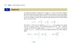
244, , Chapter 3 Applications of the Derivative, , 3.1, , Extrema of Functions, Absolute Extrema of Functions, The graph of the function f in Figure 1 gives the altitude of a hot-air balloon over the, time interval I  [a, d]. The point (c, f(c)), the lowest point on the graph of f, tells us, that the hot-air balloon attains its minimum altitude, f(c), at time t  c. The smallest, value attained by f for all values of t in the domain I of f, f(c), is called the absolute minimum value of f on I. Similarly, the point (d, f(d)), the highest point on the graph of f,, tells us that the balloon attains its maximum altitude, f(d), at time t  d. The largest value, attained by f for all values of t in I is called the absolute maximum value of f on I., y (ft), , (d, f (d)), , (c, f (c)), , FIGURE 1, The altitude f(t) of a hot-air, balloon for a  t  d, , 0, , a, , b, , c, , d, , t (hr), , More generally, we have the following definitions., , DEFINITIONS Extrema of a Function f, A function f has an absolute maximum at c if f(x)  f(c) for all x in the domain, D of f. The number f(c) is called the maximum value of f on D. Similarly, f, has an absolute minimum at c if f(x)  f(c) for all x in D. The number f(c) is, called the minimum value of f on D. The absolute maximum and absolute minimum values of f on D are called the extreme values, or extrema, of f on D., , EXAMPLE 1 Find the extrema of the function, if any, by examining its graph., a. f(x)  x 2, Solution, y, , b. t(x)  x 2, , c. h(x) , , 1, x, , d. k(x) , , 2x  7, The graphs of the functions f, t, h, and k are shown in Figure 2., y, , y, , y, , y  x2, 1, y  x_, x, , x, , 0, , y1, , x, y  _______, √x2  7, , 0, 0, , x, , 0, , FIGURE 2, , (b) t has a maximum at 0., , x, y  1, , y  x 2, , (a) f has a minimum at 0., , x, 2, , (c) h has no extrema., , (d) k has no extrema.

Page 3 :
3.1, , Extrema of Functions, , 245, , a. f has a minimum value of 0 at 0. Next, since the values of f are not bounded, above, f has no maximum value., b. t has a maximum value of 0 at 0. Also, because the values of t are not bounded, below, t has no minimum value., c. The values of h are neither bounded above nor bounded below, so h has no, absolute extrema., d. As x gets larger and larger, k(x) gets closer and closer to 1. But this value is, never attained; that is, a real number c does not exist such that k(c)  1. Therefore, k has no maximum value. Similarly, you can show that k has no minimum, value., , EXAMPLE 2 Find the extrema of the function:, a. f(x)  x 2, b. t(x)  x 2, , 1  x  2, 1  x  2, , Solution, a. The graph of f is shown in Figure 3a. We see that f has a minimum value of 0 at, 0. Next, observe that as x approaches 2 through values less than 2, f(x) increases, and approaches 4. But f never attains the value 4. Therefore, f does not have a, maximum., y, , y, , 4, , 4, y  x2, , y  x2, , 1, , 1, , FIGURE 3, , 1, , 1, , 2, , x, , (a) f has a minimum at 0., , 1, , 1, , 2, , x, , (b) t has a minimum at 0 and a maximum at 2., , b. The graph of t is shown in Figure 3b. As before, we see that t has a minimum, value of 0 at 0. Next, because 2 lies in the domain of t, we see that t does attain, a largest value, namely, t(2)  4., , Relative Extrema of Functions, If you refer once again to the graph of the function f giving the altitude of a hot-air, balloon over the interval [a, d] shown in Figure 4, you will see that the point (b, f(b)), is the highest point on the graph of f when compared to neighboring points. (For example, it is the highest point when compared to the points (t, f(t)), where a  t  c.) This, tells us that f(b) is the highest altitude attained by the balloon when considered over a, small time interval containing t  b. The value f(b) is called a relative (or local) maximum value of f.

Page 4 :
246, , Chapter 3 Applications of the Derivative, y (ft), (b, f (b)), , (c, f (c)), , FIGURE 4, The altitude of a hot-air, balloon for a  t  d, , 0, , a, , b, , c, , d, , t (hr), , Similarly, the point (c, f(c)) is the lowest point on the graph of f when compared, to points nearby. (For example, it is the lowest point when compared to the points, (t, f(t)), where b  t  d.) This tells us that the balloon attains the lowest altitude at, t  c when considered over a small time interval containing t  c. The value f(c) is, called a relative (or local) minimum value of f. Recall that f(c) also happens to be the, (absolute) minimum value of f, as we observed earlier., More generally, we have the following definition., , DEFINITIONS Relative Extrema of a Function, A function f has a relative (or local) maximum at c if f(c)  f(x) for all values of x in some open interval containing c. Similarly, f has a relative (or local), minimum at c if f(c)  f(x) for all values of x in some open interval containing c., , The function f whose graph is shown in Figure 5 has a relative maximum at a and, at c and a relative minimum at b and at d. The graph of f suggests that at a point corresponding to a relative extremum of f, either the tangent line is horizontal or it does, not exist. Put another way, the values of x that correspond to these points are precisely, the numbers in the domain of f at which f ¿ is zero or f ¿ does not exist., y, , FIGURE 5, The function f has relative extrema, at a, b, c, and d. The tangent lines, at a and b are horizontal. There, are no tangent lines at c and d., , 0, , a, , b, , c, , d, , x, , These observations suggest the following theorem, which tells us where the relative extrema of a function may occur., , THEOREM 1 Fermat’s Theorem, If f has a relative extremum at c, then either f ¿(c)  0 or f ¿(c) does not exist.

Page 5 :
3.1, , Extrema of Functions, , 247, , PROOF First, suppose that f has a relative maximum at c. If f is not differentiable at, c, then there is nothing to prove. So let’s suppose that f ¿(c) exists. Since f has a relative maximum at c, there exists an open interval, I, such that f(x)  f(c) for all x in, I. This implies that if we pick h to be positive and sufficiently small (so that c  h lies, in I), then, f(c  h)  f(c), , or, , f(c  h)  f(c)  0, , Multiplying both sides of the latter inequality by 1>h, where h  0, we obtain, f(c  h)  f(c), 0, h, Taking the right-hand limit of both sides of this inequality gives, lim, , h→0, , f(c  h)  f(c),  lim0  0, h, h→0, , By Theorem 3 of Section 1.2, , Since f ¿(c) exists, we have, f(c  h)  f(c), f(c  h)  f(c),  lim, h→0, h, h→0, h, , f ¿(c)  lim, , and we have shown that f ¿(c)  0., Next, we pick h to be negative and sufficiently small (so that c  h lies in I). Then, f(c  h)  f(c), , or, , f(c  h)  f(c)  0, , Upon multiplying this last inequality by 1>h and reversing the direction of the inequality (because 1>h  0), we have, f ¿(c)  lim, , h→0, , f(c  h)  f(c), f(c  h)  f(c),  lim, 0, h, h→0, h, , Thus, we have shown that f ¿(c)  0 and f ¿(c)  0, simultaneously. Therefore, f ¿(c)  0., This proves the theorem for the case in which f has a relative maximum at c. The, case in which f has a relative minimum at c can be proved in a similar manner (see, Exercise 90)., The values of x at which f ¿ is zero or f ¿ does not exist are given a special name., , DEFINITION Critical Number of f, A critical number of a function f is any number c in the domain of f at which, f ¿(c)  0 or f ¿(c) does not exist., , !, , Theorem 1 states that a relative extremum of f can occur only at a critical number, of f. It is important to realize, however, that the converse of Theorem 1 is false. In, other words, you may not conclude that if c is a critical number of f, then f must, have a relative extremum at c. (See Example 3.), , EXAMPLE 3 Show that zero is a critical number of each of the functions f(x)  x 3, and t(x)  x 1>3 but that neither function has a relative extremum at 0.

Page 6 :
248, , Chapter 3 Applications of the Derivative, , Solution The graphs of f and t are shown in Figure 6. Since f ¿(x)  3x 2  0 if x  0,, we see that 0 is a critical number of f. But observe that f(x)  0 if x  0 and f(x)  0, if x  0, and this tells us that f cannot have a relative extremum at 0., y, , y, , 1, , 1, y  x3, , 0, , 1, , FIGURE 6, Both f and t have 0 as a critical, number, but neither function, has a relative extremum at 0., , 1, , x, , y  x 1/3, , 0, , 1, , 1, , 1, , x, , 1, (b) The graph of t, , (a) The graph of f, , Next, we compute, t¿(x) , , 1 2>3, 1, x,  2>3, 3, 3x, , Note that t¿ is not defined at 0, but t is; so 0 is a critical number of t. Observe that, t(x)  0 if x  0 and t(x)  0 if x  0, so t cannot have a relative extremum at 0., , EXAMPLE 4 Find the critical numbers of f(x)  x  3x 1>3., Solution, , The derivative of f is, f ¿(x)  1  x 2>3 , , x 2>3  1, x 2>3, , Observe that f ¿ is not defined at 0 and also f ¿(x)  0 if x , cal numbers of f are 1, 0, and 1., , 1. Therefore, the criti-, , We will develop a systematic method for finding the relative extrema of a function, in Section 3.3. For the rest of this section we will develop techniques for finding the, extrema of continuous functions defined on closed intervals., , Finding the Extreme Values of a Continuous, Function on a Closed Interval, As you saw in the preceding examples, an arbitrary function might or might not have, a maximum value or a minimum value. But there is an important case in which the, extrema always exist for a function. The conditions are spelled out in Theorem 2., , THEOREM 2 The Extreme Value Theorem, If f is continuous on a closed interval [a, b], then f attains an absolute maximum, value f(c) for some number c in [a, b] and an absolute minimum value f(d) for, some number d in [a, b].

Page 7 :
3.1, , 249, , Extrema of Functions, , In certain applications, not only is a function continuous on a closed interval, [a, b], but it is also differentiable, with the possible exception of a finite set of numbers, on the open interval (a, b). In such cases, the following procedure can be used to, find the extrema of the function., , Guidelines for Finding the Extrema of a Continuous Function f on [a, b], 1. Find the critical numbers of f that lie in (a, b)., 2. Compute the value of f at each of these critical numbers, and also compute, f(a) and f(b)., 3. The absolute maximum value of f and the absolute minimum value of f are, precisely the largest and the smallest numbers found in Step 2., , This procedure can be justified as follows: If an extremum of f occurs at a number, in the open interval (a, b) , then it must also be a relative extremum of f ; hence it must, occur at a critical number of f. Otherwise, the extremum of f must occur at one or both, of the endpoints of the interval [a, b]. (See Figure 7.), y, , 0, , y, , a, , b, , x, , 0, , (a) The extreme values of f occur at the, endpoints., , y, , a, , b, , x, , (b) The extreme values of f occur at critical, numbers., , 0, , a, , b, , x, , (c) The absolute minimum value of f, occurs at both an endpoint and a critical, number of f , whereas the absolute, maximum value of f occurs at an, endpoint., , FIGURE 7, f is continuous on [a, b]., , EXAMPLE 5 Find the extreme values of the function f(x)  3x 4  4x 3  8 on, [1, 2]., Solution Since f is a polynomial function, it is continuous everywhere; in particular,, it is continuous on the closed interval [1, 2]. Therefore, we can use the Extreme Value, Theorem., First, we find the critical numbers of f in (1, 2):, f ¿(x)  12x 3  12x 2,  12x 2 (x  1), Observe that f ¿ is continuous on (1, 2). Next, setting f ¿(x)  0 gives x  0 or, x  1. Therefore, 0 and 1 are the only critical numbers of f in (1, 2).

Page 8 :
250, , Chapter 3 Applications of the Derivative, , Next, we compute f(x) at these critical numbers as well as at the endpoints 1 and, 2. These values are shown in the following table., , y, f (x)  3x4  4x 3  8, , (2, 8), , 4, , (1, 1), , 1, , x, , 2, , x, , 1, , 0, , 1, , 2, , f(x), , 1, , 8, , 9, , 8, , From the table we see that f attains the absolute maximum value of 8 at 2 and the, absolute minimum value of 9 at 1. The graph of f shown in Figure 8 confirms our, results. (You don’t need to draw the graph to solve the problem.), , (0, 8), (1, 9), , FIGURE 8, The maximum value of f is 8, and the, minimum value is 9., , EXAMPLE 6 Find the extreme values of the function f(x)  2 cos x  x on, [0, 2p]., Solution The function f is continuous everywhere; in particular, it is continuous on, the closed interval [0, 2p]. Therefore, the Extreme Value Theorem is applicable., First, we find the critical numbers of f in (0, 2p). We have, f ¿(x)  2 sin x  1, Observe that f ¿ is continuous on (0, 2p). Setting f ¿(x)  0 gives, 2 sin x  1  0, sin x  , , 1, 2, , Thus, x  7p>6 or 11p>6. (Remember x lies in (0, 2p).) So 7p>6 and 11p>6 are the, only critical numbers of f in (0, 2p)., Next, we compute the values of f at these critical numbers as well as at the endpoints 0 and 2p. These values are shown in the following table., 2, 0, , 2π, , x, , 0, , 7p, 6, , 11p, 6, , 2p, , f(x), , 2, , 5.40, , 4.03, , 4.28, , 6, , FIGURE 9, The graph of f(x)  2 cos x  x, on [0, 2p], , From the table we see that f attains the absolute maximum value of 2 at 0 and the, absolute minimum value of approximately 5.4 at 7p>6. The graph of f shown in Figure 9 confirms our results., , An Optimization Problem, The solution to many practical problems involves finding the absolute maximum or the, absolute minimum of a function. If we know that the function to be optimized is continuous on a closed interval, then the techniques of this section can be used to solve, the problem, as illustrated in the following example.

Page 9 :
3.1, , Extrema of Functions, , 251, , EXAMPLE 7 Maximum Deflection of a Beam Figure 10 depicts a beam of length L, and uniform weight w per unit length that is rigidly fixed at one end and simply supported at the other. An equation of the elastic curve (the dashed curve in the figure) is, y, , w, (2x 4  5Lx 3  3L2x 2), 48EI, , where the product EI is a constant called the flexural rigidity of the beam. Show, that the maximum deflection (the displacement of the elastic curve from the x-axis), occurs at x  (15  133)L>16 ⬇ 0.578L and has a magnitude of approximately, 0.0054wL4>(EI)., , L, , FIGURE 10, The beam is rigidly fixed at x  0, and simply supported at x  L., Note the orientation of the y-axis., , x, , 0, y, , Solution We wish to find the value of x on the closed interval [0, L] at which the, function f defined by, w, (2x 4  5Lx 3  3L2x 2), 48EI, , f(x) , , attains its absolute maximum value. Since f is continuous on [0, L], this value must be, attained at a critical number of f in (0, L) or at an endpoint of the interval. To find the, critical numbers of f, we compute, f ¿(x) , , w, (8x 3  15Lx 2  6L2x), 48EI, , , , w, x(8x 2  15Lx  6L2), 48EI, , Setting f ¿(x)  0 gives x  0 or, x, , 15L, , , , 15L, , 2225L2  192L2, 16, 133L, 16, , Because (15  133)L>16  L, we see that the sole critical number of f in (0, L), is x  (15  133)L>16 ⬇ 0.578L. Evaluating f at 0, 0.578L, and L, we obtain the, following table of values., f(0), 0, , f(0.578L), 0.0054wL, EI, , f(L), , 4, , 0, , We conclude that the maximum deflection occurs at x  (15  133)L>16 ⬇ 0.578L, and has a magnitude of approximately 0.0054wL4>(EI).

Page 10 :
252, , Chapter 3 Applications of the Derivative, , Our final example shows how a graphing utility can be used to approximate the, maximum and minimum values of a continuous function defined on a closed interval., But to obtain the exact values, we must solve the problem analytically., , EXAMPLE 8 Let f(x)  2 sin x  sin 2x., a. Use a graphing utility to plot the graph of f using the viewing window, C0, 3p, [3, 3]. Find the approximate absolute maximum and absolute mini2 D, mum values of f on the interval C0, 3p, 2 D., b. Obtain the exact absolute maximum and absolute minimum values of f analytically., , 3, , 3π, __, 2, , 0, , Solution, a. The required graph is shown in Figure 11. From the graph we see that the, absolute maximum value of f is approximately 2.6 obtained when x ⬇ 1. The, absolute minimum value of f is 2 obtained when x  3p>2., b. The function f is continuous everywhere and, in particular, on the interval C0, 3p, 2 D., We find, f ¿(x)  2 cos x  2 cos 2x, , 3, , FIGURE 11, ,  2 cos x  2(cos2 x  sin2 x), , cos 2x  cos2 x  sin2 x, ,  2 cos x  2(cos2 x  1  cos2 x), , sin2 x  1  cos2 x, ,  2(2 cos2 x  cos x  1), Since, 2 cos2 x  cos x  1  (2 cos x  1)(cos x  1)  0, if cos x  1 or 12, we see that x  p>3 or p. From the following table we see, that the absolute maximum value of f is 313>2 and the absolute minimum value, of f is 2., , 3.1, , x, , 0, , p, 3, , p, , 3p, 2, , f(x), , 0, , 313, 2, , 0, , 2, , CONCEPT QUESTIONS, , 1. Explain each of the following terms: (a) absolute maximum, value of a function f; (b) relative maximum value of a function f. Illustrate each with an example., 2. a. What is a critical number of a function f?, b. Explain the role of a critical number in determining the, relative extrema of a function., , 3. a. Explain the Extreme Value Theorem in your own words., b. Describe a procedure for finding the extrema of a continuous function f on a closed interval [a, b].

Page 11 :
3.1, , 3.1, , Extrema of Functions, , 253, , EXERCISES, 6. f defined on (1, ⬁), , In Exercises 1–6, you are given the graph of a function f defined, on the indicated domain. Find the absolute maximum and, absolute minimum values of f (if they exist) and where they are, attained., , y, , 2. f defined on (⬁, ⬁), , 1. f defined on (0, 2], y, , 1, , y, 1, , 3, , 1, , x, , 1, , 2, 1, 1, 3 2 1, 1, , 1 2 3, , 2 x, , 1, , x, , In Exercises 7–24, sketch the graph of the function and find its, absolute maximum and absolute minimum values, if any., 7. f(x)  2x  3 on [1, ⬁), , 2, , 9. h(t)  t  1 on (1, 0), 2, , 11. t(x)  x  1 on (0, ⬁), 2, , 3. f defined on (⬁, ⬁), , 15. f(x) , , 4 3 2 1, , 1, , 2, , 3, , 4, , 4. f defined on (2, ⬁), , x, , 3, 2, , 1, , 2, , 3, , x, , 5. f defined on [0, 5], y, , 1, on (0, 1], x, , 16. t(x) , , 17. f(x)  冟 x 冟 on [2, 1), 19. f(t)  2 sin t on 1 0,, 21., , y, , 2, f(u)  tan u on 1 p4 , p2 2, 3p, 2, , 20. h(t)  cos pt on C 14, 1 2, , 22. t(u)  sec u on Cp3 , p2 2, , x, if 1  x  0, 2  x if 0  x  2, , 24. f(x)  e, , 24  x 2, 24  x 2, , if 2  x  0, if 0  x  2, , In Exercises 25–42, find the critical number(s), if any, of the, function., 25. f(x)  2x  3, , 26. t(x)  4  3x, , 27. f(x)  2x 2  4x, , 28. h(t)  6t 2  t  2, , 29. f(x)  x 3  6x  2, , 30. t(t)  2t 3  3t 2  12t  4, , 31. f(x)  2x 3  6x  7, (1, 37), , 32. f(x) , , 1 3 1 2, x  x  2x  3, 3, 2, , 33. h(x)  x 4  4x 3  12, , 20, , 34. t(t)  3t 4  4t 3  12t 2  8, , 10, , 35. f(x)  3x 4  8x 3  6x 2  24x  10, 1, , 2, , 3, , 4, , x, (5, 5), , 1, on (1, 1), x, , 18. t(x)  冟 2x  1 冟 on (0, 2], , 23. f(x)  e, , 30, , 10, , 12. h(x)  x 2  1 on (2, 1], , 14. t(x)  2x 2  3x  1 on [0, 1), , 1, , 40, , 10. f(t)  t 2  1 on [1, 0), , 13. f(x)  x 2  4x  3 on (⬁, ⬁), , y, , 2 1, 1, 2, , 8. t(x)  3x  2 on (1, 2], , 36. h(z)  z 5  5z 3  10z  4, 37. f(x)  x 2>3, 38. t(t)  4t 1>3  3t 4>3, , V Videos for selected exercises are available online at www.academic.cengage.com/login.

Page 12 :
254, , Chapter 3 Applications of the Derivative, , 39. h(u) , , u, , 40. t(x) , , u 1, 2, , 41. f(t)  cos2(2t), , x2, x 3, 2, , 42. t(u)  2 sin u  cos 2u, , In Exercises 43–60, find the absolute maximum and absolute, minimum values, if any, of the function., 43. f(x)  x 2  x  2 on [0, 2], 44. f(x)  x 2  4x  3 on [1, 3], , 47. t(x)  3x 4  4x 3  1 on [2, 1], , 50. t(u) , 51. t(√) , , Source: Journal of the American Medical Association., , 8 3, x  8x 2  12 on [2, 3], 3, , x, x 1, 2, , 1u, u2  1, , on [1, 2], on [0, 2], , √, on [2, 4], √1, , 52. f(x)  2x , , 1, on [1, 3], x, , 53. f(x)  x  2 1x on [0, 9], 54. f(t) , , 1 2, t  4 1t on [0, 9], 8, , 65. Brain Growth and IQs In a study conducted at the National, Institute of Mental Health, researchers followed the development of the cortex, the thinking part of the brain, in, 307 children. Using repeated magnetic resonance imaging, scans from childhood to the late teens, they measured the, thickness (in millimeters) of the cortex of children of age, t years with the highest IQs: 121 to 149. These data lead, to the model, S(t)  0.000989t 3  0.0486t 2  0.7116t  1.46, 5  t  19, Show that the cortex of children with superior intelligence, reaches maximum thickness around age 11., , 55. f(x)  x 2>3 (x 2  4) on [1, 2], , Source: Nature., , 56. t(x)  x24  x 2 on [0, 2], , 66. Brain Growth and IQs Refer to Exercise 65. The researchers at, the institute also measured the thickness (also in millimeters) of the cortex of children of age t years who were of, average intelligence. These data lead to the model, , 57. f(x)  2  3 sin 2x on C0, p2 D, , 58. t(x)  cos x  sin x on [0, 2p], 59. t(t)  2 sin t  t on C0, p2 D, , A(t)  0.00005t 3  0.000826t 2  0.0153t  4.55, 5  t  19, , 60. f(x)  x  sin x on [0, 2p], 61. Maximizing Profit The total daily profit in dollars realized by, the TKK Corporation in the manufacture and sale of x dozen, recordable DVDs is given by the total profit function, P(x)  0.000001x 3  0.001x 2  5x  500, 0  x  2000, Find the level of production that will yield a maximum daily, profit., 62. Reaction to a Drug The strength of a human body’s reaction to, a dosage D of a certain drug is given by, k, D, RD a  b, 2, 3, 2, , where k is a positive constant. Show that the maximum reaction is achieved if the dosage is k units., 63. Traffic Flow The average speed of traffic flow on a stretch of, Route 124 between 6 A.M. and 10 A.M. on a typical weekday, is approximated by the function, f(t)  20t  401t  50, , 0t9, , where t is measured in decades with t = 0 corresponding to, the beginning of 1910. Show that the percentage of foreignborn medical residents was lowest in early 1970., , 46. f(t)  2t 3  3t 2  12t  3 on [2, 3], , 49. f(x) , , 64. Foreign-Born Medical Residents The percentage of foreign-born, medical residents in the United States from the beginning, of 1910 to the beginning of 2000 is approximated by the, function, P(t)  0.04363t 3  0.267t 2  1.59t  14.7, , 45. h(x)  x 3  3x 2  1 on [3, 2], , 48. f(x)  2x 4 , , where f(t) is measured in miles per hour and t is measured, in hours, with t  0 corresponding to 6 A.M. At what time in, the morning is the average speed of traffic flow highest? At, what time in the morning is it lowest?, , 0t4, , Show that the cortex of children with average intelligence, reaches maximum thickness at age 6., Source: Nature., , 67. Maximizing Revenue The quantity demanded per month of the, Peget wristwatch is related to the unit price by the demand, equation, p, , 50, 0.01x 2  1, , 0  x  20, , where p is measured in dollars and x is measured in units of, a thousand. How many watches must be sold by the manufacturer to maximize its revenue?, Hint: Recall that the revenue R  px., , 68. Poiseuille’s Law According to Poiseuille’s Law, the velocity, (in centimeters per second) of blood r cm from the central, axis of an artery is given by, √(r)  k(R2  r 2), , 0rR

Page 13 :
3.1, where k is a constant and R is the radius of the artery. Show, that the flow of blood is fastest along the central axis. Where, is the flow of blood slowest?, R, , 72. Air Pollution According to the South Coast Air Quality Management district, the level of nitrogen dioxide, a brown gas, that impairs breathing, that is present in the atmosphere, between 7 A.M. and 2 P.M. on a certain May day in downtown Los Angeles is approximated by, I(t)  0.03t 3(t  7)4  60.2, , 69. Chemical Reaction In an autocatalytic chemical reaction the, product formed acts as a catalyst for the reaction. If Q is the, amount of the original substrate that is present initially and, x is the amount of catalyst formed, then the rate of change, of the chemical reaction with respect to the amount of catalyst present in the reaction is, R(x)  kx(Q  x), , 0xQ, , where k is a constant. Show that the rate of the chemical, reaction is greatest at the point at which exactly half of the, original substrate has been transformed., 70. Velocity of Airflow During a Cough When a person coughs, the, trachea (windpipe) contracts, allowing air to be expelled at a, maximum velocity. It can be shown that the velocity √ of, airflow during a cough is given by, √  f(r)  kr 2(R  r), , 0rR, , where r is the radius of the trachea in centimeters during, a cough, R is the normal radius of the trachea in centimeters, and k is a constant that depends on the length of the, trachea. Find the radius for which the velocity of airflow, is greatest., 71. A Mixture Problem A tank initially contains 10 gal of brine, with 2 lb of salt. Brine with 1.5 lb of salt per gallon enters, the tank at the rate of 3 gal/min, and the well-stirred mixture, leaves the tank at the rate of 4 gal/min. It can be shown that, the amount of salt in the tank after t min is x lb, where, x  f(t)  1.5(10  t)  0.0013(10  t)4, , 255, , Extrema of Functions, , 0t7, , where I(t) is measured in pollutant standard index (PSI) and, t is measured in hours, with t  0 corresponding to 7 A.M., Determine the time of day when the PSI is the lowest and, when it is the highest., Source: The Los Angeles Times., , 73. Office Rents After the economy softened, the sky-high office, space rents of the late 1990s started to come down to earth., The function R gives the approximate price per square foot, in dollars, R(t), of prime space in Boston’s Back Bay and, Financial District from the beginning of 1997 (t  0) to the, beginning of 2002 (t  5), where, R(t)  0.711t 3  3.76t 2  0.2t  36.5, , 0t5, , Show that the office space rents peaked at about the middle, of the year 2000. What was the highest office space rent, during the period in question?, Source: Meredith & Grew Inc./Oncor., , 74. Maximum Deflection of a Beam A uniform beam of length L ft, and negligible weight rests on supports at both ends. When, subjected to a uniform load of w0 lb/ft, it bends and has the, elastic curve (the dashed curve in the figure below) described, by the equation, y, , w0, (x 4  2Lx 3  L3x), 24EI, , 0xL, , where the product EI is a constant called the flexural rigidity, of the beam. Show that the maximum deflection of the beam, occurs at the midpoint of the beam and that its value is, 5w0L4>(384EI) ., , 0  t  10, , What is the maximum amount of salt present in the tank at, any time?, , 0, , L, x (ft), , y (ft), , 75. Use of Diesel Engines Diesel engines are popular in cars in, Europe, where fuel prices are high. The percentage of new, vehicles in Western Europe equipped with diesel engines is, approximated by the function, f(t)  0.3t 4  2.58t 3  8.11t 2  7.71t  23.75, 0t4, where t is measured in years, with t  0 corresponding to, the beginning of 1996.

Page 14 :
256, , Chapter 3 Applications of the Derivative, a. Plot the graph of f using the viewing window, [0, 4] [0, 40]., b. What was the lowest percentage of new vehicles, equipped with diesel engines for the period in question?, , y (%), 100, , y  P(t), , Source: German Automobile Industry Association., , 76. Federal Debt According to data obtained from the Congressional Budget Office, the national debt (in trillions of dollars) is given by the function, f(t)  0.0022t 3  0.0465t 2  0.506t  3.27, , 75, P, 0, , 0  t  20, , where t is measured in years, with t  0 corresponding to, the beginning of 1990., a. Plot the graph of f using the viewing window, [0, 20] [0, 14]., b. When was the federal debt at the highest level over the, period under consideration? What was that level?, , 79. Path of a Boat A boat leaves the point O (the origin) located, on one bank of a river, traveling with a constant speed of, 20 mph and always heading toward a dock located at the, point A (1000, 0), which is due east of the origin (see the, figure). The river flows north at a constant speed of 5 mph., It can be shown that the path of the boat is, y  500 c a, , Source: Congressional Budget Office., , 77. A cylindrical tank of height h is filled with water. Suppose a, jet of water flows through an orifice on the tank. According, to Torricelli’s law, the velocity of flow of the jet of water is, given by V  12tx where t is the gravitational constant. It, can be shown that the range R (in feet) of the jet of water is, given by R  2 1x(h  x). Where should the orifice be, located so that the jet of water will have the maximum, range?, , t (days), , 1000  x 3>4, 1000  x 5>4, b a, b d, 1000, 1000, 0  x  1000, , Find the maximum distance the boat has drifted north during, its trip., y (ft), N, W, , E, S, , x, h, , O, R, , 78. Water Pollution When organic waste is dumped into a pond,, the oxidation process that takes place reduces the pond’s, oxygen content. However, given time, nature will restore, the oxygen content to its natural level. In the accompanying, graph, P(t) gives the oxygen content (as a percentage of its, normal level) t days after organic waste has been dumped, into the pond. Suppose that the oxygen content t days after, the organic waste has been dumped into the pond is given by, P(t)  100 a, , t 2  10t  100, t 2  20t  100, , b, , percent of its normal level. Find the coordinates of the point, P, and explain its significance., , A (1000, 0), , x (ft), , 80. Construction of an AC Transformer In constructing an AC transformer, a cross-shaped iron core is inserted into a coil (see, the figure). If the radius of the coil is a, find the values of x, and y such that the iron core has the largest surface area., Hint: Let x  a cos u and y  a sin u. Then maximize the function, S  4xy  4y(x  y)  8xy  4y 2,  4a 2 (sin 2u  sin2 u), on the interval 0  u , , p, 4., , a, q, x, , y

Page 15 :
3.1, 81. A body of mass m moves in an elliptical path with a constant angular speed v (see the figure). It can be shown that, the force acting on the body is always directed toward the, origin and has magnitude given by, F  mv 2a cos vt  b sin vt, 2, , 2, , 2, , 2, , 2, , where the product EI is a constant called the flexural rigidity, of the beam. Find the maximum deflection of the beam., Hint: Maximize y  f(x) over each interval [0, 1] and [1, 3] separately. Then combine your results., , t0, , where a and b are constants with a  b. Find the points on, the path where the force is greatest and where it is smallest., Does your result agree with your intuition?, , 257, , Extrema of Functions, , W, 3, , 0, 1, , x (ft), , y, y (ft), , b, a, , 84. Let, a x, , 0, , f(x)  e, , b, , 82. The object shown in the figure is a crate full of office equipment that weighs W lb. Suppose you try to move the crate, by tying a rope around it and pulling on the rope at an angle, u to the horizontal. Then the magnitude F of the force that, is required to set the crate in motion is, mW, F, m sin u  cos u, , 0u, , Show that f is discontinuous at x  0 but attains an absolute, maximum value and an absolute minimum value on [1, 1]., Does this contradict the Extreme Value Theorem?, 85. Let, f(x)  e, , p, 2, , where m is a constant called the coefficient of static friction., a. Find the angle u at which F is minimized., b. What is the magnitude of the force found in part (a)?, c. Suppose W  60 and m  0.4. Plot the graph of F as a, function of u on the interval C0, p2 D . Then verify the result, obtained in parts (a) and (b) for this special case., , x, if 1  x  0, x  1 if 0  x  1, , x2  1, 2, , if 1  x  2, if 2  x  4, , Show that f attains an absolute maximum value and an, absolute minimum value on the open interval (1, 4). Does, this contradict the Extreme Value Theorem?, 86. Show that the function f(x)  x 3  x  1 has no relative, extrema on (⬁, ⬁)., 87. Find the critical numbers of the greatest integer function, f(x)  Œ xœ ., 88. Find the absolute maximum value and the absolute minimum value (if any) of the function t(x)  x  Œ xœ , where, f(x)  Œxœ is the greatest integer function., , 89. Show that the function f(x)  sin(1>x) has infinitely many, critical numbers in any open interval that contains the origin., 90. a. Suppose f has a relative minimum at c. Show that the, function t defined by t(x)  f(x) has a relative maximum at c., b. Use the result of (a) to prove Theorem 1 for the case in, which f has a relative minimum at c., , q, , 83. A uniform beam of length 3 ft and negligible weight is supported at both ends. When subjected to a concentrated load, W at a distance 1 ft from one end, it bends and has the elastic curve (the dashed curve in the figure) described by the, equation, W, (5x  x 3), 9EI, yd, W, (x 3  9x 2  19x  3), 18EI, , if 0  x  1, if 1  x  3, , In Exercises 91–94, plot the graph of f and use the graph to estimate the absolute maximum and absolute minimum values of f in, the given interval., 91. f(x)  0.02x 5  0.3x 4  2x 3  6x  4 on [2, 2], 92. f(x)  0.3x 6  2x 4  3x 2  3 on [0, 2], 93. f(x) , 94. f(x) , , 0.2x 2, 3x  2x 2  1, 4, , on [0, 4], , x  cos x, on [0, 2], 1  0.5 sin x

Page 16 :
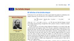
258, , Chapter 3 Applications of the Derivative, , In Exercises 95–98, (a) plot the graph of f in the given viewing, window and find the approximate absolute maximum and absolute, minimum values accurate to three decimal places, and (b) obtain, the exact absolute maximum and absolute minimum values of f, analytically., 95. f(x) , , 1 4 3, x  x  2 on [1, 2], 2, 2, , 96. f(x)  x  21  x 2 on [1, 1], 97. f(x) , , x1, on [0, 1], 1x  1, , 98. f(x)  2 sin x  x on C0, p2 D, , 3.2, , In Exercises 99–102, determine whether the statement is true or, false. If it is true, explain why it is true. If it is false, explain why, or give an example to show why it is false., 99. If f ¿(c)  0, then f has a relative maximum or a relative, minimum at c., 100. If f has a relative minimum at c, then f ¿(c)  0., , [0, 8], , 101. If f is defined on the closed interval [a, b], then f has an, absolute minimum value in [a, b]., , [2, 2], , 102. If f is continuous on the interval (a, b), then f attains an, absolute minimum value at some number c in (a, b)., , [0.8, 1], [0, 1], , The Mean Value Theorem, Rolle’s Theorem, The graph of the function f shown in Figure 1 gives the depth of a radical new twinpiloted submarine during a test dive. The submarine is on the surface at t  a [ f(a)  0], when it commences its dive. It resurfaces at t  b [ f(b)  0], the end of the test run., As you can see from the graph of f, there is at least one point on the graph of f at which, the tangent line to the curve is horizontal., y (ft), , Historical Biography, MICHEL ROLLE, (1652–1719), It is interesting to note that the theorem, that bears Michel Rolle’s name—which was, originally included in a 1691 book on geometry and algebra—is the basis for so many, concepts in calculus, given that Rolle himself was skeptical of the topic’s validity., Rolle attacked as a set of untruths what, were then the newly developing infinitesimal methods, now known as calculus. Eventually convinced of the validity of calculus, by Pierre Varignon (1654–1722), Rolle later, voiced his support for the subject. Shortly, thereafter, the general opposition to calculus collapsed, followed by many new, advances in the content area. Rolle’s Theorem is now found in the development of, many of the introductory topics of differential calculus., , 0, , a, , b, , t (min), , FIGURE 1, f(t) gives the depth of the submarine at time t., , We can convince ourselves that there must exist at least one such point on the graph, of f through the following intuitive argument: Since we know that the submarine, returned to the surface, there must be at least one point on the graph of f that corresponds to the time when the submarine stops diving and begins to resurface. The tangent line to the graph of f at this point must be horizontal., A mathematical description of this phenomenon is contained in Rolle’s Theorem,, named in honor of the French mathematician Michel Rolle (1652–1719)., , THEOREM 1 Rolle’s Theorem, Let f be continuous on [a, b] and differentiable on (a, b). If f(a)  f(b), then, there exists at least one number c in (a, b) such that f ¿(c)  0.

Page 17 :
3.2, , 259, , The Mean Value Theorem, , PROOF Let f(a)  f(b)  d. There are two cases to consider (see Figure 2)., y, y, , FIGURE 2, Geometric interpretations, of Rolle’s Theorem, , 0, , y = f(x), , y=d, , d, , a, , c1, , c2, , b, , d, , x, , (a) Case 1, , 0, , a, , c1, , c2, , b, , x, , (b) Case 2, , Case 1 f(x)  d for all x in [a, b] (see Figure 2a)., In this case, f ¿(x)  0 for all x in (a, b), so f ¿(c)  0 for any number c in (a, b)., Case 2 f(x) d for at least one x in [a, b] (see Figure 2b)., In this case there must be a number x in (a, b) where f(x)  d or f(x)  d. First, suppose that f(x)  d. Since f is continuous on [a, b], the Extreme Value Theorem implies, that f attains an absolute maximum value at some number c in [a, b]. The number c, cannot be an endpoint because f(a)  f(b)  d, and we have assumed that f(x)  d, for some number x in (a, b). Therefore, c must be in (a, b). Since f is differentiable on, (a, b), f ¿(c) exists, and by Fermat’s Theorem f ¿(c)  0., The proof for the case in which f(x)  d is similar and is left as an exercise (Exercise 39)., , EXAMPLE 1 Let f(x)  x 3  x for x in [1, 1]., a. Show that f satisfies the hypotheses of Rolle’s Theorem on [1, 1]., b. Find the number(s) c in (1, 1) such that f ¿(c)  0 as guaranteed by Rolle’s, Theorem., , y, 1, y  x3  x, , 1, , 3,  __, 3, , 0, , __3, , 1, , 3, , 1, , FIGURE 3, The numbers c1   13>3 and, c2  13>3 satisfy f ¿(c)  0 as, guaranteed by Rolle’s Theorem., , x, , Solution, a. The polynomial function f is continuous and differentiable on (⬁, ⬁). In particular, it is continuous on [1, 1] and differentiable on (1, 1). Furthermore,, f(1)  (1)3  (1)  0, , and, , f(1)  13  1  0, , and the hypotheses of Rolle’s theorem are satisfied., b. Rolle’s Theorem guarantees that there exists at least one number c in (1, 1), such that f ¿(c)  0. But f ¿(x)  3x 2  1, so to find c, we solve, 3c2  1  0, obtaining c  13>3. In other words, there are two numbers, c1   13>3 and, c2  13>3, in (1, 1) for which f ¿(c)  0 (Figure 3)., , EXAMPLE 2 A Real-Life Illustration of Rolle’s Theorem During a test dive of a prototype of a twin-piloted submarine, the depth in feet of the submarine at time t in minutes is given by h(t)  t 3(t  7)4, where 0  t  7., a. Use Rolle’s Theorem to show that there is some instant of time t  c between 0, and 7 when h¿(c)  0., b. Find the number c and interpret your results.

Page 18 :
260, , Chapter 3 Applications of the Derivative, , Solution, a. The polynomial function h is continuous on [0, 7] and differentiable on (0, 7)., Furthermore, h(0)  0 and h(7)  0, so the hypotheses of Rolle’s Theorem, are satisfied. Therefore, there exists at least one number c in (0, 7) such that, h¿(c)  0., b. To find the value of c, we first compute, h¿(t)  3t 2(t  7)4  t 3 (4)(t  7)3, , y (ft), 7000, ,  t 2(t  7)3[3(t  7)  4t], , (3, 6912), ,  7t 2(t  7)3(t  3), , y  t 3(t  7) 4, , 0, , 3, , 7, , t (min), , FIGURE 4, The submarine is at a depth of h(t) feet, at time t minutes., , Setting h¿(t)  0 gives t  0, 3, or 7. Since 3 is the only number in the interval, (0, 7) such that h¿(3)  0, we see that c  3. Interpreting our results, we see, that the submarine is on the surface initially (since h(0)  0) and returns to the, surface again after 7 minutes (since h(7)  0). The vertical component of the, velocity of the submarine is zero at t  3, at which time the submarine attains, the greatest depth of h(3)  33 (3  7)4  6912 ft. The graph of h is shown in, Figure 4., Rolle’s Theorem is a special case of a more general result known as the Mean Value, Theorem., , THEOREM 2 The Mean Value Theorem, Let f be continuous on [a, b] and differentiable on (a, b). Then there exists at, least one number c in (a, b) such that, f ¿(c) , , f(b)  f(a), ba, , (1), , To interpret this theorem geometrically, notice that the quotient in Equation (1) is, just the slope of the secant line passing through the points P(a, f(a)) and Q(b, f(b)), lying on the graph of f (Figure 5). The quantity f ¿(c) on the left, however, gives the, slope of the tangent line to the graph of f at x  c. The Mean Value Theorem tells us, that under suitable conditions on f, there is always at least one point (c, f(c)) on the, graph of f for a  c  b such that the tangent line to the graph of f at this point is, parallel to the secant line passing through P and Q. Observe that if f(a)  f(b), then, Theorem 2 reduces to Rolle’s Theorem., y, T, (c, f (c)), , S, Q(b, f (b)), , P(a, f (a)), , FIGURE 5, The tangent line T at (c, f(c)) is parallel, to the secant line S through P and Q., , 0, , a, , c, , b, , x

Page 19 :
3.2, , The Mean Value Theorem, , 261, , PROOF If you examine Figure 5, you will see that the vertical distance between the, graph of f and the secant line S passing through P and Q is maximal at x  c. This, observation gives a clue to the proof of the Mean Value Theorem: Find a function whose, absolute value gives the vertical distances between the graph of f and the secant line., Then optimize this function., Now an equation of the secant line can be found by using the point-slope form of, the equation of a line with slope [ f(b)  f(a)]>(b  a) and the point (b, f(b)). Thus,, y  f(b) , , f(b)  f(a), ⴢ (x  b), ba, , y  f(b) , , f(b)  f(a), ⴢ (x  b), ba, , or, , Define the function D by, D(x)  f(x)  cf(b) , , f(b)  f(a), ⴢ (x  b)d, ba, , (2), , Notice that 冟 D(x) 冟 gives the vertical distance between the graph of f and the secant line, through P and Q (Figure 6). The function D is continuous on [a, b] and differentiable, on (a, b), so we can use Rolle’s Theorem on D. First, we note that D(a)  D(b)  0., Therefore, there exists at least one number c in (a, b) such that D¿(c)  0. But, D¿(x)  f ¿(x) , , f(b)  f(a), ba, , so D¿(c)  0 implies that, 0  f ¿(c) , , f(b)  f(a), ba, , or, f ¿(c) , , f(b)  f(a), ba, , as was to be shown., y, , y, y  f (x), P(a, f (a)), , Q(b, f (b)), 冷 D(x)冷, y  f (b) , , y  f(b) , f (b)  f (a), ba, , y  f (x), , (x  b), , 冷 D(x)冷, , f (b)  f(a), ba, Q(b, f (b)), , P(a, f (a)), , 0, , x, , 0, , x, , FIGURE 6, 冟 D(x) 冟 gives the vertical distance between the graph of f and the secant line passing through P and Q., , (x  b)

Page 20 :
262, , Chapter 3 Applications of the Derivative, , EXAMPLE 3 Let f(x)  x 3., a. Show that f satisfies the hypotheses of the Mean Value Theorem on [1, 1]., b. Find the number(s) c in (1, 1) that satisfy Equation (1) as guaranteed by the, Mean Value Theorem., y, 1, , (1, f (1)), y  x3, , 3,  __, 3, , 1, , __3, , 1, , Solution, a. f is a polynomial function, so it is continuous and differentiable on (⬁, ⬁). In, particular, f is continuous on [1, 1] and differentiable on (1, 1). So the, hypotheses of the Mean Value Theorem are satisfied., b. f ¿(x)  3x 2, so f ¿(c)  3c2. With a  1 and b  1, Equation (1) gives, f(1)  f(1),  f ¿(c), 1  (1), , x, , 3, , or, 1, (1, f(1)), , FIGURE 7, The numbers c1   13>3 and, c2  13>3 satisfy Equation (1),, as guaranteed by the Mean Value, Theorem., , 1  (1),  3c2, 1  (1), 1  3c2, and c  13>3. So there are two numbers, c1   13>3 and c2  13>3, in, (1, 1) that satisfy Equation (1). (See Figure 7.), The next example gives an interpretation of the Mean Value Theorem in a real-life, setting., , EXAMPLE 4 The Mean Value Theorem and the Maglev The position of a maglev moving along a straight, elevated monorail track is given by s  f(t)  4t 2, 0  t  30,, where s is measured in feet and t is measured in seconds. Then the average velocity of, the maglev during the first 4 sec of the run is, f(4)  f(0), 64  0, ,  16, 40, 4, , (3), , or 16 ft/sec. Next, since f is continuous on [0, 4] and differentiable on (0, 4), the Mean, Value Theorem guarantees that there is a number c in (0, 4) such that, f(4)  f(0),  f ¿(c), 40, , (4), , But f ¿(t)  8t, so using Equation (3), we see that Equation (4) is equivalent to, 16  8c, or c  2. Since f ¿(t) measures the instantaneous velocity of the maglev at any time t,, the Mean Value Theorem tells us that at some time t between t  0 and t  4 (in this, case, t  2) the maglev must attain an instantaneous velocity equal to the average velocity of the maglev over the time interval [0, 4]., , Some Consequences of the Mean Value Theorem, An important application of the Mean Value Theorem is to establish other mathematical results. For example, we know that the derivative of a constant function is zero., Now we can show that the converse is also true.

Page 21 :
3.2, , The Mean Value Theorem, , 263, , THEOREM 3, If f ¿(x)  0 for all x in an interval (a, b), then f is constant on (a, b)., , PROOF Suppose that f ¿(x)  0 for all x in (a, b). To prove that f is constant on, (a, b), it suffices to show that f has the same value at every pair of numbers in (a, b)., So let x 1 and x 2 be arbitrary numbers in (a, b) with x 1  x 2. Since f is differentiable, on (a, b), it is also differentiable on (x 1, x 2) and continuous on [x 1, x 2]. Therefore, the, hypotheses of the Mean Value Theorem are satisfied on the interval [x 1, x 2]. Applying, the theorem, we see that there exists a number c in (x 1, x 2) such that, f ¿(c) , , f(x 2)  f(x 1), x2  x1, , (5), , But by hypothesis, f ¿(x)  0 for all x in (a, b), so f ¿(c)  0. Therefore, Equation (5), implies that f(x 2)  f(x 1)  0, or f(x 1)  f(x 2) ; that is, f has the same value at any, two numbers in (a, b). This completes the proof., , COROLLARY TO THEOREM 3, If f ¿(x)  t¿(x) for all x in an interval (a, b), then f and t differ by a constant on, (a, b); that is, there exists a constant c such that f(x)  t(x)  c for all x in, (a, b)., , PROOF Let h(x)  f(x)  t(x). Then, h¿(x)  f ¿(x)  t¿(x)  0, for every x in (a, b). By Theorem 3, h is constant; that is, f  t is constant on (a, b)., Thus, f(x)  t(x)  c for some constant c and f(x)  t(x)  c for all x in (a, b)., , Determining the Number of Zeros of a Function, Our final example brings together two important theorems—the Intermediate Value, Theorem and Rolle’s Theorem—to help us determine the number of zeros of a function f in a given interval [a, b]., , EXAMPLE 5 Show that the function f(x)  x 3  x  1 has exactly one zero in the, interval [2, 0]., , 10, , 2, , 2, , 10, , FIGURE 8, The graph shows the zero of f., , Solution First, observe that f is continuous on [2, 0] and that f(2)  9 and, f(0)  1. Therefore, by the Intermediate Value Theorem, there must exist at least one, number c that satisfies 2  c  0 such that f(c)  0. In other words, f has at least, one zero in (2, 0)., To show that f has exactly one zero, suppose, on the contrary, that f has at least two, distinct zeros, x 1 and x 2. Without loss of generality, suppose that x 1  x 2. Then, f(x 1)  f(x 2)  0. Because f is differentiable on (x 1, x 2), an application of Rolle’s Theorem tells us that there exists a number c between x 1 and x 2 such that f ¿(c)  0. But, f ¿(x)  3x 2  1  1 can never be zero in (x 1, x 2). This contradiction establishes the, result., The graph of f is shown in Figure 8.

Page 22 :
264, , Chapter 3 Applications of the Derivative, , 3.2, , CONCEPT QUESTIONS, y, , 1. State Rolle’s Theorem and give a geometric interpretation, of it., 2. State the Mean Value Theorem, and give a geometric interpretation of it., 3. Refer to the graph of f., a. Sketch the secant line through the points (0, 3) and, (9, 8) . Then draw all lines parallel to this secant line, that are tangent to the graph of f., b. Use the result of part (a) to estimate the values of c that, satisfy the Mean Value Theorem on the interval [0, 9]., , 8, 7, y  f (x), , 6, 5, 4, 3, 2, 1, 0, , 3.2, , 1, , 2, , 3, , 4, , 5, , 6, , 7, , 8, , 9, , 10, , x, , EXERCISES, altitude of the plane at time t (in minutes), where 0  t  30., Use Rolle’s Theorem to explain why there must be at least, one number c with 0  c  30 such that A¿(c)  0. Interpret, your result., , In Exercises 1–8, verify that the function satisfies the hypotheses, of Rolle’s Theorem on the given interval, and find all values of c, that satisfy the conclusion of the theorem., 1. f(x)  x 2  4x  3;, , [1, 3], , 18. Breaking the Speed Limit A trucker drove from Bismarck to, Fargo, a distance of 193 mi, in 2 hr and 55 min. Use the, Mean Value Theorem to show that the trucker must have, exceeded the posted speed limit of 65 mph at least once, during the trip., , 2. t(x)  x  9x; [3, 3], 3, , 3. f(x)  x  x  2x;, 3, , 2, , [2, 0], , 4. h(x)  x (x  7) ; [0, 7], 3, , 4, , 5. f(x)  x21  x 2; [1, 1], , 19. Test Flights In a test flight of the McCord Terrier, an experimental VTOL (vertical takeoff and landing) aircraft, it was, determined that t sec after takeoff, when the aircraft was, operated in the vertical takeoff mode, its altitude was, , 6. f(t)  t 2>3 (6  t)1>3; [0, 6], 7. h(t)  sin2 t;, , [0, p], , 8. f(x)  cos 2x  1;, , [0, p], , h(t) , , In Exercises 9–16, verify that the function satisfies the hypotheses of the Mean Value Theorem on the given interval, and find, all values of c that satisfy the conclusion of the theorem., 9. f(x)  x  1;, 2, , 1, 11. h(x)  ;, x, , 10. f(x)  x  2x ;, 3, , [0, 2], , 13. h(x)  x22x  1;, C0,, , 15. f(x)  x  sin x;, , p, 2D, , [0, 4], , C p2 ,, , pD, , sin t, 16. t(t) , ;, 1  cos t, , C0,, , 0t8, , Use Rolle’s Theorem to show that there exists a number c, satisfying 0  c  8 such that h¿(c)  0. Find the value of, c, and explain its significance., , [1, 2], , t, 12. t(t) , ; [2, 0], t1, , [1, 3], , 14. f(x)  sin x;, , 2, , 1 4, t  t 3  4t 2, 16, , 20. Hotel Occupancy The occupancy rate of the all-suite Wonderland Hotel, located near a theme park, is given by the function, , p, 2D, , 17. Flight of an Aircraft A commuter plane takes off from the Los, Angeles International Airport and touches down 30 min later, at the Ontario International Airport. Let A(t) (in feet) be the, , V Videos for selected exercises are available online at www.academic.cengage.com/login., , r(t) , , 10 3 10 2 200, t , t , t  56, 81, 3, 9, , 0  t  12, , where t is measured in months with t  0 corresponding to, the beginning of January. Show that there exists a number c, that satisfies 0  c  12 such that r¿(c)  0. Find the value, of c, and explain its significance.

Page 23 :
3.2, 21. Let f(x)  冟 x 冟  1. Show that there is no number c in, (1, 1) such that f ¿(c)  0 even though f(1)  f(1)  0., Why doesn’t this contradict Rolle’s Theorem?, 22. Let f(x)  1  x 2>3, a  1, and b  8. Show that there is, no number c in (a, b) such that, f ¿(c) , , f(b)  f(a), ba, , Doesn’t this contradict the Mean Value Theorem? Explain., 23. Let, f(x)  e, , x2, if x  1, 2  x if x  1, , Does f satisfy the hypotheses of the Mean Value Theorem on, [0, 2]? Explain., 24. Prove that f(x)  4x 3  4x  1 has at least one zero in the, interval (0, 1) ., Hint: Apply Rolle’s Theorem to the function t(x)  x 4  2x 2  x, on [0, 1]., , 25. Prove that f(x)  x 5  6x  4 has exactly one zero in, (⬁, ⬁)., 26. Prove that the equation x 7  6x 5  2x  6  0 has exactly, one real root., 27. Prove that the function f(x)  x  12x  c, where c is any, real number, has at most one zero in [0, 1]., 5, , 28. Use the Mean Value Theorem to prove that, 冟 sin a  sin b 冟  冟 a  b 冟 for all real numbers a and b., 29. Suppose that the equation, anx n  an1x n1  p  a1x  0, has a positive root r. Show that the equation, nanx n1  (n  1)an1x n2  p  a1  0, has a positive root smaller than r., Hint: Use Rolle’s Theorem., , 30. Suppose f ¿(x)  c, where c is a constant, for all values, of x. Show that f must be a linear function of the form, f(x)  cx  d for some constant d., Hint: Use the corollary to Theorem 3., , 31. Let f(x)  x 4  4x  1., a. Use Rolle’s Theorem to show that f has exactly two, distinct zeros., b. Plot the graph of f using the viewing window, [3, 3] [5, 5]., 32. Let, f(x)  •, , x sin, 0, , p, x, , if x  0, if x  0, , The Mean Value Theorem, , 265, , Use Rolle’s Theorem to prove that the derivative f ¿(x) is, equal to zero at an infinite set of numbers in the interval, (0, 1) . Plot the graph of f using the viewing window, [0, 1] [1, 1]., 33. Prove the formula, cos2 x , , 1  cos 2x, 2, , Hint: Let f(x)  cos2 x  12 cos 2x. Show that f ¿(x)  0 on (⬁, ⬁)., Use Theorem 3 to conclude that f(x)  C, where C is a constant., Determine C., , 34. Suppose that f and t are continuous on an interval [a, b] and, differentiable on the interval (a, b). Furthermore, suppose, that f(a)  t(a) and f ¿(x)  t¿(x) for a  x  b. Prove that, f(x)  t(x) for a  x  b., Hint: Apply the Mean Value Theorem to the function h  f  t., , 35. Let f(x)  Ax 2  Bx  C, and let [a, b] be an arbitrary, interval. Show that the number c in the Mean Value Theorem applied to the function f lies at the midpoint of the, interval [a, b]., 36. Let f(x)  2(x  1)(x  2)(x  3)(x  4). Prove that f ¿ has, exactly three real zeros., 37. A real number c such that f(c)  c is called a fixed point of, the function f. Geometrically, a fixed point of f is a point, that is mapped by f onto itself. Prove that if f is differentiable and f ¿(x) 1 for all x in an interval I, then f has at, most one fixed point in I., 38. Use the result of Exercise 37 to show that f(x)  1x  6, has exactly one fixed point in the interval (0, ⬁). What is, the fixed point?, 39. Complete the proof of Rolle’s Theorem by considering the, case in which f(x)  d for some number x in (a, b)., 40. Let f be continuous on [a, b] and differentiable on (a, b). Put, h  b  a., a. Use the Mean Value Theorem to show that there exists at, least one number u that satisfies 0  u  1 such that, f(a  h)  f(a),  f ¿(a  uh), h, b. Find u in the formula in part (a) for the function, f(x)  x 2., 41. Let f(x)  x 4  2x 3  x  2., a. Show that f satisfies the hypotheses of Rolle’s Theorem, on the interval [1, 2]., b. Use a calculator or a computer to estimate all values of c, accurate to five decimal places that satisfy the conclusion, of Rolle’s Theorem., c. Plot the graph of f and the (horizontal) tangent lines to, the graph of f at the point(s) (c, f(c)) for the values of c, found in part (b).

Page 24 :
266, , Chapter 3 Applications of the Derivative, , 42. Let f(x)  x 2 sin x., a. Show that f satisfies the hypotheses of Rolle’s Theorem, on the interval [0, p]., b. Use a calculator or a computer to estimate all value(s) of, c accurate to five decimal places that satisfy the conclusion of Rolle’s Theorem., c. Plot the graph of f and the (horizontal) tangent lines to, the graph of f at the point(s) (c, f(c)) for the value(s) of, c found in part (b)., , In Exercises 45–50, determine whether the statement is true or, false. If it is true, explain why it is true. If it is false, explain why, or give an example to show why it is false., 45. Suppose that f is continuous on [a, b] and differentiable, on (a, b). If f ¿(c)  0 for at least one c in (a, b), then, f(a)  f(b)., 46. Suppose that f is continuous on [a, b] but is not differentiable on (a, b). Then there does not exist a number c in, (a, b) such that, , 43. Let f(x)  x 4  2x 2  2., a. Use a calculator or a computer to estimate all values of, c accurate to three decimal places that satisfy the conclusion of the Mean Value Theorem for f on the interval, [0, 2]., b. Plot the graph of f, the secant line passing through the, points (0, 2) and (2, 10) , and the tangent line to the, graph of f at the point(s) (c, f(c)) for the value(s) of c, found in part (a)., , f ¿(c) , , 47. If f ¿(x)  0 for all x, then f is a constant function., 48. If 冟 f ¿(x) 冟  1 for all x, then, 冟 f(x 1)  f(x 2) 冟  冟 x 1  x 2 冟, for all numbers x 1 and x 2., , 44. Let f(x)  sin 1x., a. Use a calculator or a computer to estimate all values of, c accurate to three decimal places that satisfy the conclusion, of the Mean Value Theorem for f on the interval, 2, C0, p4 D ., b. Plot the graph of f, the secant line passing through the, 2, points (0, 0) and 1 p4 , 1 2 , and the tangent line to the graph, of f at the point(s) (c, f(c)) for the value(s) of c found in, part (b)., , 3.3, , f(b)  f(a), ba, , 49. There does not exist a continuous function defined on, the interval [2, 5] and differentiable on (2, 5) satisfying, 冟 f(5)  f(2) 冟  6 on [2, 5] and 冟 f ¿(x) 冟  2 for all x, in (2, 5)., 50. If f is continuous on [1, 3], differentiable on (1, 3), and satisfies f(1)  2, f(3)  5, then there exists a number c satisfying 1  c  3, such that f ¿(c)  32., , Increasing and Decreasing Functions and the First Derivative Test, Increasing and Decreasing Functions, Among the important factors in determining the structural integrity of an aircraft is its, age. Advancing age makes the parts of a plane more likely to crack. The graph of the, function f in Figure 1 is referred to as a “bathtub curve” in the airline industry. It gives, the fleet damage rate (damage due to corrosion, accident, and metal fatigue) of a typical fleet of commercial aircraft as a function of the number of years of service., , FIGURE 1, The “bathtub curve” gives the number, of planes in a fleet that are damaged as, a function of the age of the fleet., , Fleet damage rate, , y, , Economic life objective, 0, , 2, , 4, , 6, , 8 10 12 14 16 18 20 22 24, , t, , Years in service, , The function is decreasing on the interval (0, 4) , showing that the fleet damage rate, is dropping as problems are found and corrected during the initial shakedown period., The function is constant on the interval (4, 10) , reflecting that planes have few struc-

Page 25 :
3.3, , 267, , Increasing and Decreasing Functions and the First Derivative Test, , tural problems after the initial shakedown period. Beyond this, the function is increasing, reflecting an increase in structural defects due mainly to metal fatigue., These intuitive notions involving increasing and decreasing functions can be, described mathematically as follows., , DEFINITIONS Increasing and Decreasing Functions, A function f is increasing on an interval I, if for every pair of numbers x 1 and, x 2 in I,, x1  x2, , f(x 1)  f(x 2), , implies that, , See Figure 2a., , f is decreasing on I if, for every pair of numbers x 1 and x 2 in I,, x1  x2, , f(x 1)  f(x 2), , implies that, , See Figure 2b., , f is monotonic on I if it is either increasing or decreasing on I., , y, , y, y  f (x), f (x1), , f (x2), f (x2), , f (x1), , x1, , 0, , FIGURE 2, , x2, , x, , 0, , y  f (x), , x1, , x, , x2, , (b) f is decreasing on I., , (a) f is increasing on I., , Since the derivative of a function measures the rate of change of that function, it, lends itself naturally as a tool for determining the intervals where a differentiable function is increasing or decreasing. As you can see in Figure 3, if the graph of f has tangent lines with positive slopes over an interval, then the function is increasing on that, interval. Similarly, if the graph of f has tangent lines with negative slopes over an interval, then the function is decreasing on that interval. Also, we know that the slope of, the tangent line at (x, f(x)) and the rate of change of f at x are given by f ¿(x). Therefore, f is increasing on an interval where f ¿(x)  0 and decreasing on an interval where, f ¿(x)  0., y, , y  f (x), Slope is negative, , Slope is, positive, , FIGURE 3, f is increasing on an interval, where f ¿(x)  0 and decreasing, on an interval where f ¿(x)  0., , 0, , Slope is, positive, , x

Page 26 :
268, , Chapter 3 Applications of the Derivative, , These intuitive observations lead to the following theorem., , THEOREM 1 Suppose f is differentiable on an open interval (a, b)., a. If f ¿(x)  0 for all x in (a, b), then f is increasing on (a, b)., b. If f ¿(x)  0 for all x in (a, b), then f is decreasing on (a, b)., c. If f ¿(x)  0 for all x in (a, b), then f is constant on (a, b)., , PROOF, a. Let x 1 and x 2 be any two numbers in (a, b) with x 1  x 2. Since f is differentiable, on (a, b), it is continuous on [x 1, x 2] and differentiable on (x 1, x 2). By the Mean, Value Theorem, there exists a number c in (x 1, x 2) such that, f ¿(c) , , f(x 2)  f(x 1), x2  x1, , or, equivalently,, f(x 2)  f(x 1)  f ¿(c)(x 2  x 1), , (1), , Now, f ¿(c)  0 by assumption, and x 2  x 1  0 because x 1  x 2. Therefore,, f(x 2)  f(x 1)  0 , or f(x 1)  f(x 2) . This shows that f is increasing on (a, b)., b. The proof of (b) is similar and is left as an exercise (see Exercise 60)., c. This was proved in Theorem 3 in Section 3.2., Theorem 1 enables us to develop a procedure for finding the intervals where a function is increasing, decreasing, or constant. In this connection, recall that a function can, only change sign as we move across a zero or a number at which the function is discontinuous., , Determining the Intervals Where a Function Is Increasing or Decreasing, 1. Find all the values of x for which f ¿(x)  0 or f ¿(x) does not exist. Use, these values of x to partition the domain of f into open intervals., 2. Select a test number c in each interval found in Step 1, and determine the, sign of f ¿(c) in that interval., a. If f ¿(c)  0, then f is increasing on that interval., b. If f ¿(c)  0, then f is decreasing on that interval., c. If f ¿(c)  0, then f is constant on that interval., , EXAMPLE 1 Determine the intervals where the function f(x)  x 3  3x 2  2 is, increasing and where it is decreasing., Solution, , We first compute, f ¿(x)  3x 2  6x  3x(x  2), , from which we see that f ¿ is continuous everywhere and has zeros at 0 and 2. These, zeros of f ¿ partition the domain of f into the intervals (⬁, 0) , (0, 2) , and (2, ⬁) .

Page 27 :
3.3, , +++++++++ 0 – – – – – – – 0 ++++++, 0, , x, , 2, , FIGURE 4, The sign diagram for f ¿, y, , Increasing and Decreasing Functions and the First Derivative Test, , 269, , To determine the sign of f ¿(x) on each of these intervals, we evaluate f ¿(x) at a convenient test number in each interval. These results are summarized in the following, table., , y = x 3  3x 2  2, , 4, 3, 2, , Interval, , Test number c, , f ⴕ(c), , Sign of f ⴕ(c), , (⬁, 0), (0, 2), (2, ⬁), , 1, 1, 3, , 9, 3, 9, , , , , , 1, 2, , 1 1, , 1, , 2, , x, , 3, , 2, 3, , FIGURE 5, f is increasing on (⬁, 0), decreasing, on (0, 2), and increasing on (2, ⬁)., , Using these results, we obtain the sign diagram for f ¿(x) shown in Figure 4. We conclude that f is increasing on (⬁, 0) and (2, ⬁) and decreasing on (0, 2). The graph, of f is shown in Figure 5., , EXAMPLE 2 Determine the intervals where the function f(x)  x  1>x is increasing and where it is decreasing., Solution, , The derivative of f is, f ¿(x)  1 , , f not defined at x  0, + + + + + + + + 0– – – –0 + + + + + + + + +, 1, , 0, , x, , 1, , FIGURE 6, The sign diagram for f ¿, , 3, 2, , x, , 2, , , , (x  1)(x  1), x2, , 1, f ¿a b  3,, 2, , 1, f ¿a b  3,, 2, , and, , f ¿(2) , , 3, 4, , 1, y  x  x_, , 1, , FIGURE 7, The graph of f, , x2  1, , giving us the sign diagram of f ¿(x) shown in Figure 6. We conclude that f is increasing on (⬁, 1) and (1, ⬁) and decreasing on (1, 0) and (0, 1). The graph of f is, shown in Figure 7.* Note that f ¿(x) does not change sign as we move across the point, of discontinuity., , 4, , 4 3 2 1, 1, , x, , 2, , , , from which we see that f ¿(x) is continuous everywhere except at x  0 and has zeros, at x  1 and x  1. These values of x partition the domain of f into the intervals, (⬁, 1), (1, 0), (0, 1), and (1, ⬁). By evaluating f ¿(x) at each of the test numbers, x  2, 12, 12, and 2, we find, 3, f ¿(2)  ,, 4, , y, , 1, , 1, , 2, , 3, , 4, , x, , Finding the Relative Extrema of a Function, We will now see how the derivative of a function f can be used to help us find the relative extrema of f. If you examine Figure 8, you can see that the graph of f is rising to, the left of the relative maximum that occurs at b and falling to the right of it. Likewise, at the relative minima of f at a and d, you can see that the graph of f is falling, to the left of these critical numbers and rising to the right of them. Finally, look at the, behavior of the graph of f at the critical numbers c and e. These numbers do not give, rise to relative extrema. Notice that f is either increasing or decreasing on both sides, of these critical numbers., , *The graph of f approaches the dashed line as x →, be discussed in Section 3.6., , ⬁ . The dashed line is called a slant asymptote and will

Page 28 :
270, , Chapter 3 Applications of the Derivative, y, , f (b)  0, , f (e) does, not exist, , f (c)  0, f (a)  0, , FIGURE 8, a, b, c, d, and e are critical numbers, of f, but only the critical numbers a,, b, and d give rise to relative extrema., , 0, , f (d) does, not exist, , a, , b, , c, , d, , x, , e, , This discussion leads to the following theorem., , THEOREM 2 The First Derivative Test, Let c be a critical number of a continuous function f in the interval (a, b) and, suppose that f is differentiable at every number in (a, b) with the possible exception of c itself., a. If f ¿(x)  0 on (a, c) and f ¿(x)  0 on (c, b), then f has a relative maximum, at c (Figure 9a)., b. If f ¿(x)  0 on (a, c) and f ¿(x)  0 on (c, b), then f has a relative minimum, at c (Figure 9b)., c. If f ¿(x) has the same sign on (a, c) and (c, b), then f does not have a relative extremum at c (Figure 9c)., , y, , y, , y, f (x) > 0, , f (x) > 0, , f (x) > 0, , f (x) < 0, , f (x) > 0, , f (x) < 0, , 0, , (, a, , c, , ), b, , (a) Relative maximum at c, , x, , 0, , (, a, , c, , ), b, , (b) Relative minimum at c, , x, , 0, , (, a, , c, , ), b, , x, , (c) No relative extrema at c, , FIGURE 9, , PROOF We will prove part (a) and leave the other two parts for you to prove (see, Exercise 61). Suppose f ¿ changes sign from positive to negative as we pass through, c. Then there are numbers a and b such that f ¿(x)  0 for all x in (a, c) and f ¿(x)  0, for all x in (c, b). By Theorem 1 we see that f is increasing on (a, c) and decreasing, on (c, b). Therefore, f(x)  f(c) for all x in (a, b). We conclude that f has a relative, maximum at c., The following procedure for finding the relative extrema of a continuous function, is based on Theorem 2.

Page 29 :
3.3, , – – – – – – – – – 0 – – – – – – – – – 0 ++++, 2 1, , 0, , 1, , 2, , 3, , x, , 4, , FIGURE 10, The sign diagram of f ¿, , Increasing and Decreasing Functions and the First Derivative Test, , 271, , Finding the Relative Extrema of a Function, 1. Find the critical numbers of f., 2. Determine the sign of f ¿(x) to the left and to the right of each critical, number., a. If f ¿(x) changes sign from positive to negative as we move across a critical number c, then f(c) is a relative maximum value., b. If f ¿(x) changes sign from negative to positive as we move across a critical number c, then f(c) is a relative minimum value., c. If f ¿(x) does not change sign as we move across a critical number c,, then f(c) is not a relative extremum., , y, , EXAMPLE 3 Find the relative extrema of f(x)  x 4  4x 3  12., , y  x4  4x 3  12, , Solution, , 10, , The derivative of f,, f ¿(x)  4x 3  12x 2  4x 2 (x  3), , 0, , 1, , 1, , 4, , x, , 10, (3, 15), , FIGURE 11, The graph of f, , is continuous everywhere. Therefore, the zeros of f ¿, which are 0 and 3, are the only, critical numbers of f. The sign diagram of f ¿ is shown in Figure 10. Since f ¿ has the, same sign on (⬁, 0) and (0, 3), the First Derivative Test tells us that f does not have, a relative extremum at 0. Next, we note that f ¿ changes sign from negative to positive, as we move across 3, so 3 does give rise to a relative minimum of f. The relative minimum value of f is f(3)  15. The graph of f is shown in Figure 11 and confirms, these results., , EXAMPLE 4 Find the relative extrema of f(x)  15x 2>3  3x 5>3., f not defined at x  0, , Solution, , –– – – – – ++++ 0 –– – – – –– – – – –, 2 1, , 0, , 1, , x, , 2, , FIGURE 12, The sign diagram of f ¿, , 5(2  x), x 1>3, , f(2)  15(2) 2>3  3(2)5>3 ⬇ 14.29, , y  15x 2/3  3x 5/3, , The graph of f is shown in Figure 13., , 10, , 1, , f ¿(x)  10x 1>3  5x 2>3  5x 1>3(2  x) , , Note that f ¿ is discontinuous at 0 and has a zero at 2, so 0 and 2 are critical numbers, of f. Referring to the sign diagram of f ¿ (Figure 12) and using the First Derivative Test,, we conclude that f has a relative minimum at 0 and a relative maximum at 2. The relative minimum value is f(0)  0, and the relative maximum value is, , y, 20, , The derivative of f is, , 1, , 10, , FIGURE 13, The graph of f, , 5, , x, , EXAMPLE 5 Motion of a Projectile A projectile starts from the origin of the xycoordinate system, and its motion is confined to the xy-plane. Suppose the trajectory, of the projectile is, y  f(x)  1.732x  0.000008x 2  0.000000002x 3, , 0  x  27,496, , where y measures the height in feet and x measures the horizontal distance in feet covered by the projectile., a. Find the interval where y is increasing and the interval where y is decreasing., b. Find the relative extrema of f., c. Interpret the results obtained in part (a) and part (b).

Page 30 :
272, , Chapter 3 Applications of the Derivative, , Solution, a. Observe that, dy,  1.732  0.000016x  0.000000006x 2, dx, is continuous everywhere. Setting dy>dx  0 gives, 0.000000006x 2  0.000016x  1.732  0, Using the quadratic formula to solve this equation, we obtain, , +++++++++ 0– – – – – – – – – –, Å15,709, , 27,496 x, , x, , FIGURE 14, The sign diagram of f ¿, , 0.000016, , 2(0.000016)2  4(0.000000006)(1.732), 2(0.000000006), , ⬇ 18,376 or 15,709, We reject the negative root, since x must be nonnegative. So the critical number, of y is approximately 15,709. From the sign diagram for f ¿ shown in Figure 14,, we see that y is increasing on (0, 15,709) and decreasing on (15,709, 27,496) ., b. From part (a) we see that y has a relative maximum at x ⬇ 15,709 with value, , 20,000, , y ⬇ 1.732x  0.000008x 2  0.000000002x 3 冟 x15,709 ⬇ 17,481, 30,000, , 0, , FIGURE 15, The trajectory of the projectile, , 3.3, , c. After leaving the origin, the projectile gains altitude as it travels downrange. It, reaches a maximum altitude of approximately 17,481 ft after it has traveled, approximately 15,709 ft downrange. From this point on, the missile descends, until it strikes the ground (after traveling approximately 27,496 ft horizontally)., The trajectory of the projectile is shown in Figure 15., , CONCEPT QUESTIONS, , 1. Explain each of the following statements: (a) f is increasing, on an interval I, (b) f is decreasing on an interval I, and (c) f, is monotonic on an interval I., , 3.3, , 2. Describe a procedure for determining where a function is, increasing and where it is decreasing., 3. Describe a procedure for finding the relative extrema of a, function., , EXERCISES, , In Exercises 1–6 you are given the graph of a function f., (a) Determine the intervals on which f is increasing, constant,, or decreasing. (b) Find the relative maxima and relative, minima, if any, of f., y, , 1., , 1, 2, 2, , 1, 1 2 3, , x, , V Videos for selected exercises are available online at www.academic.cengage.com/login., , y, , 3., , 2, 2, , 2, , 3 2 1, , y, , 2., , x, 2 1, , 1, , 2, , x

Page 31 :
3.3, y, , 4., , y, , 5., , _1, 2, , 1, , 2 1, , 1, , 2, , 1, , x, , 1, , 17. f(x)  x 1>3  1, , 18. f(x)  x 1>3  x 2>3, , 19. f(x)  x 2(x  2)3, , 20. f(x)  x 3(x  6)4, , 1, , x, , 23. f(x) , 25. f(x) , , y, , 6., , 1, 1, 1, , 1, , x2, x1, , 24. f(x) , , 2x  3, , 26. f(x) , , x2  4, , y, , 7., , 0.1, 0.1, , 8., , x, , 5, , y, , x 1, x 2  3x  2, x 2  2x  1, , 29. f(x)  x2x  x 2, , 30. f(x) , , 34. f(x)  sin2 2x,, , 0xp, , 35. f(x)  x sin x  cos x,, sin x, , 2x  1, , 0  x  2p, , 0  x  2p, , 1  sin2 x, , x, 2, , 0  x  2p, , 33. f(x)  cos2 x,, , ,, , 37. f(x)  tan (x 2  1),, 38. f(x) , , 0.5, , x, 2, , 28. f(x)  x14  x, , 36. f(x) , , 273, , x, x1, , 27. f(x)  x 2>3 (x  3), , 32. f(x)  x  cos x,, , In Exercises 7 and 8 you are given the graph of the derivative f ¿, of a function f. (a) Determine the intervals on which f is increasing, constant, or decreasing. (b) Find the x-coordinates of the, relative maxima and relative minima of f., , 5, , 22. f(x) , , 31. f(x)  x  2 sin x,, , x, , 3, , 1, x, , 21. f(x)  x , ,  _12, , 3, , Increasing and Decreasing Functions and the First Derivative Test, , 0  x  2p, , 0  x  2p, p2  x  p2, , 1, , 0  x  2p, 1  cos x, , 39. The Boston Marathon The graph of the function f shown in, the accompanying figure gives the elevation of that part, of the Boston Marathon course that includes the notorious, Heartbreak Hill. Determine the intervals (stretches of the, course) where the function f is increasing (the runner is, laboring), where it is constant (the runner is taking a, breather), and where it is decreasing (the runner is coasting)., , 20, y (ft), , 4, , 2, , 2, , 4, , x, , Elevation, , 10, , 300, 200, 100, , 10, , 0, , In Exercises 9–38, (a) find the intervals on which f is increasing, or decreasing, and (b) find the relative maxima and relative minima of f., 10. f(x)  x 2  4x  2, , 9. f(x)  x 2  2x, 11. f(x)  x 3  6x  1, , 12. f(x)  x 3  3x 2  1, , 13. f(x)  2x  3x  12x  5, 3, , 2, , 14. f(x)  x 3  3x 2  9x  6, 15. f(x)  x 4  4x 3  6, , 16. f(x)  x 4  2x 2  1, , 19.6, , 20.2 20.6 21.1 21.7 21.8, , 22.7, , x (mi), , Source: The Boston Globe., , 40. The Flight of a Model Rocket The altitude (in feet) attained by a, model rocket t sec into flight is given by the function, h(t)  0.1t 2(t  7)4, , 0t7, , When is the rocket ascending, and when is it descending?, What is the maximum altitude attained by the rocket?

Page 32 :
274, , Chapter 3 Applications of the Derivative, , 41. Morning Traffic Rush The speed of traffic flow on a certain, stretch of Route 123 between 6 A.M. and 10 A.M. on a typical weekday is approximated by the function, f(t)  20t  40 1t  52, , 0t4, , where f(t) is measured in miles per hour and t is measured, in hours, with t  0 corresponding to 6 A.M. Find the interval where f is increasing, the interval where f is decreasing,, and the relative extrema of f. Interpret your results., 42. Air Pollution The amount of nitrogen dioxide, a brown gas, that impairs breathing, that is present in the atmosphere on, a certain day in May in the city of Long Beach is approximated by, A(t) , , 136, 1  0.25(t  4.5), , 2, ,  28, , 0  t  11, , where A(t) is measured in pollutant standard index (PSI) and, t is measured in hours with t  0 corresponding to 7 A.M., When is the PSI increasing, and when is it decreasing? At, what time is the PSI highest, and what is its value at that, time?, Source: The Los Angeles Times., , 43. Finding the Lowest Average Cost A subsidiary of the Electra, Electronics Company manufactures an MP3 player. Management has determined that the daily total cost of producing, these players (in dollars) is given by, C(x)  0.0001x 3  0.08x 2  40x  5000, When is the average cost function C, defined by, C(x)  C(x)>x, decreasing, and when is it increasing? At, what level of production is the average cost lowest? What is, the average cost corresponding to this level of production?, Hint: x  500 is a root of the equation C¿(x)  0., , 44. Cantilever Beam The figure below depicts a cantilever beam, clamped at the left end (x  0) and free at its right end, (x  L). If a constant load w is uniformly distributed along, its length, then the deflection y is given by, , 45. Water Level in a Harbor The water level in feet in Boston, Harbor during a certain 24-hr period is approximated by, the formula, H  4.8 sin a, , p, (t  10)b  7.6, 6, , 0  t  24, , where t  0 corresponds to 12 A.M. When is the water level, rising and when is it falling? Find the relative extrema of H, and interpret your results., Source: SMG Marketing Group., , 46. Spending on Fiber-Optic Links U.S. telephone company spending, on fiber-optic links to homes and businesses from the beginning of 2001 to the beginning of 2006 is approximated by, S(t)  2.315t 3  34.325t 2  1.32t  23, , 0t5, , billion dollars in year t, where t is measured in years with, t  0 corresponding to the beginning of 2001., a. Plot the graph of S in the viewing window, [0, 5] [0, 600]., b. Plot the graph of S¿ in the viewing window, [0, 5] [0, 175]. What conclusion can you, draw from your result?, c. Verify your result analytically., Source: RHK, Inc., , 47. Surgeries in Physicians’ Offices Driven by technological, advances and financial pressures, the number of surgeries, performed in physicians’ offices nationwide has been, increasing over the years. The function, f(t)  0.00447t 3  0.09864t 2  0.05192t  0.8, 0  t  15, gives the number of surgeries (in millions) performed in, physicians’ offices in year t, with t  0 corresponding to, the beginning of 1986., a. Plot the graph of f in the viewing window, [0, 15] [0, 10]., b. Prove that f is increasing on the interval [0, 15]., Source: SMG Marketing Group., , w, y, (x 4  4Lx 3  6L2x 2), 24EI, where the product EI is a constant called the flexural rigidity, of the beam. Show that y is increasing on the interval (0, L), and, therefore, that the maximum deflection of the beam, occurs at x  L. What is the maximum deflection?, , 48. Age of Drivers in Crash Fatalities The number of crash fatalities, per 100,000 vehicle miles of travel (based on 1994 data) is, approximated by the model, f(x) , , 15, 0.08333x 2  1.91667x  1, , 0  x  11, , where x is the age of the driver in years, with x  0 corresponding to age 16. Show that f is decreasing on (0, 11) and, interpret your result., 0, , L, , y (ft), , The beam is fixed at x  0 and free at x  L., (Note that the positive direction of y is downward.), , x (ft), , Source: National Highway Traffic Safety Administration., , 49. Sales of Functional Food Products The sales of functional food, products—those that promise benefits beyond basic nutrition—have risen sharply in recent years. The sales (in billions of dollars) of foods and beverages with herbal and, other additives is approximated by the function, S(t)  0.46t 3  2.22t 2  6.21t  17.25, , 0t4

Page 33 :
3.3, where t is measured in years, with t  0 corresponding to, the beginning of 1997., a. Plot the graph of S in the viewing window, [0, 4] [15, 40]., b. Show that sales were increasing over the 4-year period, beginning in 1997., Source: Frost & Sullivan., , 50. Prove that the function f(x)  2x 5  x 3  2x is increasing, everywhere., 51. a. Plot the graphs of f(x)  x 3  ax for a  2, 1, 0, 1,, and 2, using the viewing window [2, 2] [2, 2]., b. Use the results of part (a) to guess at the values of a, such that f is increasing on (⬁, ⬁)., c. Prove your conjecture analytically., 52. Find the values of a such that f(x)  cos x  ax  b is, decreasing everywhere., 53. Show that the equation x  sin x  b has no positive root if, b  0 and has one positive root if b  0., Hint: Show that f(x)  x  sin x  b is increasing and that, f(0)  0 if b  0 and f(0)  0 if b  0., , 54. Prove that x  tan x if 0  x  p2 ., , Hint: Let f(x)  tan x  x and show that f is increasing on 1 0, p2 2 ., , 55. Prove that 2x>p  sin x  x if 0  x  p2 ., , Hint: Show that f(x)  (sin x)>x is decreasing on 1 0, p2 2 ., , 56. Let f(x)  2x 2  ax  b. Determine the constants a and b, such that f has a relative maximum at x  2 and the relative, maximum value is 4., 57. Let f(x)  ax 3  6x 2  bx  4. Determine the constants a, and b such that f has a relative minimum at x  1 and a, relative maximum at x  2., 58. Let f(x)  (ax  b)>(cx  d), where a, b, c, and d are constants. Show that f has no relative extrema if ad  bc 0., , 275, , 63. Let f(x)  3x 5  8x 3  x., a. Plot the graph of f using the viewing window, [2, 2] [6, 6]. Can you determine from the graph, of f the intervals where f is increasing or decreasing?, b. Plot the graph of f using the viewing window, [0.5, 0.5] [0.5, 0.5]. Using this graph and the result, of part (a), determine the intervals where f is increasing, and where f is decreasing., 64. Let, 1, 1, x  x 2 sin, x, f(x)  • 2, 0, , if x, , 0, , if x  0, , a. Plot the graph of f. Use ZOOM to obtain successive magnifications of the graph in the neighborhood of the origin. Can you see that f is not monotonic on any interval, containing the origin?, b. Prove the observation made in part (a)., 65. Let, f(x)  •, , 1, a2  sin b 冟 x 冟 if x 0, x, 0, if x  0, , a. Plot the graph of f. Use ZOOM to obtain successive magnifications of the graph in the neighborhood of the origin. Can you see that f has a relative minimum at 0 but is, not monotonic to the left or to the right of x  0?, b. Prove the observation made in part (a)., Hint: For x  0, show that f ¿(x)  0 if x  1>(2np) and, f ¿(x)  0 if x  1>((2n  1)p)., , In Exercises 66–71, determine whether the statement is true or, false. If it is true, explain why it is true. If it is false, explain why, or give an example to show why it is false., 66. If f and t are increasing on an interval I, then f  t is also, increasing on I., , 59. Let, 1, f(x)  • x 2, x2, , Increasing and Decreasing Functions and the First Derivative Test, , if x  0, if x  0, , Show that f has a relative minimum at 0, although its first, derivative does not change sign as we move across x  0., Does this contradict the First Derivative Test?, 60. Prove part (b) of Theorem 1., 61. Prove parts (b) and (c) of Theorem 2., , 62. Prove that x  x 3>6  sin x  x if x  0., , Hint: To prove the left inequality, let f(x)  sin x  x  x 3>6, and, , show that f is increasing on the interval (0, ⬁)., , 67. If f is increasing on an interval I and t is decreasing on the, same interval I, then f  t is increasing on I., 68. If f and t are increasing functions on an interval I, then their, product ft is also increasing on I., 69. If f and t are positive on an interval I, f is increasing on I, and, t is decreasing on I, then the quotient f>t is increasing on I., 70. If f is increasing on an interval (a, b), then f ¿(x)  0 for, every x in (a, b)., 71. If f ¿(x)  t¿(x) for every x in the interval (a, b), then, f(x)  t(x) for every x in (a, b).

Page 34 :
276, , Chapter 3 Applications of the Derivative, , 3.4, , Concavity and Inflection Points, Concavity, The graphs of the position functions s1 and s2 of two cars A and B traveling along a, straight road are shown in Figure 1. Both graphs are rising, reflecting the fact that both, cars are moving forward, that is, moving with positive velocities., , y, , y, y  s2(t), y  s1(t), , 0, , FIGURE 1, , (, , ), , I, , t, , 0, , (, , ), I, , t, , (b) s2 is increasing on I., , (a) s1 is increasing on I., , Observe, however, that the graph shown in Figure 1a opens upward, whereas the, graph shown in Figure 1b opens downward. How do we interpret the way the curves, bend in terms of the motion of the cars? To answer this question, let’s look at the slopes, of the tangent lines at various points on each graph (Figure 2)., , y, , y, , y  s2(t), , y  s1(t), , FIGURE 2, The slopes of the tangent lines to the, graph of s1 are increasing, whereas, those to the graph of s2 are decreasing., , 0, , (, , I, , ), , (a) The graph of s1 is concave upward., , t, , 0, , (, , ), I, , t, , (b) The graph of s2 is concave downward., , In Figure 2a you can see that the slopes of the tangent lines to the graph increase, as t increases. Since the slope of the tangent line at the point (t, s1(t)) measures the, velocity of car A at time t, we see not only that the car is moving forward, but also, that its velocity is increasing on the time interval I. In other words, car A is accelerating over the interval I. A similar analysis of the graph in Figure 2b shows that car B, is moving forward as well but decelerating over the time interval I., We can describe the way a curve bends using the notion of concavity.

Page 35 :
3.4, , Concavity and Inflection Points, , 277, , DEFINITIONS Concavity of the Graph of a Function, Suppose f is differentiable on an open interval I. Then, a. the graph of f is concave upward on I if f ¿ is increasing on I., b. the graph of f is concave downward on I if f ¿ is decreasing on I., , Note It can be shown that if the graph of f is concave upward on an open interval I,, then it lies above all of its tangent lines (Figure 2a), and if the graph is concave downward on I, then it lies below all of its tangent lines (Figure 2b). A proof of this is given, in Appendix B., Figure 3 shows the graph of a function that is concave upward on the intervals, (a, b), (c, d), and (d, e) and concave downward on (b, c) and (e, t)., y, , FIGURE 3, The interval [a, t] is divided, into subintervals showing where, the graph of f is concave upward and, where it is concave downward., , 0, , y  f (x), , a, , b, , c, , d, , e, , t, , x, , If a function f has a second derivative f ⬙, we can use it to determine the intervals, of concavity of the graph of f. Indeed, since the second derivative of f measures the, rate of change of the first derivative of f, we see that f ¿ is increasing on an open interval (a, b) if f ⬙(x)  0 for all x in (a, b) and that f ¿ is decreasing on (a, b) if f ⬙(x)  0, for all x in (a, b). Thus, we have the following result., , THEOREM 1, Suppose f has a second derivative on an open interval I., a. If f ⬙(x)  0 for all x in I, then the graph of f is concave upward on I., b. If f ⬙(x)  0 for all x in I, then the graph of f is concave downward on I., , The following procedure, based on the conclusions of Theorem 1, can be used to, determine the intervals of concavity of a function., Determining the Intervals of Concavity of a Function, 1. Find all values of x for which f ⬙(x)  0 or f ⬙(x) does not exist. Use these, values of x to partition the domain of f into open intervals., 2. Select a test number c in each interval found in Step 1 and determine the, sign of f ⬙(c) in that interval., a. If f ⬙(c)  0, the graph of f is concave upward on that interval., b. If f ⬙(c)  0, the graph of f is concave downward on that interval.

Page 36 :
278, , Chapter 3 Applications of the Derivative, , Note In developing this procedure, we have once again used the fact that a function, (in this case, the function f ⬙) can change sign only as we move across a zero or a number at which the function is discontinuous., , Sheila Terry/Photo Researchers, Inc., , Historical Biography, , EXAMPLE 1 Determine the intervals where the graph of f(x)  x 4  4x 3  12 is, concave upward and the intervals where it is concave downward., Solution, , We first calculate the second derivative of f :, f ¿(x)  4x 3  12x 2, , JOSEPH-LOUIS LAGRANGE, (1736–1813), , f ⬙(x)  12x 2  24x  12x(x  2), , Of French and Italian heritage, JosephLouis Lagrange was the youngest of eleven, children and one of only two to survive, beyond infancy. Lagrange’s work was, known for its aesthetic quality and so was, often more interesting to the pure mathematician than to the practical engineer., Lagrange was a member on the committee, of the Académie des Sciences at the time, of the proposed reform of weights and, measures that led to the development of, the metric system in 1799. He made many, contributions to the development and writing of emerging mathematical concepts in, the 1700s and 1800s, and it is to Lagrange, that we owe the commonly used notation, f¿(x), f ⬙(x), f ‡(x), and so on for the various, orders of derivatives., , Next, we observe that f ⬙ is continuous everywhere and has zeros at 0 and 2. Using this, information, we draw the sign diagram of f ⬙ (Figure 4). We conclude that the graph of, f is concave upward on (⬁, 0) and on (2, ⬁) and concave downward on (0, 2). The, graph of f is shown in Figure 5. Observe that the concavity of the graph of f changes, from upward to downward at the point (0, 12) and from downward to upward at the, point (2, 4)., y, y  x4  4x 3  12, 10, , 1, , 0, , 1, , 3, , x, , 10, +++++++++ 0– – – – – –0 ++++++++, 0, , x, , 2, , FIGURE 4, The sign diagram of f ⬙, , FIGURE 5, The graph of f is concave upward on, (⬁, 0) and on (2, ⬁) and concave, downward on (0, 2)., , f not defined here, ––––––––––– –––––––––––, x, , 0, , EXAMPLE 2 Determine the intervals where the graph of f(x)  x 2>3 is concave, upward and where it is concave downward., , FIGURE 6, The sign diagram of f ⬙, , Solution, , y, yx, , We find, f ¿(x) , , 2/3, , 2 1>3, x, 3, , and, 1, 4 3 2 1, , 1, , 2, , 3, , 4, , x, , FIGURE 7, The graph of f is concave downward on, (⬁, 0) and on (0, ⬁)., , 2, 2, f ⬙(x)   x 4>3   4>3, 9, 9x, Observe that f ⬙ is continuous everywhere except at 0. From the sign diagram of f ⬙, shown in Figure 6, we conclude that the graph of f is concave downward on (⬁, 0), and on (0, ⬁) (Figure 7).

Page 37 :
3.4, y, , y  s (t), (c, s (c)), , 0, , a, , c, , b, , FIGURE 8, The point (c, s(c)) at which the, concavity of the graph of s changes, is called an inflection point of s., , t, , Concavity and Inflection Points, , 279, , Inflection Points, The graph of the position function s of a car traveling along a straight road is shown, in Figure 8. Observe that the graph of s is concave upward on (a, c) and concave downward on (c, b). Interpreting the graph, we see that the car is accelerating for a  t  c, (s⬙(t)  0 for t in (a, c)) and decelerating for c  t  b (s⬙(t)  0 for t in (c, b)). Its, acceleration is zero when t  c, at which time the car also attains the maximum velocity in the time interval (a, b). The point (c, s(c)) on the graph of s at which the concavity changes is called an inflection point or point of inflection of s., More generally, we have the following definition., , DEFINITION Inflection Point, Let the function f be continuous on an open interval containing the point c, and, suppose the graph of f has a tangent line at P(c, f(c)). If the graph of f changes, from concave upward to concave downward (or vice versa) at P, then the point, P is called an inflection point of the graph of f., , Observe that the graph of a function crosses its tangent line at a point of inflection, (Figure 9)., y, , y, , y, Concave, upward, , Concave, downward, , Concave, Concave upward, downward, , Concave, upward, , Concave, downward, x, , 0, , x, , 0, , 0, , x, , FIGURE 9, At a point of inflection the graph of a function crosses its tangent line., , The following procedure can be used to find the inflection points of a function that, has a second derivative, except perhaps at isolated numbers., Finding Inflection Points, 1. Find all numbers c in the domain of f for which f ⬙(c)  0 or f ⬙(c) does, not exist. These numbers give rise to candidates for inflection points., 2. Determine the sign of f ⬙(x) to the left and to the right of each number c, found in Step 1. If the sign of f ⬙(x) changes, then the point P(c, f(c)) is an, inflection point of f, provided that the graph of f has a tangent line at P., , EXAMPLE 3 Find the points of inflection of f(x)  x 4  4x 3  12., Solution, , We compute, f ¿(x)  4x 3  12x 2, , and, , f ⬙(x)  12x 2  24x  12x(x  2)

Page 38 :
280, , Chapter 3 Applications of the Derivative, , We see that f ⬙ is continuous everywhere and has zeros at 0 and 2. These numbers give, rise to candidates for the inflection points of f. From the sign diagram of f ⬙ shown in, Figure 10, we see that f ⬙(x) changes sign from positive to negative as we move across, 0. Therefore, the point (0, 12) is an inflection point of f. Also, f ⬙(x) changes sign from, negative to positive as we move across 2, so (2, 4) is also an inflection point of f., These inflection points are shown in Figure 11, where the graph of f is sketched., y, y  x4  4x 3  12, (0, 12), 10, , 1, , 1, , x, , (2, 4), , 10, + + + + + + + + + 0 – – – – – –0+ + + + + + + +, 0, , x, , 2, , FIGURE 10, The sign diagram of f ⬙, , FIGURE 11, (0, 12) and (2, 4) are inflection, points., , EXAMPLE 4 Find the points of inflection of f(x)  (x  1)1>3., Solution, , We find, f ¿(x) , , 1, (x  1)2>3, 3, , and, 2, 2, f ⬙(x)   (x  1)5>3  , 9, 9(x  1)5>3, We see that f ⬙ is continuous everywhere except at 1, where it is not defined. Furthermore, f ⬙ has no zeros, so 1 gives rise to the only candidate for an inflection point of, f. From the sign diagram of f ⬙ shown in Figure 12, we see that f ⬙(x) does change sign, from positive to negative as we move across 1. Therefore, (1, 0) is indeed an inflection point of f. Observe that the graph of f has a vertical tangent line at that point. (See, Figure 13.), y, 4, 3, 2, , y  (x  1)1/3, , 1, f not defined here, , 4 3 2 1, 1, , +++++++++++++ – – –– – – – –, 0, , 1, , FIGURE 12, The sign diagram of f ⬙, , 2, , 3, , 4, , x, , FIGURE 13, f has an inflection point at (1, 0)., , x

Page 39 :
3.4, , !, , Concavity and Inflection Points, , 281, , Remember that the numbers where f ⬙(x)  0 or where f ⬙ is discontinuous give rise, only to candidates for inflection points of f. For example, you can show that if, f(x)  x 4, then f ⬙(0)  0, but the point (0, 0) is not an inflection point of f (Figure 14). Also, if t(x)  x 2>3, then t⬙ is discontinuous at 0, as we saw in Example 2, but the point (0, 0) is not an inflection point of t (Figure 15)., y, y  x4, , 2, , y, y  x 2/3, 1, 1, 0, , 1, , 4 3 2 1, , x, , 1, , FIGURE 14, f ⬙(0)  0, but (0, 0) is not an, inflection point of f., , 1, , 2, , 3, , 4, , x, , FIGURE 15, t⬙ is discontinuous at 0, but (0, 0), is not an inflection point of t., , Examples 5 and 6 provide us with two practical interpretations of the inflection, point of a function., , EXAMPLE 5 Test Dive of a Submarine Refer to Example 2 in Section 3.2. Recall that, the depth (in feet) at time t (measured in minutes) of the prototype of a twin-piloted, submarine is given by, h(t)  t 3(t  7)4, , 0t7, , Find the inflection points of h, and explain their significance., Solution, , We have, h¿(t)  3t 2(t  7)4  t 3 (4)(t  7)3  t 2 (t  7)3(3t  21  4t),  7t 2(t  3)(t  7)3, h⬙(t) , , d, [7(t 3  3t 2)(t  7)3], dt, ,  7[(3t 2  6t)(t  7)3  (t 3  3t 2)(3)(t  7)2],  7[3t(t  2)(t  7)3  3t 2 (t  3)(t  7)2],  21t(t  7)2[(t  2)(t  7)  t(t  3)],  42t(t  7)2(t 2  6t  7), Observe that h⬙ is continuous everywhere and, therefore, on [0, 7]. Setting h⬙(t)  0, gives t  0, t  7 or t 2  6t  7  0. Using the quadratic formula to solve the last, equation, we obtain, t, , 6, , 136  28, 3, 2, , 12

Page 40 :
282, , Chapter 3 Applications of the Derivative, , ++++++ 0 – – – – – – – – – – – 0 +++, 0, , 1, , 2, , 3, , 3  √2, FIGURE 16, The sign diagram for h⬙, , 4, , x, 3  √2, , Since both of these roots lie inside the interval (0, 7) , they give rise to candidates for the inflection points of h. From the sign diagram of h⬙ we see that, t  3  12 ⬇ 1.59 and t  3  12 ⬇ 4.41 do indeed give rise to inflection points, of h (Figure 16). The graph of h is reproduced in Figure 17., y (thousand feet), 7, y  t 3(t  7) 4, 4, , 0, , 3  √2, , 3  √2, , 7, , t (min), , FIGURE 17, The graph of h has inflection points at (3  12, h(3  12)), and (3  12, h(3  12))., , To interpret our results, observe that the graph of h is concave upward on, (0, 3  12). This says that the submarine is accelerating downward to a depth, of h(3  12) ⬇ 3427 ft over the time interval (0, 1.6) . (Verify!) The graph of f is, concave downward on (3  12, 3  12), and this says that the submarine is decelerating downward from t ⬇ 1.6 to its lowest point. Then it is accelerating upward until, t ⬇ 4.4. From t ⬇ 4.4 until t  7, the submarine decelerates upward until it reaches, the surface, 7 min after the start of the test dive. The rate of descent of the submarine, is greatest at t  3  12 ⬇ 1.6 and is approximately h¿(3  12), or 3951 ft/min., Also the rate of ascent of the submarine is greatest at t  3  12 ⬇ 4.4 and is approximately h¿(3  12), or 3335 ft/min., , EXAMPLE 6 Effect of Advertising on Revenue The total annual revenue R of the, Odyssey Travel Agency, in thousands of dollars, is related to the amount of money x, that the agency spends on advertising its services by the formula, R  0.01x 3  1.5x 2  200, , 0  x  100, , where x is measured in thousands of dollars. Find the inflection point of R and interpret your results., Solution, R¿  0.03x 2  3x, and, R⬙  0.06x  3, which is continuous everywhere. Setting R⬙  0 gives x  50, and this number gives, rise to a candidate for an inflection point of R. Moreover, because R⬙  0 for, 0  x  50 and R⬙  0 for 50  x  100, we see that the point (50, 2700) is an inflection point of the function R. The graph of R appears in Figure 18.

Page 41 :
3.4, , 283, , Concavity and Inflection Points, , y (thousand dollars), 6000, y  R(x), , 5000, 4000, 3000, , (50, 2700), , 2000, 1000, , FIGURE 18, The graph of R has an, inflection point at x  50., , 0, , 20, , 40, , 60, , 80 100 x (thousand dollars), , To interpret these results, observe that the revenue of the agency increases rather, slowly at first. As the amount spent on advertising increases, the revenue increases rapidly, reflecting the effectiveness of the company’s ads. But a point is soon reached, beyond which any additional advertising expenditure results in increased revenue but, at a slower rate of increase. This level of expenditure is commonly referred to as the, point of diminishing returns and corresponds to the x-coordinate of the inflection point, of R., , The Second Derivative Test, The second derivative of a function can often be used to help us determine whether a, critical number gives rise to a relative extremum. Suppose that c is a critical number of, f and suppose that f ⬙(c)  0. Then the graph of f is concave downward on some interval (a, b) containing c. Intuitively, we see that f(c) must be the largest value of f(x) for, all x in (a, b). In other words, f has a relative maximum at c (Figure 19a). Similarly, if, f ⬙(c)  0 at a critical number c, then f has a relative minimum at c (Figure 19b)., y, , y, f (c)  0, , f (c)  0, , f (c)  0, , f (c)  0, , 0, , FIGURE 19, , (, a, , c, , ), b, , x, , (a) f has a relative maximum at c., , 0, , (, a, , c, , ), b, , x, , (b) f has a relative minimum at c., , These observations suggest the following theorem., , THEOREM 2 The Second Derivative Test, Suppose that f has a continuous second derivative on an interval (a, b) containing a critical number c of f., a. If f ⬙(c)  0, then f has a relative maximum at c., b. If f ⬙(c)  0, then f has a relative minimum at c., c. If f ⬙(c)  0, then the test is inconclusive.

Page 42 :
284, , Chapter 3 Applications of the Derivative, , PROOF We will give an outline of the proof for (a). The proof for (b) is similar and, will be omitted. So suppose that f ⬙(c)  0. Then the continuity of f ⬙ implies that, f ⬙(x)  0 on some open interval I containing c. This means that the graph of f is, concave downward on I. Therefore, the graph of f lies below its tangent line at the, point (c, f(c)). (See the note on page 277.) But this tangent line is horizontal because, f ¿(c)  0, and this shows that f(x)  f(c) for all x in I (Figure 19a). So f has a relative, maximum at c as asserted., , EXAMPLE 7 Find the relative extrema of f(x)  x 3  3x 2  24x  32 using the, Second Derivative Test., y, (2, 60), , y  x 3  3x 2  24x  32, , Solution, f ¿(x)  3x 2  6x  24  3(x  4)(x  2), Setting f ¿(x)  0, we see that 2 and 4 are critical numbers of f. Next, we compute, , 30, , f ⬙(x)  6x  6  6(x  1), 2, , x, , 2, , Evaluating f ⬙(x) at the critical number 2, we find, f ⬙(2)  6(2  1)  18  0, , 50, , (4, 48), , FIGURE 20, f has a relative maximum at (2, 60), and a relative minimum at (4, 48)., , and the Second Derivative Test implies that 2 gives rise to a relative maximum of, f. Also, f ⬙(4)  6(4  1)  18  0, so 4 gives rise to a relative minimum of f. The graph of f is shown in Figure 20., The Second Derivative Test is not useful if f ⬙(c)  0 at a critical number c. For, example, each of the functions f(x)  x 4, t(x)  x 4, and h(x)  x 3 has a critical, number 0. Notice that f ⬙(0)  t⬙(0)  h⬙(0)  0; but as you can see from the graphs, of these functions (Figure 21), f has a relative maximum at 0, t has a relative minimum at 0, and h has no extremum at 0., y, , y, , y, , y  x3, , y  x4, , FIGURE 21, The Second Derivative Test is not, useful when the second derivative, is zero at a critical number c., , 1, , 0, , 1, , 1, , 1, , 1, , x, , 1, , 0, 1, , 1, , 1, , x, , 1, , 0, , 1, , x, , 1, , y  x 4, , What are the pros and cons of using the First Derivative Test (FDT) and the Second Derivative Test (SDT) to determine the relative extrema of a function? First, because, the SDT can be used only when f ⬙ exists, it is less versatile than the FDT. For example, the SDT cannot be used to show that f(x)  x 2>3 has a relative minimum at 0. Furthermore, the SDT is inconclusive if f ⬙ is equal to zero at a critical number of f, whereas, the FDT always yields positive conclusions. The SDT is also inconvenient to use when, f ⬙ is difficult to compute. However, on the plus side, the SDT is easy to apply if f ⬙ is, easy to compute. (See Example 7.) Also, the conclusions of the SDT are often used in, theoretical work.

Page 43 :
3.4, , Concavity and Inflection Points, , 285, , The Roles of f ⴕ and f ⴖ in Determining the Shape of a Graph, Let’s summarize our discussion of the properties of the graph of a function f that are, determined by its first and second derivatives: The first derivative f ¿ tells us where f is, increasing and where f is decreasing, whereas the second derivative f ⬙ tells us where, the graph of f is concave upward and where it is concave downward. Each of these, properties is determined by the signs of f ¿ and f ⬙ in the interval of interest and is, reflected in the shape of the graph of f. Table 1 gives the characteristics of the graph, of f for the various possible combinations of the signs of f ¿ and f ⬙., TABLE 1, Signs of f ⴕ and f ⴖ, , 3.4, , Properties of the graph of f, , f ¿(x)  0, f ⬙(x)  0, , f increasing, f concave upward, , f ¿(x)  0, f ⬙(x)  0, , f increasing, f concave downward, , f ¿(x)  0, f ⬙(x)  0, , f decreasing, f concave upward, , f ¿(x)  0, f ⬙(x)  0, , f decreasing, f concave downward, , General shape of the graph of f, , CONCEPT QUESTIONS, , 1. Explain what it means for the graph of a function f to be, (a) concave upward and (b) concave downward on an open, interval I. Given that f has a second derivative on I (except, at isolated numbers), how do you determine where the graph, of f is concave upward and where it is concave downward?, , 3.4, , 2. What is an inflection point of the graph of a function f ?, How do you find the inflection points of the graph of a function f whose rule is given?, 3. State the Second Derivative Test. What are the pros and cons, of using the First Derivative Test and the Second Derivative, Test?, , EXERCISES, , In Exercises 1–6 you are given the graph of a function f. Determine the intervals where the graph of f is concave upward and, where it is concave downward. Find all inflection points of f., y, , 1., , y, , 2., , 1, , 43 21, , _1, 2, , 1, , 2, , 3, , 1, , x, 1, , 1, , y, , 1, , 1, , 2 1, , 3., , 1, , x, ,  _12, , V Videos for selected exercises are available online at www.academic.cengage.com/login., , 1 2 3 4, , x

Page 44 :
286, , Chapter 3 Applications of the Derivative, y, , 4., , In Exercises 9–10, determine which graph—(a), (b), or (c)—is, the graph of the function f with the specified properties. Explain., , 2, , 9. f ¿(0) is undefined, f is decreasing on (⬁, 0), the graph of f, is concave downward on (0, 3), and f has an inflection point, at x  3., , 1, , (a), 1, , 1, , 2, , (b), , y, , y, , x, , 1, 2, , 2, 2, , 1, y, , 5., , y, , 6., , 2 1, , 1, , 2, , 3, , x, , 1, , 2, , 3, , x, , 2 1, , 1, , 2, , 3, , x, , 3, 2, , 2, , (c), , y, , 1, 2 1, , 1, , 1, , x, , 2, , 0, , 1, , 2, , 5, , x, , 2, , In Exercises 7 and 8 you are given the graph of the second, derivative f ⬙ of a function f. (a) Determine the intervals where, the graph of f is concave upward and the intervals where it is, concave downward. (b) Find the x-coordinates of the inflection, points of f., y, , 7., , 2 1, , 10. f is decreasing on (⬁, 2) and increasing on (2, ⬁), the, graph of f is concave upward on (1, ⬁), and f has inflection, points at x  0 and x  1., (a), , (b), , y, , y, , 50, , 2, , 1, , 2 x, , 1, , 1, , 50, , 0, y, , 8., , (c), , 1, , 3, , 2, , 1, , 1, 1, 2, , 2, , 1, , 1, , 2, , x, , 1, , 2, , x, , y, , 3 x, 1, 0, , 0, , 1, , 2, , x

Page 45 :
3.4, In Exercises 11–32, determine where the graph of the function is, concave upward and where it is concave downward. Also, find, all inflection points of the function., 11. f(x)  x 3  6x, , 12. t(x)  x 3  6x 2  2x  3, , 13. f(t)  t 4  2t 3, , 14. h(x)  3x 4  4x 3  1, , 15. f(x)  1  3x 1>3, , 16. t(x)  2x  x 1>3, , 1, 3, 17. h(t)  t 2  t 5>3, 3, 5, , 18. f(x)  x  21  x 2, , 19. h(x)  2x 2  x 4, , 20. t(x)  x , , 21. h(x)  x 2 , 23. f(u) , , 1, , 1, x, , x, 22. f(x) , x1, , x2, , u, , 24. f(x) , , u 1, 2, , 1x, , 2, , 25. f(x)  sin 2x, 0  x  p, 26. t(x)  cos x,, , 0  x  2p, , 2, , 27. h(t)  sin t  cos t,, 28. f(x)  x  sin x,, 29. f(x)  tan 2x,, , 0  t  2p, , 0  x  4p, , p  x  p, , 30. t(x) , , 1, ,, 1  cos x, , 0  x  2p, , 31. h(x) , , sin x, ,, 1  cos x, , p  x  p, , 32. f(x) , , sin x, ,, 1  sin x, , p2  x  3p, 2, , In Exercises 33–36, plot the graph of f, and find (a) the approximate intervals where the graph of f is concave upward and, where it is concave downward and (b) the approximate coordinates of the point(s) of inflection accurate to 1 decimal place., 33. f(x)  x  2x  3x  5x  4, 5, , 34. f(x) , 35. f(x) , , 4, , 2, , x3  x2  x  1, x3  1, x, , 42. h(t)  t 2 , , 1, t, , 43. t(t) , , t, t 1, 2, , 44. f(x)  x24  x 2, 45. f(x)  sin x  cos x,, 46. f(x)  sin2 x,, , 0  x  p2, , 0  x  3p, 2, , 1, 48. h(t) , ,, 1  cos t, , 0xp, , 0  t  2p, , In Exercises 49–52, sketch the graph of a function having the, given properties., 49. f(0)  0, f ¿(0)  0, f ¿(x)  0 on (⬁, 0), f ¿(x)  0 on (0, ⬁), f ⬙(x)  0 on (1, 1), f ⬙(x)  0 on (⬁, 1) 傼 (1, ⬁), 50. f(0)  1, f(1)  f(1)  0, f ¿(0) does not exist, f ¿(x)  0 on (⬁, 0), f ¿(x)  0 on (0, ⬁), f ⬙(x)  0 on (⬁, 0) 傼 (0, ⬁), 51. f(1)  0, f ¿(1)  0, f(0)  1, f ¿(0)  0, f ¿(x)  0 on (⬁, 1), f ¿(x)  0 on (1, ⬁), f ⬙(x)  0 on 1 ⬁, 23 2 傼 (0, ⬁), f ⬙(x)  0 on 1 23, 0 2, , 52. f(1)  f(1)  2, f ¿(1)  f ¿(1)  0, f ¿(x)  0 on (⬁, 1) 傼 (0, 1), f ¿(x)  0 on (1, 0) 傼 (1, ⬁), lim f(x)  ⬁, f ⬙(x)  0 on (⬁, 0) 傼 (0, ⬁), , 2x  1, 2  x  2, , In Exercises 37–48, find the relative extrema, if any, of the function. Use the Second Derivative Test, if applicable., 37. h(t) , , 1, t, , x→0, , 2, , 36. f(x)  cos(sin x), , 41. f(t)  2t , , 287, , 40. f(x)  2x 4  8x  4, , 39. f(x)  x 4  4x 3, , 47. f(x)  2 sin x  sin 2x,, , x2  9, , Concavity and Inflection Points, , 1 3, t  2t 2  5t  10, 3, , 38. h(x)  2x 3  3x 2  12x  2, , 53. Effect of Advertising on Bank Deposits The CEO of the Madison, Savings Bank used the graphs on the following page to, illustrate what effect a projected promotional campaign, would have on its deposits over the next year. The functions, D1 and D2 give the projected amount of money on deposit, with the bank over the next 12 months with and without the, proposed promotional campaign, respectively., a. Determine the signs of D 1œ (t), D 2œ (t), D 1fl (t), and D 2fl (t) on, the interval (0, 12) .

Page 46 :
288, , Chapter 3 Applications of the Derivative, b. What can you conclude about the rate of change of the, growth rate of the money on deposit with the bank with, and without the proposed promotional campaign?, y, y  D1(t), , a. Explain why N 1œ (t) and N 2œ (t) are both positive on the, interval (0, 12)., b. What are the signs of N 1fl (t) and N 2fl (t) on the interval, (0, 12) ?, c. Interpret the results of part (b)., y, , y  D2(t), 12, , 0, , y  N1(t), , t, , 54. Assembly Time of a Worker In the following graph, N(t) gives, the number of satellite radios assembled by the average, worker by the tth hour, where t  0 corresponds to 8 A.M., and 0  t  4. The point P is an inflection point of N., a. What can you say about the rate of change of the rate of, the number of satellite radios assembled by the average, worker between 8 A.M. and 10 A.M.? Between 10 A.M., and 12 P.M.?, b. At what time is the rate at which the satellite radios are, being assembled by the average worker greatest?, , y  N2(t), , 0, , 12, , t, , 57. In the figure below, water is poured into the vase at a constant rate (in appropriate units), and the water level rises to, a height of f(t) units at time t as measured from the base of, the vase. Sketch the graph of f, and explain its shape, indicating where it is concave upward and concave downward., Indicate the inflection point on the graph, and explain its, significance., , y, y  N(t), P, , 0, , 1, , 2, , 3, , 4, , 55. Water Pollution When organic waste is dumped into a pond,, the oxidation process that takes place reduces the pond’s, oxygen content. However, given time, nature will restore the, oxygen content to its natural level. In the following graph,, P(t) gives the oxygen content (as a percentage of its normal, level) t days after organic waste has been dumped into the, pond. Explain the significance of the inflection point Q., y (%), 100, , f (t), , t (hr), , 58. In the figure below, water is poured into an urn at a constant, rate (in appropriate units), and the water level rises to a, height of f(t) units at time t as measured from the base of, the urn. Sketch the graph of f, and explain its shape, indicating where it is concave upward and concave downward., Indicate the inflection point on the graph, and explain its, significance., , y  P(t), Q, f (t), , 0, , t0, , t (days), , 56. Effect of Budget Cuts on Drug-Related Crimes A police commissioner used the following graphs to illustrate what effect a, budget cut would have on crime in the city. The number, N1 (t) gives the projected number of drug-related crimes in, the next 12 months. The number N2(t) gives the projected, number of drug-related crimes in the same time frame if, next year’s budget is cut., , 59. Effect of Smoking Bans The sales (in billions of dollars) in, restaurants and bars in California from the beginning of, 1993 (t  0) to the beginning of 2000 (t  7) are approximated by the function, S(t)  0.195t 2  0.32t  23.7, , 0t7

Page 47 :
3.4, a. Show that the sales in restaurants and bars continued to, rise after smoking bans were implemented in restaurants, in 1995 and in bars in 1998., Hint: Show that S is increasing on the interval (2, 7)., , b. What can you say about the rate at which the sales were, rising after smoking bans were implemented?, Source: California Board of Equalization., , 60. Global Warming The increase in carbon dioxide in the atmosphere is a major cause of global warming. Using data, obtained by Charles David Keeling, professor at Scripps, Institution of Oceanography, the average amount of CO2 in, the atmosphere from 1958 through 2007 is approximated by, A(t)  0.010716t 2  0.8212t  313.4, where t  1 corresponds to the beginning of 1958 and, 1  t  50., a. What can you say about the rate of change of the average amount of atmospheric CO2 from 1958 through, 2007?, b. What can you say about the rate of the rate of change, of the average amount of atmospheric CO2 from 1958, through 2007?, Source: Scripps Institution of Oceanography., , 61. Population Growth in Clark County Clark County in Nevada,, which is dominated by greater Las Vegas, is one of the, fastest-growing metropolitan areas in the United States., The population of the county from 1970 through 2000 is, approximated by the function, P(t)  44,560t 3  89,394t 2  234,633t  273,288, 0t3, where t is measured in decades, with t  0 corresponding to, the beginning of 1970., a. Show that the population of Clark County was always, increasing over the time period in question., b. Show that the population of Clark County was increasing, at the slowest pace some time around the middle of, August 1976., Source: U.S. Census Bureau., , 62. Air Pollution The level of ozone, an invisible gas that irritates, and impairs breathing, that was present in the atmosphere, on a certain day in May in the city of Riverside is approximated by, A(t)  1.0974t 3  0.0915t 4, , 0  t  11, , where A(t) is measured in pollutant standard index (PSI) and, t is measured in hours, with t  0 corresponding to 7 A.M., Use the Second Derivative Test to show that the function A, has a relative maximum at approximately t  9. Interpret, your results., Source: The Los Angeles Times., , 63. Women’s Soccer Starting with the youth movement that took, hold in the 1970s and buoyed by the success of the U.S., , Concavity and Inflection Points, , 289, , national women’s team in international competition in recent, years, girls and women have taken to soccer in ever-growing, numbers. The function, N(t)  0.9307t 3  74.04t 2  46.8667t  3967, 0  t  16, gives the number of participants in women’s soccer in year t, with t  0 corresponding to the beginning of 1985., a. Verify that the number of participants in women’s soccer, has been increasing from 1985 through 2000., b. Show that the number of participants in women’s soccer, has been growing at an increasing rate from 1985, through 2000., Source: NCCA News., , 64. Surveillance Cameras Research reports indicate that surveillance cameras at major intersections dramatically reduce the, number of drivers who barrel through red lights. The cameras automatically photograph vehicles that drive into intersections after the light turns red. Vehicle owners are then, mailed citations instructing them to pay a fine or sign an, affidavit that they were not driving at the time. The function, N(t)  6.08t 3  26.79t 2  53.06t  69.5, 0t4, gives the number, N(t), of U.S. communities using surveillance cameras at intersections in year t with t  0 corresponding to the beginning of 2003., a. Show that N is increasing on (0, 4) ., b. When was the number of communities using surveillance, cameras at intersections increasing least rapidly? What, was the rate of increase?, Source: Insurance Institute for Highway Safety., , 65. Measles Deaths Measles is still a leading cause of vaccinepreventable death among children, but because of improvements in immunizations, measles deaths have dropped globally. The function, N(t)  2.42t 3  24.5t 2  123.3t  506, 0t6, gives the number of measles deaths (in thousands) in subSaharan Africa in year t with t  0 corresponding to the, beginning of 1999., a. What was the number of measles deaths in 1999? In, 2005?, b. Show that N¿(t)  0 on (0, 6). What does this say about, the number of measles deaths from 1999 through 2005?, c. When was the number of measles deaths decreasing most, rapidly? What was the rate of measles death at that, instant of time?, Source: Centers for Disease Control and World Health Organization., , 66. Oxygen Content of a Pond Refer to Exercise 55. When organic, waste is dumped into a pond, the oxidation process that, takes place reduces the pond’s oxygen content. However,

Page 48 :
290, , Chapter 3 Applications of the Derivative, given time, nature will restore the oxygen content to its natural level. Suppose that the oxygen content t days after the, organic waste has been dumped into the pond is given by, f(t)  100a, , t 2  10t  100, t  20t  100, 2, , 73. Show that a polynomial function of odd degree greater than, or equal to three has at least one inflection point., 74. Show that the graph of a polynomial function of the form, , b, , f(x)  a2nx 2n  a2n2x 2n2  p  a2x 2  a0, where n is a positive integer and the coefficients a0, a2, p , a2n, are positive, is concave upward everywhere and that f has an, absolute minimum., , percent of its normal level. Show that an inflection point of f, occurs at t  20., 67. a. Determine where the graph of f(x)  2  冟 x 3  1 冟 is, concave upward and where it is concave downward., b. Does the graph of f have an inflection point at x  1?, Explain., c. Sketch the graph of f., 68. Show that the graph of the function f(x)  x冟 x 冟 has an, inflection point at (0, 0) but f ⬙(0) does not exist., , 75. Suppose that the point (a, f(a)) is a point of inflection of the, graph of y  f(x). Prove that the number a gives rise to a, relative extremum of the function f ¿., 76. a. Suppose that f ⬙ is continuous and f ¿(a)  f ⬙(a)  0, but, f ‡(a) 0. Show that the graph of f has an inflection, point at a., b. Find the relative maximum and minimum values of, , 69. Find the values of c such that the graph of, f(x)  cos x  1 , , f(x)  x  2x  cx  2x  2, 4, , 3, , 2, , c. Verify the result of part (b) by plotting the graph of f, using the viewing window [2, 2] [1.5, 1.5]., , is concave upward everywhere., 70. Find conditions on the coefficients a, b, and c such that the, graph of f(x)  ax 4  bx 3  cx 2  dx  e has inflection, points., 71. If the graph of a function f is concave upward on an open, interval I, must the graph of the function f 2 also be concave, upward on I?, Hint: Study the function f(x)  x  1 on (1, 1). Plot the graphs, 2, , of f and f 2 on the same set of axes., , 72. Suppose f is twice differentiable on an open interval I. If f is, positive and the graph of f is concave upward on I, show, that the graph of the function f 2 is also concave upward., (Compare with Exercise 71.), , 3.5, , x2, x3, , 2, 6, , In Exercises 77–80, determine whether the statement is true or, false. If it is true, explain why it is true. If it is false, explain why, or give an example to show why it is false., 77. If f has an inflection point at a, then f ¿(a)  0., 78. If f ⬙(x) exists everywhere except at x  a and f ⬙(x) changes, sign as we move across a, then f has an inflection point at a., 79. A polynomial function of degree 3 has exactly one inflection, point., 80. If the graph of a function f that has a second derivative is, concave upward on an open interval I, then the graph of the, function f is concave downward., , Limits Involving Infinity; Asymptotes, Infinite Limits, y, , In Section 1.1 we were concerned primarily with whether or not the functional values, of f approach a number L as x approaches a number a. Even if f(x) does not approach, a (finite) limit, there are situations in which it is useful to describe the behavior of f(x), as x approaches a. Recall that the function f(x)  1>x 2 does not have a limit as x, approaches 0 because f(x) becomes arbitrarily large as x gets arbitrarily close to 0. (See, Example 7 in Section 1.1.) The graph of f is reproduced in Figure 1. We described this, behavior by writing, , 1, y  __2, x, , lim, , 0, , FIGURE 1, f(x) gets larger and larger without, bound as x gets closer and closer to 0., , x, , x→0, , 1, x2, , ⬁, , with the understanding that this is not a limit in the usual sense., More generally, we have the following definitions concerning the behavior of functions whose values become unbounded as x approaches a.

Page 49 :
3.5, , 291, , Limits Involving Infinity; Asymptotes, , DEFINITIONS Infinite Limits, Let f be a function defined on an open interval containing a with the possible, exception of a itself. Then, lim f(x)  ⬁, , x→a, , if all the values of f can be made arbitrarily large (as large as we please) by, taking x sufficiently close to but not equal to a. Similarly,, lim f(x)  ⬁, , x→a, , if all the values of f can be made as large in absolute value and negative as we, please by taking x sufficiently close to but not equal to a., , These definitions are illustrated graphically in Figure 2., y, , y, , xa, , x, , 0, , x, , 0, , FIGURE 2, f has an infinite limit as x approaches a., , xa, (b) lim f (x)  , , (a) lim f (x)  , xra, , xra, , Similar definitions can be given for the one-sided limits, lim f(x)  ⬁, , lim f(x)  ⬁, , x→a, , x→a, , lim f(x)  ⬁, , (1), , lim f(x)  ⬁, , x→a, , x→a, , (see Figure 3). The expression lim x→a f(x)  ⬁ is read “the limit of f(x) as x approaches, a is infinity.” The expression lim x→a f(x)  ⬁ is read “the limit of f(x) as x approaches, a is negative infinity.”, y, , y, , y, , y, , 0, , xa, , 0, , x, , 0, (a) lim f (x)  , x r a, , xa, , xa, , xa, , 0, (b) lim f (x)  , x r a, , FIGURE 3, f has one-sided infinite limits as x approaches a., , x, , x, , x, (c) lim f (x)  , x r a, , (d) lim f(x)  , x r a

Page 50 :
292, , Chapter 3 Applications of the Derivative, , !, , The “infinite limits” that are defined here are not limits in the sense defined in Section 1.1. They are simply expressions used to indicate the direction (positive or negative) taken by the unbounded values of f(x) as x approaches a., , Vertical Asymptotes, Each vertical line x  a shown in Figures 2a–b and 3a–d is called a vertical asymptote of the graph of f. Note that an asymptote does not constitute part of the graph of, f, but it is a useful aid for sketching the graph of f., , DEFINITION Vertical Asymptote, The line x  a is a vertical asymptote of the graph of a function f if at least, one of the following statements is true:, lim f(x)  ⬁, , x→a, , (or ⬁);, , EXAMPLE 1 Find lim, x→1, , graph of f(x) , Solution, , lim f(x)  ⬁, , (or ⬁);, , x→a, , lim f(x)  ⬁, , x→a, , (or ⬁), , 1, 1, and lim, , and the vertical asymptote of the, x1, x→1 x  1, , 1, ., x1, , From the graph of f(x)  1>(x  1) shown in Figure 4, we see that, lim, , x→1, , 1,  ⬁, x1, , and, , lim, , x→1, , 1, ⬁, x1, , The line x  1 is a vertical asymptote of the graph of f., , x, , f(x), , 0.9, 0.99, 0.999, , 10, 100, 1000, , y, x1, , 2, 2, , x, , f(x), , 1.1, 1.01, 1.001, , 10, 100, 1000, , 1, , x, , 2, , 2, , FIGURE 4, 1, lim,  ⬁, x→1 x  1, , and, , lim, , x→1, , 1, ⬁, x1, , Alternative Solution Observe that if x is close to but less than 1, then (x  1) is a, small negative number. The numerator, however, remains constant with value 1. Therefore, 1>(x  1) is a number that is large in absolute value and negative. Consequently,

Page 51 :
3.5, , Limits Involving Infinity; Asymptotes, , 293, , as x approaches 1 from the left, 1>(x  1) becomes larger and larger in absolute value, and negative; that is,, lim, , x→1, , 1,  ⬁, x1, , Similarly, if x is close to but greater than 1, then (x  1) is a small positive number,, and we see that 1>(x  1) is a large positive number. Thus,, lim, , x→1, , 1, ⬁, x1, , EXAMPLE 2 Special Theory of Relativity According to Einstein’s special theory of, relativity, the mass m of a particle moving with speed √ is, m0, , m  f(√) , B, , 1, , where c is the speed of light (approximately 3, , (2), , √2, c2, , 108 m/sec) and m 0 is the rest mass., , a. Evaluate lim √→c f(√) ., b. Sketch the graph of f, and interpret your result., Solution, a. Observe that as √ approaches c from the left, √2>c2 approaches 1 through values, less than 1 and 1  (√2>c2) approaches zero. Thus, the denominator of Equation (2) approaches zero through positive values, and the numerator remains, constant, so f(√) increases without bound. Thus, we have, m, , m0, , lim f(√)  lim, , √→c, , √→c, , B, m0, 0, , FIGURE 5, , c, , √, , 1, , √2, , ⬁, , c2, , b. From the result of part (a) we see that √  c is a vertical asymptote of the graph, of f. The graph of f is shown in Figure 5. This mathematical model tells us that, the mass of a particle grows without bound as its speed approaches the speed of, light. This is why the speed of light is called the “ultimate speed.”, If a function f is the quotient of two functions, t and h, that is,, f(x) , , t(x), h(x), , then the zeros of the denominator h(x) provide us with candidates for the vertical asymptotes of the graph of f, as the following example shows., , EXAMPLE 3 Find the vertical asymptotes of the graph of, f(x) , , x, x x2, 2

Page 52 :
294, , Chapter 3 Applications of the Derivative, , Solution, , By factoring the denominator, we can rewrite f(x) in the form, f(x) , , x, (x  1)(x  2), , Notice that the denominator of f(x) is equal to zero when x  1 or x  2. The lines, x  1 and x  2 are candidates for vertical asymptotes of the graph of f. To see, whether x  1 is, in fact, a vertical asymptote of the graph of f, let’s evaluate, lim f(x), , x→1, , If x is close to but less than 1, then (x  1) is a small negative number. Furthermore,, (x  2) is close to 3, so [(x  1)(x  2)] is a small positive number. Also, the numerator of f(x) is close to 1 when x is close to 1. Therefore, x>[(x  1)(x  2)] is a, number that is large in absolute value and negative. Thus,, x,  ⬁, (x  1)(x  2), , lim, , x→1, , We conclude that x  1 is a vertical asymptote of the graph of f. We leave it to you, to show that, y, 15, , x  1, , lim , , x→1, , x2, , x, , 0, , which also confirms that x  1 is a vertical asymptote of the graph of f., Next, notice that if x is close to but less than 2, then (x  2) is a small negative number. Furthermore, (x  1) is close to 3, so [(x  1)(x  2)] is a small negative number. Also, the numerator of f(x) is close to 2 when x is close to 2. Therefore,, lim, , x→2, , 15, , FIGURE 6, The graph of, y, , x,  ⬁, (x  1)(x  2), , We conclude that x  2 is also a vertical asymptote of the graph of f. We leave it to, you to show that, , x, , lim, , x→2, , x2  x  2, , has a vertical asymptote at x  1, and another at x  2., , x, ⬁, (x  1)(x  2), , x, ⬁, (x  1)(x  2), , The graph of f is shown in Figure 6. Don’t worry about sketching it at this time. We, will study curve sketching in Section 3.6., , EXAMPLE 4 Find the vertical asymptotes of the graph of f(x)  tan x., Solution, , We write, f(x)  tan x , , sin x, cos x, , Since cos x  0 if x  (2n  1)p>2, where n is an integer, we see that the vertical, lines x  (2n  1)p>2 are candidates for vertical asymptotes of the graph of f. Consider the line x  p>2, where n  0. If x is close to but less than p>2, then sin x is, close to 1, but cos x is positive and close to 0. Therefore, (sin x)>(cos x) is positive and, large. Thus,, lim, , x→(p>2), , tan x  ⬁

Page 53 :
3.5, y, 3, 2, , lim, , 1, , x→(p>2), , 0, , π, _, 2, , π, , 295, , Next, if x is close to but greater than p>2, then sin x is close to 1, and cos x is negative and close to 0. Therefore, (sin x)>(cos x) is negative and large in absolute value., Thus,, , y  tan x, , __ π  π, _,  3π, 2, 2, , Limits Involving Infinity; Asymptotes, , 3π, __, 2, , x, , 2, 3, , FIGURE 7, The lines x  (2n  1)p>2 (n, an, integer) are vertical asymptotes of the, graph of f., , tan x  ⬁, , This shows that the line x  p>2 is a vertical asymptote of the graph of f. Similarly,, you can show that the lines x  (2n  1)p>2, where n is an integer, are vertical asymptotes of the graph of f (see Figure 7)., , Limits at Infinity, Up to now we have studied the limit of a function as x approaches a finite number, a. Sometimes we wish to know whether f(x) approaches a unique number as x, increases without bound. Consider, for example, the function P giving the number, of fruit flies (Drosophila melanogaster) in a container under controlled laboratory, conditions as a function of time t. The graph of P is shown in Figure 8. You can see, from the graph of P that as t increases without bound (tends to infinity), P(t), approaches the number 400. This number, called the carrying capacity of the environment, is determined by the amount of living space and food available, as well as, other environmental factors., y (number of fruit flies), y  400, , 400, 300, y  P(t), 200, 100, , FIGURE 8, The graph of P(t) gives the population, of fruit flies in a laboratory experiment., , 0, , 10, , 20, , 30, , 40, , 50, , 60, , t (days), , More generally, we have the following intuitive definition of the limit of a function, at infinity., , DEFINITION Limit of a Function at Infinity, Let f be a function that is defined on an interval (a, ⬁). Then the limit of f(x), as x approaches infinity (increases without bound) is the number L, written, lim f(x)  L, , x→⬁, , if all the values of f can be made arbitrarily close to L by taking x to be sufficiently large., , This definition is illustrated graphically in Figure 9.

Page 54 :
296, , Chapter 3 Applications of the Derivative, y, , y, yL, , yL, , x, , 0, , x, , 0, , FIGURE 9, , (a) lim f (x)  L, , (b) lim f (x)  L, , xr, , xr, , We define the limit at negative infinity in a similar manner., , DEFINITION Limit of a Function at Negative Infinity, Let f be a function that is defined on an interval (⬁, a). Then the limit of f(x), as x approaches negative infinity (decreases without bound) is the number L,, written, lim f(x)  L, , x→⬁, , if all the values of f can be made arbitrarily close to L by taking x to be sufficiently large in absolute value and negative. (See Figure 10.), , y, , y, , yL, , yL, , 0, , FIGURE 10, , x, , 0, , x, , (b) lim f (x)  L, , (a) lim f (x)  L, x r , , x r , , Horizontal Asymptotes, Each horizontal line y  L shown in Figures 9a–b and 10a–b is called a horizontal, asymptote of the graph of f., , DEFINITION Horizontal Asymptote, The line y  L is a horizontal asymptote of the graph of a function f if, lim f(x)  L, , x→⬁, , (or both)., , or, , lim f(x)  L, , x→⬁

Page 55 :
3.5, y, , x1, , EXAMPLE 5 Find lim, , x→⬁, , 1, y  _____, x 1, 2, 2, 1, , 2, , of f(x) , , 1, ., x1, , Solution, , We have, , x, , lim, , x→⬁, , 2, , Limits Involving Infinity; Asymptotes, , 297, , 1, 1, , lim, , and the horizontal asymptote of the graph, x  1 x→⬁ x  1, , 1, 0, x1, , and, , lim, , x→⬁, , 1, 0, x1, , We conclude that y  0 is a horizontal asymptote of f (Figure 11)., FIGURE 11, 1, 1, lim,  0, lim,  0,, x→⬁ x  1, x→⬁ x  1, and, therefore, y  0 is a horizontal, asymptote of the graph of f., , The following theorem is useful for evaluating limits at infinity. We also point out, that the laws of limits in Section 1.2 are valid if we replace x → a by x → ⬁ or, x → ⬁., , THEOREM 1, Let r  0 be a rational number. Then, 1, 0, xr, , lim, , x→⬁, , Also, if x r is defined for all x, then, lim, , x→⬁, , EXAMPLE 6 Let f(x) , , 1, 0, xr, , 2x 2  x  1, , . Find lim x→⬁ f(x) and lim x→⬁ f(x), and find, 3x 2  2x  1, all horizontal asymptotes of the graph of f., Solution If we divide both the numerator and denominator by x 2, the highest power, of x in the denominator, we obtain, 1, 1,  2, x, 2x  x  1, x, lim,  lim, x→⬁ 3x 2  2x  1, x→⬁, 2, 1, 3  2, x, x, 2, , 2, , lim a2 , , 1, 1,  2b, x, x, , 2, 1, lim a3   2 b, x, x→⬁, x, x→⬁, , 1, 1,  lim 2, x, x→⬁, x→⬁, x→⬁ x, , 2, 1, lim 3  lim  lim 2, x, x→⬁, x→⬁, x→⬁ x, lim 2  lim, , , , 200, 2, , 300, 3

Page 56 :
298, , Chapter 3 Applications of the Derivative, , In a similar manner, we can show that, 2x 2  x  1, , lim, , 3x  2x  1, 2, , x→⬁, , , , 2, 3, , We conclude that y  23 is a horizontal asymptote of the graph of f., , EXAMPLE 7 Find the horizontal asymptotes of the graph of the function, f(x) , , 3x, 2x 2  1, , Solution First, let’s investigate lim x→⬁ f(x) . We may assume that x  0. In this case, 2x 2  x. Dividing the numerator and the denominator by x, the highest power of x in, the denominator, we find, , f(x) , , , , 1, (3x), x, 1, 2x 2  1, x, , Bx, , 2, , 1, 2x 2, , 3, 1, , 3, , , , 2x 2  1, 3, , , , (x 2  1), , B, , 1, , 1, x2, , Therefore,, 3, , lim f(x)  lim, , x→⬁, , x→⬁, , B, , 1, , 1, x2, , lim 3, , x→⬁, , , lim, , x→⬁, , , , B, , 1, , 1, x2, , 3, 1, lim 1  lim 2, B x→⬁, x→⬁ x, , , , 3, 3, 11  0, , We conclude that y  3 is a horizontal asymptote of the graph of f. Next, we investigate lim x→⬁ f(x) . In this case we may assume that x  0. Then 2x 2  冟 x 冟  x., Dividing both the numerator and the denominator of f(x) by x, we obtain, 1,  (3x), x, 3, 3, 3, f(x) , , , , 1, 1, 1 2, 1,  2x 2  1, 2x 2  1, (x  1), 1 2, x, 2, 2x 2, Bx, B, x

Page 57 :
3.5, y, , 3x, y  _______, √x2  1, y3, , 3, , lim f(x)  lim, , x→⬁, , x→⬁, , B, x, , 1, , y  3, , 299, , Therefore,, , 1, 1, , Limits Involving Infinity; Asymptotes, , 1, ,  3, , 1, x2, , and we see that y  3 is also a horizontal asymptote of the graph of f. The graph of, f is sketched in Figure 12., , Infinite Limits at Infinity, The notation, , FIGURE 12, y  3 and y  3 are horizontal, asymptotes of the graph of f., , lim f(x)  ⬁, , x→⬁, , is used to indicate that f(x) becomes arbitrarily large as x increases without bound, (approaches infinity). For example,, lim x 3  ⬁, , x→⬁, , (See Figure 13.) Similarly, we can define, lim f(x)  ⬁ ,, , x→⬁, , lim f(x)  ⬁ ,, , x→⬁, , lim f(x)  ⬁, , x→⬁, , For example, an examination of Figure 13 once again will confirm that, lim x 3  ⬁, , x→⬁, , x, , f(x) ⴝ x 3, , 1, 10, 100, 1000, , 1, 1000, 1000000, 1000000000, , x, , f(x) ⴝ x 3, , 1, 10, 100, 1000, , 1, 1000, 1000000, 1000000000, , y, 4, , y  x3, , 2, , 2, , 2, , x, , 2, , 4, , FIGURE 13, lim x 3  ⬁, , x→⬁, , and, , lim x 3  ⬁, , x→⬁, , EXAMPLE 8 Find lim x→⬁ (2x 3  x 2  1) and lim x→⬁ (2x 3  x 2  1)., Solution, , We rewrite, 2x 3  x 2  1  x 3 a2 , , 1, 1,  3b, x, x

Page 58 :
300, , Chapter 3 Applications of the Derivative, , and note that if x is very large, then a2 , , 1, 1,  3 b is close to 2 and x 3 is very large., x, x, , This shows that, lim (2x 3  x 2  1)  ⬁, , x→⬁, , Next, note that if x is large in absolute value and negative, so is x 3. Furthermore,, 1, 1, 1, 1, a2   3 b is close to 2. Therefore, x 3 a2   3 b is numerically very large, x, x, x, x, and negative. So, lim (2x 3  x 2  1)  ⬁, , x→⬁, , EXAMPLE 9 Find lim, , x→⬁, , x2  1, ., x2, , Solution Dividing both the numerator and the denominator by x (the largest power, of x in the denominator), we obtain, x2  1, lim,  lim, x→⬁ x  2, x→⬁, , 1, x, 2, 1, x, x, , If x is very large in absolute value and negative, then the denominator of this last expression is close to 1, whereas the numerator is large in absolute value and negative. Thus,, the quotient is large in absolute value and negative. We conclude that, lim, , x→⬁, , x2  1,  ⬁, x2, , Precise Definitions, We begin by giving a precise definition of an infinite limit as x approaches a number a., , DEFINITION Infinite Limit, Let f be a function defined on an open interval containing a, with the possible, exception of a itself. We write, lim f(x)  ⬁, , y, , x→a, , if for every number M  0 we can find a number d  0 such that for all x satisfying, , yM, , 0  冟x  a冟  d, then f(x)  M., , ( ), a, , 0, a∂, , x, a∂, , FIGURE 14, If x 僆 (a  d, a) 傼 (a, a  d),, then f(x)  M., , For a geometric interpretation, let M  0 be given. Draw the line y  M shown, in Figure 14. You can see that there exists a d  0 such that whenever x lies in the, interval (a  d, a  d) , the graph of y  f(x) lies above the line y  M. You can also

Page 59 :
3.5, , Limits Involving Infinity; Asymptotes, , 301, , see from the figure that once you have found a number d  0 called for in the definition, then any positive number smaller than d will also satisfy the requirement in, the definition., , EXAMPLE 10 Prove that lim, , x→0, , Solution, , 1, x2, ,  ⬁., , Let M  0 be given. We want to show that there exists a d  0 such that, 1, x2, , M, , whenever 0  冟 x  0 冟  d. To find d, consider, 1, x2, , M, 1, M, , x2 , or, 冟x冟 , , 1, 1M, , This suggests that we may take d to be 1> 1M or any positive number less than or equal, to 1> 1M. Reversing the steps, we see that if 0  冟 x 冟  d, then, x 2  d2, so, 1, x, , 2, , , , 1, d2, , M, , Therefore,, lim, , x→0, , 1, x2, , ⬁, , The precise definition of lim x→a f(x)  ⬁ is similar to that of lim x→a f(x)  ⬁ ., , DEFINITION Infinite Limit, , y, a∂, 0, , Let f be a function defined on an open interval containing a, with the possible, exception of a itself. We write, , a∂, (, , a, , ), , x, , lim f(x)  ⬁, , x→a, , yN, , if for every number N  0, we can find a number d  0 such that for all x satisfying, 0  冟x  a冟  d, then f(x)  N., , FIGURE 15, If x 僆 (a  d, a) 傼 (a, a  d),, then f(x)  N., , (See Figure 15 for a geometric interpretation.)

Page 60 :
302, , Chapter 3 Applications of the Derivative, , The precise definitions for one-sided infinite limits are similar to the previous definitions. For example, in defining, lim f(x)  ⬁, , x→a, , we must restrict x so that x  a. Otherwise, the definition is similar to that for, lim f(x)  ⬁, , x→a, , We now turn our attention to the precise definition of the limit of a function at, infinity., , DEFINITION Limit at Infinity, Let f be a function defined on an interval (a, ⬁). We write, , y, , lim f(x)  L, , yL´, yL, , ( ), , L, , x→⬁, , yL´, , 0, , x, , N, , FIGURE 16, If x  N, then f(x) lies in the band, defined by y  L  e and y  L  e., , if for every number e  0 there exists a number N such that for all x satisfying, x  N then 冟 f(x)  L 冟  e., As Figure 16 illustrates, the definition states that given any number e  0, we can, find a number N such that x  N implies that all the values of f lie inside the band of, width 2e determined by the lines y  L  e and y  L  e., Finally, infinite limits at infinity can also be defined precisely. For example, the, precise definition of lim x→⬁ f(x)  ⬁ follows., , DEFINITION Infinite Limit at Infinity, y, , Let f be a function defined on an interval (a, ⬁). We write, lim f(x)  ⬁, , yM, , x→⬁, , if for every number M  0 there exists a number N such that for all x satisfying x  N, then f(x)  M., N, , 0, , FIGURE 17, If x  N, then f(x)  M., , 3.5, , x, , Figure 17 gives a geometric illustration of this definition. The precise definitions, for lim x→⬁ f(x)  ⬁ , lim x→⬁ f(x)  ⬁ , and lim x→⬁ f(x)  ⬁ are similar., , CONCEPT QUESTIONS, , 1. Explain what is meant by the statements, (a) lim x→3 f(x)  ⬁ and (b) lim x→2 f(x)  ⬁ ., 2. Explain what is meant by the statements, (a) lim x→⬁ f(x)  2 and (b) lim x→⬁ f(x)  5., 3. Explain the following terms in your own words:, a. Vertical asymptote, b. Horizontal asymptote, , 4. a. How many vertical asymptotes can the graph of a function f have? Explain using graphs., b. How many horizontal asymptotes can the graph of a, function f have? Explain, using graphs., 5. State the precise definition of, 2, 3, 2x 2  x  1, (a) lim,  .,  ⬁ and (b) lim, 2, x→2 (x  2), x→⬁, 3, 3x 2  4

Page 61 :
3.5, , 3.5, , Limits Involving Infinity; Asymptotes, , 303, , EXERCISES, 5. lim f(x) for n  0, 1, 2, p, , In Exercises 1–6, use the graph of the function f to find the given, limits., 1. a. lim f(x), , x→2np, , y, , b. lim f(x), , x→0, , x→0, , c. lim f(x), , d. lim f(x), , x→⬁, , x→⬁, , y, , _1, 2, , 3, 2, , 2π, , 0, , 2π, , x, , 4π, , 1, 3 2, , 1, , 2, , 6. a. lim f(x), , 3 x, , b. lim f(x), , x→⬁, , x→⬁, , y, 1, , 2. a. lim f(x), , b. lim f(x), , x→0, , __ π  π, _,  3π, 2, 2, , x→0, , c. lim f(x), , π, _, 2, , 2π x, , 3π, __, 2, , π, , d. lim f(x), , x→⬁, , x→⬁, , In Exercises 7–36, find the limit., , y, , 7., , lim, , x→1, , x, , u2  1, u4, , 12. lim, , u→4, , b. lim f(x), , c. lim f(x), , x→⬁, , x→⬁, , 15., 17., , 4, , 2 1, 2, 3, , 4. a. lim f(x), , 19., 2, , x, , 4, , x1, , lim a, , x→2, , 18. lim cot 2x, , lim, , 20. lim, , sec pt, , x→⬁, , x→⬁, , 1, , 2, , 3, , x, , x, , V Videos for selected exercises are available online at www.academic.cengage.com/login., , x1, x5, 2x 2  1, 4x 2  1, , 24. lim, , x→⬁, , 3, , 2, , 3x  2, , , , x, b, 3x  1, , 2x 4, , 26. lim, , x→⬁, , 2x 3  x 2  3, x1, x4  1, x3  1, , 3x  3x  x  1, , 1 x2  1, b, 28. lim a1  b a 2, x x 1, x→⬁, , t1, 2t 2  1, , b, 2t  1, 1  3t 2, , 30. lim a, , 29. lim a, t→⬁, , x→⬁, , x 1, , 1, , 27. lim, , 22. lim, , 3, , 2, , 1, sin x, , x→0, , x→0, , 1  2x 2, , x→⬁, , 1, 1, lim a , b, x, x1, , x→1, , 2, cos x, , t→(3>2), , 25. lim a, , (t  1)2, , 16. lim, , lim, , x→⬁, , t3, 2, , 1, x, , b, x3, x2, , x→(p>2), , 23. lim, , x→⬁, , 1, , 14., , 3x  4, x→⬁ 2x  3, , y, , 3 2, , t→1, , 21. lim, , b. lim f(x), , x→⬁, , x→1, , 1x(x  1)2, , y, 3, 2, 1, , x1, 1x, , 11. lim, , x→0, , x→0, , t, 3, , 10. lim, , 13. lim, 3. a. lim f(x), , lim, , t→3 t, , 1x, 1x, , x→1, , 1 2 3 4, , 8., , 9. lim, , 10, 3 2 1, 10, , 1, x1, , 4, , 2, , s→⬁, , s, s2, b,  2, s1, 2s  1

Page 62 :
304, , Chapter 3 Applications of the Derivative, , 31. lim, , x→⬁, , 2x, , 32. lim, , 23x  1, 2, , t→⬁, , 2t 2, 2t  t, 4, , cos 2x, 33. lim, x, x→⬁, , 34. lim cos, , 1, 35. lim x sin, x, x→⬁, , x, 36. lim, x→⬁ 3x  cos x, , x→⬁, , In Exercises 45–48 you are given the graph of a function f. Find, the horizontal and vertical asymptotes of the graph of f., , 2, , y, , 46., , 1, , 2, , 10, , 37. Let, 1, f(x)  • x, 1, , y, , 45., , 1, x, , x, , 10, , 2, , 2, , x, , 2, , 1, , if x  0, y, , 47., , if x  0, , Find lim x→0 f(x), lim x→0 f(x), lim x→⬁ f(x), and, lim x→⬁ f(x) ., , 2, , 38. Let, 2, , 1 2, x  x if x  0, f(x)  • p, sin 2x, if x  0, , 2, , 2, , x, , (See the graph of f.) Find lim x→⬁ f(x) and lim x→⬁ f(x) ., y, , 48., , y, 1, , 2,  π_2, , π, _, 4, , 3π, __, 4, , π, , 5π, __, 4, , 7π, __, 4, , x, , 1, , 2, , sin x, ., x, sin x, 1, 1, a. Show that  ,  , for x  0., x, x, x, b. Use the results of (a) and the Squeeze Theorem (which, sin x, also holds for limits at infinity) to find lim, ., x→⬁ x, 1, sin x, c. Plot the graphs of f(x)   , t(x) , , and, x, x, 1, h(x)  using the viewing window [0, 20] C12, 12 D ., x, , 2, 2, , 39. Let f(x) , , 2, , 40. Let t(x) , , cos x, . Find lim x→⬁ t(x) ., 1x, , In Exercises 49–56, find the horizontal and vertical asymptotes, of the graph of the function. Do not sketch the graph., 49. f(x) , , 1, x2, , 50. t(x) , , 51. h(x) , , x1, x1, , 52. f(t) , , 53. f(x) , , 41. lim x 1 2x 2  1  x 2, x→⬁, , 42. lim 1 x  2x 2  5x 2, x→⬁, , 43. lim 1 22x 2  3x  4  22x 2  x  1 2, x→⬁, , 44. lim, , x→⬁, , 13x  2  13x, 12x  1  12x, , 2x, x2  x  6, t 2, , 54. h(x) , , 2, , 55. f(t) , In Exercises 41–44, (a) find an approximate value of the limit, by plotting the graph of an appropriate function f, (b) find an, approximate value of the limit by constructing a table of values, of f, and (c) find the exact value of the limit., , x, , t2  4, , 56. f(x) , , x, x1, t2, t 4, 2, , 2  x2, x2  x, 2x 3, 23x 6  2, , In Exercises 57–60, sketch the graph of a function having the, given properties., 57. f(0)  0, f ¿(0)  1, f ⬙(x)  0 on (⬁, 0), f ⬙(x)  0 on, (0, ⬁), lim x→⬁ f(x)  1, lim x→⬁ f(x)  1, 58. f(0)  p>2, f ¿(0) does not exist, f(1)  f(1)  0,, f ⬙(x)  0 on (⬁, 0) 傼 (0, ⬁),, lim x→⬁ f(x)  lim x→⬁ f(x)  p>2

Page 63 :
3.5, 59. Domain of f is (⫺⬁, ⫺1) 傼 (1, ⬁), f(⫺2) ⫽ ⫺1,, f ¿(⫺2) ⫽ 0, f ⬙(x) ⬍ 0 on (⫺⬁, ⫺1) 傼 (1, ⬁),, lim x→⫺1⫺ f(x) ⫽ ⫺⬁ , lim x→1⫹ f(x) ⫽ ⫺⬁ ,, lim x→⬁ f(x) ⫽ ⫺⬁, 60. f(2) ⫽ 3, f ¿(2) ⫽ 0, f ¿(x) ⬍ 0 on (⫺⬁, 0) 傼 (2, ⬁),, f ¿(x) ⬎ 0 on (0, 2), lim x→0⫺ f(x) ⫽ ⫺⬁ , lim x→0⫹ f(x) ⫽ ⫺⬁ ,, lim x→⫺⬁ f(x) ⫽ lim x→⬁ f(x) ⫽ 1, f ⬙(x) ⬍ 0 on, (⫺⬁, 0) 傼 (0, 3), f ⬙(x) ⬎ 0 on (3, ⬁), 61. Chemical Pollution As a result of an abandoned chemical, dump leaching chemicals into the water, the main well of, a town has been contaminated with trichloroethylene, a, cancer-causing chemical. A proposal submitted by the, town’s board of health indicates that the cost, measured, in millions of dollars, of removing x percent of the toxic, pollutant is given by, 0.5x, C(x) ⫽, 100 ⫺ x, a. Evaluate lim x→100⫺ C(x), and interpret your results., b. Plot the graph of C using the viewing window, [0, 100] ⫻ [0, 10]., 62. Driving Costs A study of driving costs of a 2008 mediumsized sedan found that the average cost (car payments, gas,, insurance, upkeep, and depreciation) is given by the function, C(x) ⫽, , 1735.2, x 1.72, , ⫹ 38.6, , where C(x) is measured in cents per mile and x denotes the, number of miles (in thousands) the car is driven in a year., Compute lim x→⬁ C(x), and interpret your results., Source: American Automobile Association., , 63. City Planning A major developer is building a 5000-acre complex of homes, offices, stores, schools, and churches in the, rural community of Marlboro. As a result of this development, the planners have estimated that Marlboro’s population (in thousands) t years from now will be given by, , Limits Involving Infinity; Asymptotes, , a. Evaluate lim t→⬁ f(t) and interpret your result., b. Plot the graph of f using the viewing window, [0, 200] ⫻ [70, 100]., 65. Terminal Velocity A skydiver leaps from the gondola of a hotair balloon. As she free-falls, air resistance, which is proportional to her velocity, builds up to a point at which it balances the force due to gravity. The resulting motion may be, described in terms of her velocity as follows: Starting at rest, (zero velocity), her velocity increases and approaches a constant velocity, called the terminal velocity. Sketch a graph of, her velocity √ versus time t., 66. Terminal Velocity A skydiver leaps from a helicopter hovering, high above the ground. Her velocity t sec later and before, deploying her parachute is given by, √(t) ⫽ 52[1 ⫺ (0.82)t], where √(t) is measured in meters per second., a. Complete the following table, giving her velocity at the, indicated times., t (sec), , 0, , 10, , 20, , m0, , m⫽, B, , f(t) ⫽ 100a, , t 2 ⫹ 20t ⫹ 100, , percent of its normal level., , b, , 1⫺, , √2, c2, , where c, a constant, is the speed of light. Show that, m0, , lim, , B, , a. What will the population of Marlboro be in the long run?, , t 2 ⫹ 10t ⫹ 100, , 60, , 67. Mass of a Moving Particle The mass m of a particle moving at a, speed √ is related to its rest mass m 0 by the equation, , √→c⫺, , 64. Oxygen Content of a Pond When organic waste is dumped into, a pond, the oxidation process that takes place reduces the, pond’s oxygen content. However, given time, nature will, restore the oxygen content to its natural level. Suppose that, the oxygen content t days after the organic waste has been, dumped into the pond is given by, , 50, , Hint: Evaluate lim t→⬁ √(t)., , t 2 ⫹ 5t ⫹ 40, , Hint: Find lim t→⬁ P(t)., , 40, , b. Plot the graph of √ using the viewing window, [0, 60] ⫻ [0, 60]., c. What is her terminal velocity?, , 25t ⫹ 125t ⫹ 200, , b. Plot the graph of P using the viewing window, [0, 20] ⫻ [0, 30]., , 30, , √ (t) (m/sec), , 2, , P(t) ⫽, , 305, , 1⫺, , √2, , ⫽⬁, , c2, , thus proving that the line √ ⫽ c is a vertical asymptote of, the graph of m versus √. Make a sketch of the graph of m, as a function of √., 68. Special Theory of Relativity According to the special theory of, relativity, √⫽c, , B, , 1⫺a, , E0 2, b, E, , where E 0 ⫽ m 0c is the rest energy and E is the total, energy., a. Find lim E→⬁ √., b. Sketch the graph of √., c. What do your results say about the speed of light?, 2

Page 64 :
306, , Chapter 3 Applications of the Derivative, , 69. Let f(x)  23x  1x  23x  1x., a. Plot the graph of f, and use it to estimate lim x→⬁ f(x) to, one decimal place., b. Use a table of values to estimate lim x→⬁ f(x)., c. Find the exact value of lim x→⬁ f(x) analytically., , where an, that, , 0, bm, , ⬁, an, lim P(x)  d, x→⬁, bm, 0, , 70. Let, 3 3, 3 3, f(x)  2, x  2x 2  3x  1  2, x  3x 2  x  4, , a. Plot the graph of f, and use it to estimate lim x→⬁ f(x) to, one decimal place., b. Use a table of values to estimate lim x→⬁ f(x)., c. Find the exact value of lim x→⬁ f(x) analytically., 71. Escape Velocity An object is projected vertically upward from, the earth’s surface with an initial velocity √0 of magnitude, less than the escape velocity (the velocity that a projectile, should have in order to break free of the earth forever). If, only the earth’s influence is taken into consideration, then, the maximum height reached by the rocket is, H, , √20R, , 72. Determine the constants a and b such that, 2x 2  3, lim a,  ax  bb  0, x→⬁, x1, 73. Let, P(x) , , 3.6, , anx n  an1x n1  p  a0, bmx m  bm1x m1  p  b0, , if n  m, if n  m, , 75. Use the result of Exercise 74 to find lim x→⬁ x sin(1>x)., 76. Use the result of Exercise 74 to find lim x→⬁ x tan(1>x)., In Exercises 77–82, use the appropriate precise definition to, prove the statement., 77. lim, , x→0, , 2, , ⬁, , 78. lim, , 1,  ⬁, x, , 80. lim, , x, , 79. lim, x→0, , x→⬁, , where R is the radius of the earth and t is the acceleration, due to gravity., a. Show that the graph of H has a vertical asymptote at, √0  12tR, and interpret your result., b. Use the result of part (a) to find the escape velocity. Take, the radius of the earth to be 4000 mi ( t  32 ft/sec2)., c. Sketch the graph of H as a function of √0., , if n  m, , 74. Prove that lim x→⬁ f(x)  lim t→0 f(1>t)., , 81. lim, , 2tR  √20, , 0, and m, n, are positive integers. Show, , 4, , x, 1, x1, , x→0, , x→⬁, , 1, ⬁, 1x, x, x 1, 2, , 0, , 82. lim 3x  ⬁, x→⬁, , In Exercises 83–88, determine whether the given statement is, true or false. If it is true, explain why it is true. If it is false,, explain why or give an example to show why it is false., 83. lim, , x→2, , 1, ⬁, x2, , 84. lim x→⬁ c  c for any real number c., 85. If y  L is a horizontal asymptote of the graph of the function f, then the graph of f cannot intersect y  L., 86. If the denominator of a rational function f is equal to zero at, a, then x  a is a vertical asymptote of the graph of f., 87. The graph of a function can have two distinct horizontal, asymptotes., 88. If f is defined on (0, ⬁) and lim x→0 f(x)  L, then, lim x→⬁ f(1>x)  1>L., , Curve Sketching, The Graph of a Function, We have seen on many occasions how the graph of a function can help us to visualize, the properties of the function. From a practical point of view, the graph of a function, also gives, at one glance, a complete summary of all the information captured by the, function., Consider, for example, the graph of the function giving the Dow-Jones Industrial, Average (DJIA) on Black Monday: October 19, 1987 (Figure 1). Here, t  0 corresponds to 9:30 A.M., when the market was open for business, and t  6.5 corresponds

Page 65 :
3.6, , Curve Sketching, , 307, , to 4 P.M., the closing time. The following information can be gleaned from studying, the graph., y (DJIA), 2200, 2164, 2100, , (2, 2150), , (1, 2047), , 2000, , (4, 2006), 1900, 1800, , FIGURE 1, The Dow-Jones Industrial, Average on Black Monday, Source: The Wall Street Journal., , Bettmann/Corbis, , Historical Biography, , 1700, 0, , 1, , 2, , 3, , 4, , 5, , 6, , 7, , t (hr), , The graph is decreasing rapidly from t  0 to t  1, reflecting the sharp drop in, the index in the first hour of trading. The point (1, 2047) is a relative minimum point, of the function, and this turning point coincides with the start of an aborted recovery., The short-lived rally, represented by the portion of the graph that is increasing on the, interval (1, 2), quickly fizzled out at t  2 (11:30 A.M.). The relative maximum point, (2, 2150) marks the highest point of the recovery. The function is decreasing on the, rest of the interval. The point (4, 2006) is an inflection point of the function; it shows, that there was a temporary respite at t  4 (1:30 P.M.). However, selling pressure continued unabated, and the DJIA continued to fall until the closing bell. Finally, the graph, also shows that the index opened at the high of the day ( f(0)  2164 is the absolute, maximum of the function) and closed at the low of the day ( f 1 132 2  1739 is the absolute, minimum of the function), a drop of 508 points, or approximately 23%, from the previous close., , PIERRE DE FERMAT, (1601–1665), A lawyer who studied mathematics for, relaxation and enjoyment, Fermat contributed much to the field in the 1600s., Although it is commonly believed that analytic geometry was the invention of Rene, Descartes (1596–1650; see page 6), it was, Fermat, working with the “restoration” of, lost works, who made the connection that, led to a fundamental principle of analytic, geometry, and he wrote of his finding a, year before publication of Descartes’s La, géométrie. Fermat is best known for his, statement in the margin of a book “For n, an integer greater than 2, there are no, positive integral values x, y, z such that, xn  yn  zn.” Fermat also wrote that he, had a marvelous proof but that the margin, was too narrow to contain it. No one ever, found his proof, and the theorem became, known as Fermat’s last theorem. It would, be another 300 years before it would be, proved., , Guide to Curve Sketching, A systematic approach to sketching the graph of a function f begins with an attempt, to gather as much information as possible about f. The following guidelines provide us, with a step-by-step procedure for doing this., , Guidelines for Curve Sketching, 1. Find the domain of f., 2. Find the x- and y-intercepts of f., 3. Determine whether the graph of f is symmetric with respect to the y-axis, or the origin., 4. Determine the behavior of f for large absolute values of x., 5. Find the asymptotes of the graph of f., 6. Find the intervals where f is increasing and where f is decreasing., 7. Find the relative extrema of f., 8. Determine the concavity of the graph of f., 9. Find the inflection points of f., 10. Sketch the graph of f.

Page 66 :
308, , Chapter 3 Applications of the Derivative, , EXAMPLE 1 Sketch the graph of the function f(x)  2x 3  3x 2  12x  12., Solution First, we obtain the following information about f., 1. Since f is a polynomial function of degree 3, the domain of f is (⬁, ⬁)., 2. By setting x  0, we see that the y-intercept is 12. Since the cubic equation, 2x 3  3x 2  12x  12  0 is not readily solved, we will not attempt to find the, x-intercept.*, 3. Since f(x)  2x 3  3x 2  12x  12 is not equal to f(x) or f(x), the graph, of f is not symmetric with respect to the y-axis or the origin., 4. Since, lim f(x)  ⬁, , x→ ⬁, , + + + + + + 0 – – – – – – – – – 0 + + + + + ++, 1, , 0, , 1, , 2, , x, , FIGURE 2, The sign diagram for f ¿, , and, , lim f(x)  ⬁, , x→⬁, , we see that f decreases without bound as x decreases without bound and f, increases without bound as x increases without bound., 5. Because f is a polynomial function (a rational function whose denominator is 1, and is therefore never zero), we see that the graph of f has no vertical asymptotes. From part (4), we see that the graph of f has no horizontal asymptotes., 6. f ¿(x)  6x 2  6x  12  6(x 2  x  2)  6(x  1)(x  2) and is continuous, everywhere. Setting f ¿(x)  0 gives 1 and 2 as critical numbers. The sign diagram for f ¿ shows that f is increasing on (⬁, 1) and on (2, ⬁), and decreasing on (1, 2). (See Figure 2.), 7. From the results of part (6), we see that 1 and 2 are critical numbers of f., Furthermore, from the sign diagram of f ¿, we see that f has a relative maximum, at 1 with value, f(1)  2(1)3  3(1)2  12(1)  12  19, and a relative minimum at 2 with value, f(2)  2(2)3  3(2)2  12(2)  12  8, , – – – – – – – – – – – 0 + + + + + ++ + + +++, 0 _1 1, 2, , FIGURE 3, The sign diagram for f ⬙, , 2, , x, , 8. f ⬙(x)  12x  6  6(2x  1), Setting f ⬙(x)  0 gives x  12. The sign diagram for f ⬙ shows that the graph of f, is concave downward on 1 ⬁, 12 2 and concave upward on 1 12, ⬁ 2 . (See Figure 3.), 9. From the results of part (8) we see that f has an inflection point when x  12. Next,, f 1 12 2  2 1 12 2 3  3 1 12 2 2  12 1 12 2  12  112, , so 1 12, 112 2 is the inflection point of f., 10. The following table summarizes this information., Domain, Intercepts, Symmetry, End behavior, , (⬁, ⬁), y-intercept: 12, None, lim f(x)  ⬁, x→⬁, , Asymptotes, Intervals where f is z or x, Relative extrema, Concavity, Point of inflection, , and, , lim f(x)  ⬁, , x→⬁, , None, z on (⬁, 1) and on (2, ⬁); x on (1, 2), Rel. max. at (1, 19); rel. min. at (2, 8), Downward on 1 ⬁, 12 2 ; upward on 1 12, ⬁ 2, 1 12, 112 2, , *If the equation f(x)  0 is difficult to solve, disregard finding the x-intercepts.

Page 67 :
3.6, , Curve Sketching, , 309, , We begin by plotting the intercepts, the inflection point, and the relative extrema, of f as shown in Figure 4. Then, using the rest of the information, we complete the, graph of f as shown in Figure 5., y, , y, , Relative maximum, 20, , (1, 19), , 20, , y-intercept, , (0, 12), 10, , Inflection point, , 10, , ( ), __, _1 , 11, 2, , 3, , 2, , 1, , 2, , 1, , 2, , 10, , x, , 3, (2, 8), , 3, , 2, , 1, , 2, , 3, , x, , 10, , Relative minimum, , 20, , 1, , 20, , FIGURE 4, First plot the y-intercept, the relative extrema, and, the inflection point., , FIGURE 5, The graph of y  2x 3  3x 2  12x  12, , EXAMPLE 2 Sketch the graph of the function f(x) , , x2, x2  1, , ., , Solution, 1. The denominator of the rational function f is equal to zero if, x 2  1  (x  1)(x  1)  0, that is, if x  1 or x  1. Therefore, the, domain of f is (⬁, 1) 傼 (1, 1) 傼 (1, ⬁)., 2. Setting x  0 gives 0 as the y-intercept. Next, setting f(x)  0 gives x 2  0, or, x  0. So the x-intercept is 0., 3. f(x) , , (x)2, (x)2  1, , x2, , , , x2  1, ,  f(x), , and this shows that the graph of f is symmetric with respect to the y-axis., 4. lim, , x2, , x→ ⬁, , x 1, 2, ,  lim, , x→⬁, , x2, x 1, 2, , 1, , 5. Because the denominator of f(x) is equal to zero at 1 and 1, the lines x  1, and x  1 are candidates for the vertical asymptotes of the graph of f. Since, lim , , x→1, , x2, x2  1, , ⬁, , and, , lim, , x→1, , x2, x2  1, ,  ⬁, , we see that x  1 and x  1 are indeed vertical asymptotes. From part (4) we, see that y  1 is a horizontal asymptote of the graph of f., (x 2  1), 6. f ¿(x) , , , d 2, d 2, (x )  x 2, (x  1), dx, dx, (x 2  1)2, , (x 2  1)(2x)  x 2(2x), (x  1), 2, , 2, , , , 2x, (x  1)2, 2

Page 68 :
310, , Chapter 3 Applications of the Derivative, , Notice that f ¿ is continuous everywhere except at 1 and that it has a zero when, x  0. The sign diagram of f ¿ is shown in Figure 6., f not defined here, ++++++ +++ 0 – – – – – – – – – – –, , FIGURE 6, The sign diagram for f ¿, , 1, , 0, , 1, , x, , From the diagram we see that f is increasing on (⬁, 1) and on (1, 0) and, decreasing on (0, 1) and on (1, ⬁)., 7. From the results of part (6) we see that 0 is a critical number of f. The numbers, 1 and 1 are not in the domain of f and, therefore, are not critical numbers of f., Also, from Figure 6 we see that f has a relative maximum at x  0. Its value is, f(0)  0., 8. f ⬙(x) , , , , d, 2x, c 2, d, dx (x  1)2, (x 2  1)2(2)  (2x)(2)(x 2  1)(2x), (x 2  1)4, 2(x 2  1)[(x 2  1)  4x 2], (x 2  1)4, , , , 2(3x 2  1), (x 2  1)3, , Notice that f ⬙ is continuous everywhere except at 1 and that f ⬙ has no zeros., From the sign diagram of f ⬙ shown in Figure 7, we see that the graph of f is, concave upward on (⬁, 1) and on (1, ⬁) and concave downward on (1, 1)., f not defined here, +++++++ – – – – – – – +++++++, , FIGURE 7, The sign diagram for f ⬙, , 1, , 0, , 1, , x, , 9. f has no inflection points. Remember that 1 and 1 are not in the domain of f., 10. The following table summarizes this information., , Domain, Intercepts, Symmetry, Asymptotes, End behavior, Intervals where f is z or x, Relative extrema, Concavity, Point of inflection, , (⬁, 1) 傼 (1, 1) 傼 (1, ⬁), x- and y-intercepts: 0, With respect to the y-axis, Vertical: x  1 and x  1, Horizontal: y  1, x2, x2, lim 2,  lim 2, 1, x→⬁ x  1, x→⬁ x  1, z on (⬁, 1) and on (1, 0); x on (0, 1) and, on (1, ⬁), Rel. max. at (0, 0), Downward on (1, 1); upward on (⬁, 1) and on, (1, ⬁), None

Page 69 :
3.6, , Curve Sketching, , 311, , We begin by plotting the relative maximum of f and drawing the asymptotes of the, graph of f as shown in Figure 8. In this case, plotting a few additional points will ensure, a more accurate graph. For example, from the table, 1, 2, , 3, 2, , 2, , 13, , 9, 5, , 4, 3, , x, f(x), , we see that the points 1 12, 13 2 , 1 32, 95 2 , and 1 2, 43 2 and, by symmetry, 1 12, 13 2 , 1 32, 95 2 ,, and 1 2, 43 2 lie on the graph of f. Finally, using the rest of the information about f, we, sketch its graph as shown in Figure 9., y, , y, , ( _ , _), (2, _ ), , Asymptote, , 3 9, 2 5, , 2, 1, , y1, , 3, , 2, , 4, 3, , 1, , Intercept, relative, maximum, 2, , 1, , 1, 1, , Asymptote, x  –1, , 2, , 2, , 3, , x, , 3, , (_ , – _ ), 1, 2, , 2, , 2, , 1, 3, , 3, , x, , 1, Asymptote, , 2, , x1, , FIGURE 8, First plot the y-intercept, relative maximum, and, asymptotes. Then plot a few additional points., , FIGURE 9, The graph of f(x) , , EXAMPLE 3 Sketch the graph of the function f(x) , , x2, x2  1, , 1, ., 1  sin x, , Solution, 1. The denominator of f(x) is equal to zero if 1  sin x  0; that is, if sin x  1, or x  (3p>2)  2np (n  0, 1, 2, p ). Therefore, the domain of f is, 3p 7p, p 1 p2 , 3p, p., 2 2 傼 1 2, 2 2 傼, 2. Setting x  0 gives 1 as the y-intercept. Since y 0, there are no x-intercepts., 3. f(x) , , 1, 1, , 1  sin(x), 1  sin x, , sin(x)  sin x, , and is equal to neither f(x) nor f(x). Therefore, f is not symmetric with respect, to the y-axis or the origin., 4. lim c, x→ ⬁, , 1, 1, d and lim c, d do not exist., 1  sin x, x→⬁ 1  sin x, , 5. The denominator of f(x) is equal to zero when 1  sin x  0, that is, when, x  (3p>2)  2np (n  0, 1, 2, p ) (see part (1)). Since, lim, , x→(3p>2)2np, , c, , 1, d⬁, 1  sin x

Page 70 :
312, , Chapter 3 Applications of the Derivative, , we see that the lines x  (3p>2)  2np (n  0, 1, 2, p ) are vertical, asymptotes of the graph of f. From part (4) we see that there are no horizontal, asymptotes., 6. f ¿(x) , , d, (1  sin x)1, dx, ,  (1  sin x)2(cos x), , , Use the Chain Rule., , cos x, (1  sin x)2, , Notice that f ¿ is continuous everywhere except at x  (3p>2)  2np, (n  0, 1, 2, p ) and has zeros at x  (p>2)  2np (n  0, 1, 2, p )., The sign diagram of f ¿ is shown in Figure 10. We see that f is increasing on, p, p 3p, 5p 7p p, 3p, p 1 3p, and decreasing on p 1 5p, 2 ,  2 2 , 1 2 , 2 2 , and on 1 2 , 2 2, 2 ,  2 2,, 1 p2 , p2 2 , and on 1 3p2 , 5p2 2 p ., , FIGURE 10, The sign diagram for f ¿, , f not defined here, – – – – – – 0+ + + + + + + + + + – – – – – – – – – – 0+ + + + + + + + + + – – – – – – – – – – 0 + + + + + + +, __,  3π, 2, , π, ,  π_2, , π, _, 2, , 0, , 3π, __, 2, , π, , 2π, , 5π, __, 2, , x, , 7. From the results of part (6) we see that (p>2)  2np (n  0, 1, 2, p ) are, critical numbers of f. From Figure 10 we see that these numbers give rise to the, relative minima of f, each with value 12, since, f 1 p2  2np 2 , 8. f ⬙(x) , , 1, , 1  sin 1 p2  2np 2, , , , 1, 1, , 1  sin p2, 2, , d, [(cos x)(1  sin x)2], dx, ,  (sin x)(1  sin x)2  (cos x)(2)(1  sin x)3(cos x),  (1  sin x)3[(sin x)(1  sin x)  2 cos2 x], , , , sin x  sin2 x  2 cos2 x, (1  sin x)3, sin x  sin2 x  2(1  sin2 x), , , , (1  sin x)3, (sin x  2)(sin x  1), (1  sin x), , 3, , , , , , sin2 x  sin x  2, (1  sin x)3, , 2  sin x, (1  sin x)2, , Because 冟 sin x 冟  1 for all values of x, we see that f ⬙(x)  0 whenever it is, defined. From the sign diagram of f ⬙ shown in Figure 11, we conclude that the, p, p 3p, 3p 7p p, graph of f is concave upward on p 1 5p, ., 2 ,  2 2 , 1  2 , 2 2 , and on 1 2 , 2 2, f not defined here, + + + + + + + + + + + + + + + + + + + + + + + + + + + + + + + + + + + + + + + + + + + + + + + + + + + + + + ++, , FIGURE 11, The sign diagram for f ⬙, , __,  3π, 2, , π, ,  π_2, , 0, , π, _, 2, , π, , 3π, __, 2, , 2π, , 5π, __, 2, , x

Page 71 :
3.6, , Curve Sketching, , 313, , 9. f has no inflection points., 10. The following table summarizes this information., 3p 7p, p, p 1 p2 , 3p, 2 2 傼 1 2, 2 2 傼, y-intercept: 1, None (with respect to the y-axis or the origin), 1, 1, lim c, d and lim c, d do not exist., x→⬁ 1  sin x, x→⬁ 1  sin x, , Domain, Intercept, Symmetry, End behavior, Asymptotes, Intervals where f is z or x, Relative extrema, Concavity, Point of inflection, , Vertical: x  3p, 1, 2, p ), 2  2np (n  0,, p, p 3p p, and, on, z on p 1 3p, ,, , ,, 2, 1, 2, 2, 2 2 2, 5p p, x on p 1 p2 , p2 2 and on 1 3p, ,, 2, 2 2, 3p 1, p 1, 5p 1 p, p, Rel. min:, 1  2 , 2 2, 1 2 , 2 2, 1 2 , 2 2, p, p 3p p, Upward on p 1 5p, 2 ,  2 2 and on 1  2 , 2 2, None, , The graph of f is shown in Figure 12., y, , 1, _1, 2, , FIGURE 12, 1, The graph of f(x) , 1  sin x, , __,  5π, 2, , 2π, , __,  3π, 2, , π, ,  π_2, , 0, , π, _, 2, , π, , 3π, __, 2, , 2π, , x, , Slant Asymptotes, The graph of a function f may have an asymptote that is neither vertical nor horizontal but slanted. We call the line with equation y  mx  b a slant or oblique (right), asymptote of the graph of f if, , y, y  f (x), , lim, , x→⬁, , y  mx  b, , 0, , FIGURE 13, The graph of f has a slant asymptote., , x, , f(x), m, x, , and, , lim [f(x)  mx]  b, , x→⬁, , (1), , Observe that the second equation in (1) is equivalent to the statement, lim x→⬁[ f(x)  mx  b]  0. Since 冟 f(x)  mx  b 冟 measures the vertical distance, between the graph of f(x) and the line y  mx  b, the second equation in (1) simply, states that the graph of f approaches the line with equation y  mx  b as x approaches, infinity. (See Figure 13.), Similarly, if, lim, , x→⬁, , f(x), m, x, , and, , lim [f(x)  mx]  b, , x→ ⬁, , (2), , then the line y  mx  b is called a slant (left) asymptote of the graph of f. Note that, a horizontal asymptote of the graph of f may be considered a special case of a slant, asymptote where m  0.

Page 72 :
314, , Chapter 3 Applications of the Derivative, , Before looking at the next example, we point out that the graph of a rational function has a slant asymptote if the degree of its numerator exceeds the degree of its, denominator by 1 or more. In fact, if the degree of the numerator exceeds the degree, of the denominator by 1, the slant asymptote is a straight line as the next example, shows; if it exceeds the denominator by 2, then the slant asymptote is parabolic, and, so forth., , EXAMPLE 4 Find the slant asymptotes of the graph of f(x) , Solution, , 2x 2  3, ., x2, , We compute, 2x 2  3, 3, 2x , f(x), x, x2, lim,  lim,  lim, x→⬁ x, x→⬁, x, x→⬁ x  2, 2,  lim, , x→⬁, , 3, , x2, 2, 1, x, , Divide the numerator and the, denominator by x., , 2, Next, taking m  2, we compute, lim [f(x)  mx]  lim a, , x→⬁, , x→⬁, ,  lim, , x→⬁, , 2x 2  3,  2xb, x2, , 2x 2  3  2x 2  4x, x2, , 3, x, 4x  3,  lim, 4,  lim, x→⬁ x  2, x→⬁, 2, 1, x, 4, , So, taking b  4, we see that the line with equation y  2x  4 is a slant asymptote, of the graph of f. You can show that the computations using the equations in (2) lead, to the same conclusion (see Exercise 35), so y  2x  4 is the only slant asymptote, of the graph of f. The graph of f is sketched in Figure 14., y, 2x 2  3, f (x)  _______, x 2, , 10, , FIGURE 14, y  2x  4 is a slant asymptote, of the graph of f., , 0, , y  2x  4, , 1, , x

Page 73 :
3.6, , Curve Sketching, , 315, , Finding Relative Extrema Using a Graphing Utility, Although we found the relative extrema of the functions in the previous examples analytically, these relative extrema can also be found with the aid of a graphing utility. For, instance, the relative extrema of the graphs of the functions in Examples 3 and 4 are, easily identified (see Figures 15 and 16)., , 2, , 35, , 4, 10, , 4, , 7.5, 0.25, , 15, , FIGURE 15, The graph of the function f(x) , , FIGURE 16, 2x 2  3, The graph of the function f(x) , x2, , 1, 1  sin x, , For more complicated functions, however, it could prove to be rather difficult to, find their relative extrema by using only a graphing utility. Consider, for example, the, function, f(x) , , (x  2)(x  3), (x  2)(x  3), , The graph of f in the viewing window [10, 10], , [10, 10] is shown in Figure 17., , 10, , 10, , 10, , 10, , FIGURE 17, , A cursory examination of the graph seems to indicate that f has no relative extrema, at, least for x in the interval (10, 10)., Let’s look at the problem analytically. We compute, f ¿(x) , , , , d (x  2)(x  3), d x 2  5x  6, c, d, a, b, dx (x  2)(x  3), dx x 2  5x  6, (x 2  5x  6)(2x  5)  (x 2  5x  6)(2x  5), (x  2)2 (x  3)2, 10(x  16)(x  16), (x  2)2 (x  3)2, , , , 10(x 2  6), (x  2)2(x  3)2

Page 74 :
316, , Chapter 3 Applications of the Derivative, , We see that f has two critical numbers,  16 and 16. Note that f ¿ is discontinuous at 2 and 3, but because these numbers are not in the domain of f, they do not, qualify as critical numbers. From the sign diagram of f ¿ (Figure 18) we see that f has, a relative maximum at  16 with value f( 16) ⬇ 97.99 and a relative minimum, at 16 with value f( 16) ⬇ 0.01. These calculations tell us that we need to adjust the, viewing window to see the relative maximum of f. Figure 19a shows the graph of f, using the viewing window [5, 5] [300, 100]. A close-up of the relative maximum is shown in Figure 19b, where the viewing window [3, 2] [300, 100] is, used. The point ( 16, f( 16)) can be estimated by using the function for finding, the maximum on your graphing utility., f not defined here, + + + + + + + + + + + + + 0– – – – – – – – – – – – – – – – – – – – – – – – – 0 + + + + + + + + + + + + + + +, 4, , 3  √ 6 2, , 1, , 0, , 2 √6, , 1, , 3, , x, , 4, , FIGURE 18, The sign diagram for f ¿, , 100, 5, , 100, 3, , 5, , 300, 0.01, , 0, , (a), 3, , 0.02, , FIGURE 20, The relative minimum at 16 can be, seen using the viewing window, [0, 3] [0.02, 0.01]., , 3.6, , 2, , 300, (b), , FIGURE 19, The relative maximum at  16 an be seen in part (a). The same relative maximum is, shown in close-up view in part (b)., , Our calculations also indicate that there is a relative minimum at 16 with value, f( 16) ⬇ 0.01. This relative minimum point ( 16, f( 16)) shows up when we use the, viewing window [0, 3] [0.02, 0.01]. (See Figure 20.) You can use the graphing utility to approximate the point ( 16, f( 16)) ., This example shows that a combination of analytical and graphical techniques sometimes forms a powerful team when it comes to solving calculus problems., , CONCEPT QUESTIONS, , 1. Give the guidelines for sketching a curve., 2. Let f(x)  x 2  1>x 2., a. Show that if 冟 x 冟 is very large, then f(x) behaves like, t(x)  x 2., , b. Show that lim x→0 f(x)  ⬁ ., c. Use the guidelines for curve sketching and the results of, parts (a) and (b) to sketch the graph of f.

Page 75 :
3.6, , 3.6, , EXERCISES, 4. f(x)  x  3x 1>3, , In Exercises 1–4, use the information summarized in the table to, sketch the graph of f., 1. f(x)  x 3  3x 2  1, Domain, Intercepts, Symmetry, Asymptotes, Intervals where f is z or x, Relative extrema, Concavity, Point of inflection, , Domain, Intercepts, Symmetry, Asymptotes, Intervals where f is z or x, Relative extrema, Concavity, , Points of inflection, , (⬁, ⬁), y-intercept: 1, None, None, z on (⬁, 0) and on (2, ⬁);, x on (0, 2), Rel. max. at (0, 1);, rel. min. at (2, 3), Downward on (⬁, 1);, upward on (1, ⬁), (1, 1), , Point of inflection, , Relative extrema, Concavity, Point of inflection, , 6. f(x)  x 3  3x 2  2, , 5. f(x)  4  3x  2x 3, (⬁, ⬁), x-intercepts: 0, 4, y-intercept: 0, None, None, z on (3, ⬁);, x on (⬁, 3), Rel. min. at (3, 3), Downward on (0, 2);, upward on (⬁, 0) and on, (2, ⬁), (0, 0) and 1 2, 169 2, , 7. f(x)  x 3  6x 2  9x  2, 8. y  2t 3  15t 2  36t  20, 9. f(x)  2x 3  9x 2  12x  3, 10. f(t)  3t 4  4t 3, , 11. t(x)  x 4  2x 3  2, , 12. f(x)  (x  2)4  1, , 13. f(x)  4x 5  5x 4, , 14. t(x) , , 1, x  1x, 2, , 15. y  (x  2)3>2  1, 17. f(x) , , 16. f(t)  2t 2  4, 18. t(x) , 20. f(t) , , x2, , Relative extrema, Concavity, , Symmetry, Asymptotes, Intervals where f is z or x, , In Exercises 5–30, sketch the graph of the function using the, curve-sketching guidelines on page 307., , 4x  4, , Domain, Intercepts, Symmetry, Asymptotes, Intervals where f is z or x, , (⬁, ⬁), x-intercepts: 3 13, 0;, y-intercept: 0, With respect to the origin, None, z on (⬁, 1) and on, (1, ⬁); x on (1, 1), Rel. max. at (1, 2);, rel. min. at (1, 2), Downward on (⬁, 0), upward on (0, ⬁), (0, 0), , Domain, Intercepts, , 1, 2. f(x)  (x 4  4x 3), 9, , 3. f(x) , , Curve Sketching, , x1, x1, , 19. h(x) , , t, , 21. f(x) , , t2  1, x 9, , x, x1, x, x 9, 2, , x2, x2  1, , 2, , 22. t(x) , (⬁, 0) 傼 (0, ⬁), x-intercept: 1, None, x-axis; y-axis, z on (0, 2); x on (⬁, 0), and on (2, ⬁), Rel. max. at (2, 1), Downward on (⬁, 0) and, on (0, 3); upward on (3, ⬁), 1 3, 89 2, , 23. h(x) , , x 4, 2, , 24. f(x)  x29  x 2, 25. f(x)  x  sin x,, , 0  x  2p, , 26. t(x)  2 sin x  sin 2x,, 27. f(x) , , 0  x  2p, , 1, , 2p  x  2p, 1  cos x, , 28. y  cos2 x,, , p  x  p, , sin x, 29. t(x) , 1  sin x, 30. f(x)  2x  tan x,, , V Videos for selected exercises are available online at www.academic.cengage.com/login., , p2  x  p2, , 1, x x2, 2, , 317

Page 76 :
318, , Chapter 3 Applications of the Derivative, , In Exercises 31–34, find the slant asymptotes of the graphs of, the function. Then sketch the graph of the function., u3  1, , 31. t(u) , , Source: The Los Angeles Times., , u2  1, , 32. h(x) , , x3  1, x(x  1), , 33. f(x) , , x 2  2x  3, 2x  2, , 34. f(x) , , x 2  2x  2, x1, , 40. Production Costs The total daily cost in dollars incurred by, the TKK Corporation in manufacturing x multipacks of, DVDs is given by the function, f(x)  0.000001x 3  0.003x 2  5x  500, 0  x  3000, Plot the graph of f, and interpret your results., , 35. Refer to Example 4. Show that, lim, , x→ ⬁, , where S(t) is measured in Pollutant Standard Index (PSI), and t is measured in hours with t  0 corresponding to, 7 A.M. Plot the graph of S, and interpret your results., , f(x), 2, x, , and, , lim [ f(x)  2x]  4, , x→⬁, , so y  2x  4 is a (left) slant asymptote of the graph of, 2x 2  3, f(x) , ., x2, 36. Find the (right) slant asymptote and the (left) slant asymptote of the graph of the function f(x)  21  x 2  2x. Plot, the graph of f together with the slant asymptotes., , 41. A Mixture Problem A tank initially contains 10 gal of brine, with 2 lb of salt. Brine with 1.5 lb of salt per gallon enters, the tank at the rate of 3 gal/min, and the well-stirred mixture, leaves the tank at the rate of 4 gal/min. It can be shown that, the amount of salt in the tank after t min is x lb, where, x  f(t)  1.5(10  t)  0.0013(10  t)4, 0  t  10, Plot the graph of f, and interpret your result., , 37. Worker Efficiency An efficiency study showed that the total, number of cell phones assembled by the average worker at, Alpha Communications t hours after starting work at 8 A.M., is given by, 1, N(t)   t 3  3t 2  10t, 2, , 0t4, , Sketch the graph of the function N, and interpret your result., 38. Crime Rate The number of major crimes per 100,000 people, committed in a city from the beginning of 2002 to the, beginning of 2009 is approximated by the function, N(t)  0.1t 3  1.5t 2  80, , 0t7, , where N(t) denotes the number of crimes per 100,000 people committed in year t and t  0 corresponds to the beginning of 2002. Enraged by the dramatic increase in the crime, rate, the citizens, with the help of the local police, organized, Neighborhood Crime Watch groups in early 2007 to combat, this menace. Sketch the graph of the function N, and interpret your results. Is the Neighborhood Crime Watch program, working?, 39. Air Pollution The level of ozone, an invisible gas that irritates, and impairs breathing, that is present in the atmosphere on a, certain day in June in the city of Riverside is approximated, by, S(t)  1.0974t  0.0915t, 3, , 4, , 0  t  11, , 42. Traffic Flow Analysis The speed of traffic flow in miles per, hour on a stretch of Route 123 between 6 A.M. and 10 A.M., on a typical workday is approximated by the function, f(t)  20t  401t  52, , 0t4, , where t is measured in hours and t  0 corresponds to, 6 A.M. Sketch the graph of f and interpret your results., 43. Einstein’s Theory of Special Relativity The mass of a particle, moving at a velocity √ is related to its rest mass m 0 by the, equation, m0, , m  f(√) , B, , 1, , √2, c2, , where c is the speed of light. Sketch the graph of the function f, and interpret your results.

Page 77 :
3.7, 44. Harbor Water Level The water level (in feet) at Boston Harbor, during a certain 24-hour period is approximated by the function, H  f(t)  4.8 sin a, , p, (t  10)b  7.6, 6, , 49. Flight Path of a Plane The function, 0, 0.0411523x 3  0.679012x 2, f(x)  d,  1.23457x  0.596708, 15, , 0  t  24, , where t  0 corresponds to 12 A.M. Plot the graph of f, and, interpret your results., , 46. f(x) , , 2t 2  1, t1, , f(x) , , 3x 2  x  1, , x 2n  1, x 2n  1, , a. Plot the graphs of f for n  1, 5, 10, 100, and 1000. Do, these graphs approach a “limiting” graph as n approaches, infinity?, b. Can you prove this result analytically?, , 2p  t  2p, , 48. h(x)  2 sin x  3 cos 2x  sin 3x,, , 3.7, , if 1  x  10, if 10  x  11, , 50. Let, , x2  x, , 47. t(t)  t 2  3 sin 2t,, , if 0  x  1, , where both x and f(x) are measured in units of 1000 ft,, describes the flight path of a plane taking off from the origin, and climbing to an altitude of 15,000 ft. Plot the graph of f, to visualize the trajectory of the plane., , In Exercises 45–48, plot the graph of the function., 45. f(t) , , 319, , Optimization Problems, , 2p  x  2p, , Optimization Problems, We first encountered optimization problems in Section 3.1. There, we solved certain, problems by finding the absolute maximum value or the absolute minimum value of a, continuous function on a closed, bounded interval. Thanks to the Extreme Value Theorem, we saw that these problems always have a solution., In practice, however, there are optimization problems that are solved by finding the, absolute extremum value of a continuous function on an arbitrary interval. If the interval is not closed, there is no guarantee that the function to be optimized has an absolute, maximum value or an absolute minimum value on that interval (see Example 1 in Section 3.1). Thus, for these problems, a solution might not exist. But if the function to, be maximized (minimized) has exactly one relative maximum (relative minimum) inside, that interval, then there is a solution to the problem. In fact, as Figure 1 suggests, the, relative extremum value at a critical number turns out to be the absolute extremum, value of the function on the interval. Thus, the solutions to such problems are found, by finding the relative extreme values of the function in that interval., y, , y, , (c, f (c)), , (c, f (c)), 0, , FIGURE 1, f has only one critical, number on an interval I., , (, , ), c, , x, , I, (a) The relative maximum value f (c) is the, absolute maximum value., , 0, , (, , ), c, I, , (b) The relative minimum value f(c) is the, absolute minimum value., , Before proceeding further, let us summarize this important observation., , x

Page 78 :
320, , Chapter 3 Applications of the Derivative, , Guidelines for Finding the Absolute Extrema of a Continuous Function f, on an Arbitrary Interval, Suppose that a continuous function f has only one critical number c in an interval I., 1. Use the First Derivative Test or the Second Derivative Test to ascertain, whether f has a relative maximum (minimum) value at c., 2. a. If f has a relative maximum value at c, then the number f(c) is also the, absolute maximum value of f on I., b. If f has a relative minimum value at c, then the number f(c) is also the, absolute minimum value of f on I., , Armed with these guidelines and the guidelines for finding the absolute extrema, of functions on closed intervals, we are ready to tackle a large class of optimization, problems., , Formulating Optimization Problems, If you reexamine the optimization problems in Section 3.1, you will see that the functions to be optimized were given to you. More often than not, we first need to find an, appropriate function and then optimize it. The following guidelines can be used to formulate these optimization problems., , Guidelines for Solving Optimization Problems, 1. Assign a letter to each variable. Draw and label a figure (if appropriate)., 2. Find an expression for the quantity to be maximized or minimized., 3. Use the conditions given in the problem to express the quantity to be optimized as a function f of one variable. Note any restrictions to be placed on, the domain of f., 4. Optimize the function f over its domain using the guidelines of Section 3.1, and the guidelines on this page., , EXAMPLE 1 A Fencing Problem A man has 100 ft of fencing to enclose a rectangular garden in his backyard. Find the dimensions of the garden of largest area he can, have if he uses all of the fencing., , y, , x, , Solution, Step 1 Let x and y denote the length and width of the garden (in feet) and let A, denote its area (see Figure 2)., Step 2 The area of the rectangle is, , FIGURE 2, The area of the rectangle is A  xy., , A  xy, Step 3, , (1), , and is the quantity to be maximized., The perimeter of the rectangle is (2x  2y) ft, and this must be equal to, 100 ft. Therefore, we have the equation, 2x  2y  100, , (2)

Page 79 :
3.7, , Optimization Problems, , 321, , relating the variables x and y. Solving Equation (2) for y in terms of x, we have, y  50  x, , (3), , which, when substituted into Equation (1), yields, A  x(50  x),  x 2  50x, , Step 4, , (Remember, the function to be optimized must involve just one variable.), Because the sides of the rectangle must be positive, x  0 and y  50  x  0,, giving us the inequality 0  x  50. Thus, the problem is reduced to that, of finding the value of x in (0, 50) at which f(x)  x 2  50x attains the, largest value., To find the critical number(s) of f, we compute, f ¿(x)  2x  50  2(x  25), Setting f ¿(x)  0, yields 25 as the only critical number of f. Since, f ⬙(x)  2  0, we see, by the Second Derivative Test, that f has a relative, maximum at x  25. But 25 is the only critical number in (0, 50), so we, conclude that f attains its largest value of f(25)  625 at x  25. From, Equation (3) the corresponding value of y is 25. Thus, the man would have, a garden of maximum area (625 ft2) if it were in the form of a square with, sides of length 25 ft., , y, , EXAMPLE 2 Finding the Maximum Area Find the dimensions of the rectangle of greatest area that has its base on the x-axis and is inscribed in the parabola y  9  x 2., , 10, , Solution, Step 1 Consider the rectangle of width 2x and height y as shown in Figure 3. Let A, denote its area., Step 2 The area of the rectangle is A  2xy and is the quantity to be maximized., Step 3 Because the point (x, y) lies on the parabola, it must satisfy the equation of, the parabola; that is, y  9  x 2. Therefore,, , y  9  x2, (x, y), , y, , 3 2 1, , 1, , 2, , 3, , A  2xy, , x, ,  2x(9  x 2), , 2x, , FIGURE 3, The area of the rectangle is, 2xy  2x(9  x 2)., ,  2x 3  18x, , Step 4, , Furthermore, y  0 implies that 9  x 2  0 or, equivalently, 3  x  3., Also, x  0, since the side of a rectangle must be positive. Therefore, the, problem is equivalent to the problem of finding the value of x in (0, 3) for, which f(x)  2x 3  18x attains the largest value., To find the critical numbers of f, we compute, f ¿(x)  6x 2  18  6(x 2  3), Setting f ¿(x)  0 yields x  13. We consider only the critical number, 13, since  13 lies outside the interval (0, 3). Since f ⬙(x)  12x and, f ⬙( 13)  12 13  0, we see, by the Second Derivative Test, that f has a, relative maximum at x  13. Since f has only one critical number in (0, 3),, we see that f attains its largest value at x  13. Substituting this value of x, into y  9  x 2 gives y  6. Thus, the dimensions of the desired rectangle, are 2 13 by 6 and its area is 12 13.

Page 80 :
322, , Chapter 3 Applications of the Derivative, , EXAMPLE 3 Minimizing the Cost of Laying Cable In Figure 4, the point S gives the, location of a power relay station on a straight coast, and the point E gives the location, of a marine biology experimental station on an island. The point Q is located 7 mi west, of the point S, and the point Q is 3 mi south of the point E. A cable is to be laid connecting the relay station with the experimental station. If the cost of running the cable, along the shoreline is $10,000/mi and the cost of running the cable under water is, $30,000/mi, where should the point P be located to minimize the cost of laying the, cable?, , N, W, E, , E, S, , 3 mi, Q, , P, , S, , Land, , 7x, , x, 7 mi, , FIGURE 4, The cable connects the marine biology station at E to the power relay station at S. The cable, from E to P will be laid under water, and the cable from P to S will be laid over land., , Solution, Step 1 It is clear that the point P should lie between Q and S, inclusive. Let x, denote the distance between P and Q (in miles), and let C denote the cost of, laying the cable (in thousands of dollars)., Step 2 The length of the cable to be laid under water is given by the distance, between E and P. Using the Pythagorean Theorem, we find that this length, is 2x 2  9 mi. So the cost of laying the cable under water is 302x 2  9, thousand dollars. Next, we see that the length of cable to be laid over land is, (7  x) mi. So the cost of laying this stretch of the cable is 10(7  x) thousand dollars. Therefore, the total cost incurred in laying the cable is, C  302x 2  9  10(7  x), Step 3, , Step 4, , thousand dollars, and this is the quantity to be minimized., Because the distance between Q and S is 7 mi, we see that x must satisfy the, constraint 0  x  7. So the problem is that of finding the value of x in, [0, 7] at which f(x)  302x 2  9  10(7  x) attains the smallest value., Observe that f is continuous on the closed interval [0, 7]. So the absolute, minimum value of f must be attained at an endpoint of [0, 7] or at a critical, number of f in the interval. To find the critical numbers of f, we compute, f ¿(x) , , d, [30(x 2  9)1>2  10(7  x)], dx, , 1,  (30) a b (x 2  9)1>2(2x)  10, 2,  10c, , 3x, 2x 2  9, ,  1d

Page 81 :
3.7, , Optimization Problems, , 323, , Setting f ¿(x)  0 gives, 3x, 2x 2  9, , 10, 3x  2x 2  9, 9x 2  x 2  9, 8x 2  9, , or, x, , 3, , 212, , 312, ⬇, 4, , 1.06, , We reject the root 312>4 because it lies outside the interval [0, 7]. We, are left with x  312>4 as the only critical number of f. Finally, from, the following table we see that f(x) attains its smallest value of 154.85 at, x  312>4 ⬇ 1.06. We conclude that the cost of laying the cable will be, minimized (approximately $155,000) if the point P is located at a distance, of approximately 1.06 miles from Q., f(0), , f(3 12>4), , f(7), , 160, , 154.85, , 228.47, , EXAMPLE 4 Packaging The Betty Moore Company requires that its beef stew containers have a capacity of 64 in.3, have the shape of right circular cylinders, and be, made of aluminum. Determine the radius and height of the container that requires the, least amount of metal., r, , h, , Solution, Step 1 Let r and h denote the radius and height, respectively, of a container, (Figure 5). The amount of aluminum required to construct a container is, given by the total surface area of the cylinder, which we denote by S., Step 2 The area of the base or top of the cylinder is pr 2 in.2, and the area of its, lateral surface is 2prh in.2. Therefore,, S  2pr 2  2prh, , FIGURE 5, We want to minimize the amount of, material used to construct the container., , Step 3, , (4), , and this is the quantity to be minimized., The requirement that the volume of the container be 64 in.3 translates into, the equation, pr 2h  64, , (5), , Solving Equation (5) for h in terms of r, we obtain, h, , 64, pr 2, , (6)

Page 82 :
324, , Chapter 3 Applications of the Derivative, , which, when substituted into Equation (4), yields, S  2pr 2  2pr a,  2pr 2 , , Step 4, , 64, pr 2, , b, , 128, r, , The domain of S is (0, ⬁). The problem has been reduced to one of finding the, value of r in (0, ⬁) at which f(r)  2pr 2  (128>r) attains the smallest value., Observe that f is continuous on (0, ⬁). Following the guidelines given at the, beginning of this section, we first find the critical number of f,, f ¿(r)  4pr , , 128, r2, , Setting f ¿(r)  0 gives, 4pr , , 128, r2, , 0, , 4pr 3  128  0, r3 , , 32, p, , or, ra, , 32 1>3, b ⬇ 2.17, p, , as the only critical number of f., To see whether this critical number gives rise to a relative extremum of f,, we use the Second Derivative Test. Now, f ⬙(r)  4p , so, , f ⬙ Qa, , r3, , 32 1>3, 256, b R  4p ,  12p  0, p, 32, p, , Therefore, f has a relative minimum value at r  (32>p)1>3. Finally, because, f has only one critical number in (0, ⬁), we conclude that f attains the, absolute minimum value at this number. Using Equation (6), we find that the, corresponding value of h is, , 250, , h, , 5, , 0, , FIGURE 6, The graph of S  2pr 2 , , 256, , 128, r, , , , a, , 32 1>3, b, p, , 64, 64, , ⴢ, 32 2>3, 32 2>3, 32 1>3, pa b, pa b, a b, p, p, p, 64, 32 1>3, ⴢa b, p, 32, pa b, p, ,  2r

Page 83 :
3.7, , Optimization Problems, , 325, , Thus, the required container has a radius of approximately 2.17 in. and a, height twice the size of its radius, or approximately 4.34 in. The graph of S, is shown in Figure 6., 2 km, , 1 km, Q, _1 km, , P, , EXAMPLE 5 Finding the Minimum Distance Figure 7 shows an aerial view of a racetrack composed of two sides of a rectangle and two semicircles. It also shows the, position P of a spectator watching a race from the roof of his car. Find the point Q, on the track that is closest to the spectator. What is the distance between these two, points?, Solution, Step 1 Clearly, the required point must lie on the lower left semicircular stretch of, the racetrack. Let us set up a rectangular coordinate system as shown in, Figure 8. To find an equation describing this curve, begin with the equation, x 2  y 2  1 of the circle with center at the origin and radius 1. Solving for, y in terms of x and observing that both x and y must be nonpositive, we are, led to the following representation of the curve:, , 2, , 2 km, , FIGURE 7, The diagram shows the position of a, spectator, P, in relation to a racetrack., , y  21  x 2, , y, 2, , 1, , 1, , Q(x, y), P(2,  _32 ), , (7), , Next, let D denote the distance between P 1 2,, 2 and a point Q(x, y) lying, on the curve described by Equation (7)., Using the distance formula, we see that the distance D between P and Q is, given by, 3 2, D  (x  2)2  ay  b, B, 2, Thus,, 3 2, D 2  (x  2)2  a y  b, 2, 32, , Step 2, , 2, , 1  x  0, , x, , y  √ 1 x 2, , 2, ,  x 2  4x  4  y 2  3y , , FIGURE 8, We want to minimize the distance, between P and Q., Step 3, , 9, 4, , Since D is minimal if and only if D 2 is minimal, we will minimize D 2, instead of D., Substituting Equation (7) into Equation (8), we obtain, D 2  x 2  4x  4  (1  x 2)  321  x 2 ,  4x  321  x 2 , , Step 4, , (8), , 9, 4, , 29, 4, , So the problem is reduced to that of finding the value of x in [1, 0] at, which f(x)  4x  321  x 2  (29>4) attains the smallest value., Observe that f is continuous on [1, 0]. So the absolute minimum value of f, must be attained at an endpoint of [1, 0] or at a critical number of f in that, interval. To find the critical numbers of f, we compute, f ¿(x) , , d, 29, c4x  3(1  x 2)1>2  d, dx, 4, , 1, 3x,  4  3a b (1  x 2)1>2 (2x)  4 , 2, 21  x 2

Page 84 :
326, , Chapter 3 Applications of the Derivative, , Setting f ¿(x)  0 and solving for x, we obtain, 4, , 3x, 21  x 2, , 0, , 3x  421  x 2, 9x 2  16(1  x 2), 25x 2  16, or x  45. Only 45 is a solution of f ¿(x)  0; so it is the only critical number of interest. Finally, from the following table, , f(ⴚ1), 13, 4, ,  3.25, , 9, 4, , f 1 ⴚ45 2, ,  2.25, , f(0), 17, 4, ,  4.25, , we see that f attains its smallest value of 2.25 at x  45. Using Equation, (7), we find that the corresponding value of y is, y, , 4 2, 3, 1  a b  , B, 5, 5, , We conclude that the point 1 45, 35 2 is the point on the track closest to the, spectator. The distance between the spectator and the point is, 4, 4, 4 2 29, 9, 3, f a b  4a b  3 1  a b , , , B, 5, C, 5, B, 5, 4, A4, 2, or 1.5 km., , EXAMPLE 6 Minimizing Length Figure 9a depicts a cross section of a high-rise building. A ladder from a fire engine to the front wall of the building must clear the canopy,, which extends 12 ft from the building. Find the length of the shortest ladder that will, enable the firefighters to accomplish this task., , d2, q, 12 ft, , FIGURE 9, , 10 ft, , (a) The ladder touches the edge of the canopy., , 12, , d1, q, , 10, , (b) The length of the ladder is L  d1  d2., , Solution, Step 1 Let L denote the length of the ladder, and let u be the angle the ladder, makes with the horizontal.

Page 85 :
3.7, Step 2, , Optimization Problems, , 327, , From Figure 9b we see that, L  d1  d2,  10 csc u  12 sec u, , Step 3, Step 4, , csc u , , d1, 10, , and, , sec u , , d2, 12, , and this is the quantity to be minimized., The domain of L is 1 0, p2 2 . So the problem is to find the value of u in 1 0, p2 2, for which f(u)  10 csc u  12 sec u has the smallest value., Observe that f is continuous on 1 0, p2 2 . Following the guidelines given at the, beginning of this section, we first find the critical numbers of f. Thus,, f ¿(u)  10 csc u cot u  12 sec u tan u, Setting f ¿(u)  0 gives, 12 sec u tan u  10 csc u cot u, 12a, , 1, sin u, 1, cos u, ba, b  10a, ba, b, cos u cos u, sin u sin u, sin3 u, 3, , cos u, , , , tan3 u , , –– – – – – 0 ++++++, (, ), π, _, 0, tan1(_56 )1/3, 2, , q, , FIGURE 10, The sign diagram for f ¿, , 3.7, , 5, 6, , 3, or u  tan1 15>6 ⬇ 0.76. The sign diagram for f ¿ shown in Figure 10 tells, 3, us that f has a relative minimum value at tan1 15>6. Since f has only one, critical number in 1 0, p2 2 , this value is also the absolute minimum value of f., Finally, f(0.76) ⬇ 31.07, so we conclude that the ladder must be at least, 31.1 ft long., , CONCEPT QUESTIONS, , 1. Give the procedure for finding the absolute extrema of a, continuous function f on (a) a closed interval and on (b) an, arbitrary interval in which f possesses only one critical number at which an extremum occurs., , 3.7, , 10, 12, , 2. Give the guidelines for solving optimization problems., , EXERCISES, , 1. Find two positive numbers whose sum is 100 and whose, product is a maximum., , 4. The sum of a positive number and its reciprocal is to be as, small as possible. What is the number?, , 2. Find two numbers whose difference is 50 and whose product, is a minimum., , 5. Find the dimensions of a rectangle with a perimeter of, 100 m that has the largest possible area., , 3. The product of two positive numbers is 54. Find the numbers if the sum of the first number plus the square of the, second number is as small as possible., , 6. Find the dimensions of a rectangle of area 144 ft2 that has, the smallest possible perimeter., , V Videos for selected exercises are available online at www.academic.cengage.com/login.

Page 86 :
328, , Chapter 3 Applications of the Derivative, , 7. A Fencing Problem A rancher has 400 ft of fencing with which, to enclose two adjacent rectangular parts of a corral. What, are the dimensions of the parts if the area enclosed is to be, as large as possible and she uses all of the fencing available?, , 10. Packaging If an open box is made from a metal sheet 10 in., square by cutting out identical squares from each corner and, bending up the resulting flaps, determine the dimensions of, the box with the largest volume that can be made., 11. Packaging An open box constructed from a tin sheet has a, square base and a volume of 216 in.3. Find the dimensions, of the box, assuming that the minimum amount of material, was used in its construction., , 8. A Fencing Problem The owner of the Rancho Grande has, 3000 yd of fencing with which to enclose a rectangular, piece of grazing land situated along the straight portion, of a river. If fencing is not required along the river, what, are the dimensions of the largest area he can enclose?, What is the area?, , 12. Satisfying Postal Regulations Postal regulations specify that a, parcel sent by priority mail may have a combined length and, girth of no more than 108 in. Find the dimensions of a rectangular package that has a square cross section and largest, volume that may be sent by priority mail. What is the volume of such a package?, x, x, x, x, , l, , Hint: The length plus the girth is 4x  l., , 9. Packaging An open box is made from a rectangular piece of, cardboard of dimensions 16 10 in. by cutting out identical, squares from each corner and bending up the resulting flaps., Find the dimensions of the box with the largest volume that, can be made., x, , 13. Satisfying Postal Regulations Postal regulations specify that a, package sent by priority mail may have a combined length, and girth of no more than 108 in. Find the dimensions of, a cylindrical package with the greatest volume that may, be sent by priority mail. What is the volume of such a, package?, , x, , x, , x, r, , l, , 10 10  2x, x, , x, x, , 16  2x, 16, , Hint: The length plus the girth is 2pr  l., , 14. Packaging A container for a soft drink is in the form of a, right circular cylinder. If the container is to have a capacity, of 12 fluid ounces (fl oz), find the dimensions of the container that can be constructed with a minimum of material., , x, , Hint: 1 fl oz ⬇ 1.805 in.3., x, , 10, , , , 2x, , 16, , , , 2x, , 15. Designing a Loudspeaker The rectangular enclosure for a loudspeaker system is to have an internal volume of 2.4 ft3. For, aesthetic reasons the height of the enclosure is to be 1.5 times, its width. If the top, bottom, and sides of the enclosure are to, be constructed of veneer costing 80 cents per square foot and, the front and rear are to be constructed of particle board cost-

Page 87 :
3.7, , 16. Book Publishing A production editor at Weston Publishers, decided that the pages of a book should have a 1-in. margin, at the top and the bottom, and a 12-in. margin on each side of, the page. She further stipulated that each page of the book, should have an area of 50 in.2. Determine the dimensions of, the page that will result in the maximum printed area on the, page., , _1 in., 2, , y, , In Exercises 17–20, find the dimensions of the shaded region so, that its area is maximized., y, , 18., , 3, , y  √4  x2, , 2, , 2, , 3, , x, , y, 2, , y  √9  x2, , 3, , x, , 3, , 2, , 19., , y, , 20., , 3, , A(0, 2), , y  √9  x2, , 1, B(3, 0), 0, , 1, , 2, , 3, , x, , 28. Optimal Driving Speed A truck gets 600>x miles per gallon, (mpg) when driven at a constant speed of x mph, where, 40  x  80. If the price of fuel is $2.80/gal and the driver, is paid $12/hr, at what speed is it most economical for the, trucker to drive?, , 30. Packaging A rectangular box is to have a square base and a, volume of 20 ft3. If the material for the base costs $0.30 per, square foot, the material for the sides costs $0.10 per square, foot, and the material for the top costs $0.20 per square, foot, determine the dimensions of the box that can be constructed at minimum cost., , 1 in., , 2, , 27. Find the point on the graph of the parabola y  4  x 2 that, is closest to the point (3, 4)., , 29. Maximizing Yield An apple orchard has an average yield of, 36 bushels of apples per tree if tree density is 22 trees per, acre. For each unit increase in tree density, the yield, decreases by 2 bushels per tree. How many trees per acre, should be planted to maximize the yield?, , x, , 17., , 329, , 26. Find the point on the graph of x  y  1 that is closest to, (3, 2) ., , ing 40 cents per square foot, find the dimensions of the, enclosure that can be constructed at a minimum cost., , y, , Optimization Problems, , 3, , 3, , x, , 21. Find the point on the line y  2x  5 that is closest to the, origin., , 22. Find the points on the hyperbola x 2>4  y 2>9  1 that are, closest to the point (0, 3)., 23. Find the approximate location of the points on the hyperbola, xy  1 that are closest to the point (1, 1)., 24. Let P be a point lying on the axis of the parabola y 2  2px, at a distance a from its vertex. Find the x-coordinate(s) of, the point(s) on the parabola that are closest to P., 25. Find the dimensions of the rectangle of maximum possible, area that can be inscribed in a semicircle of radius 4., , 31. Packaging A rectangular box having a top and square base, is to be constructed at a cost of $2. If the material for the, bottom costs $0.30 per square foot, the material for the top, costs $0.20 per square foot, and the material for the sides, costs $0.15 per square foot, find the dimensions and volume, of the box of maximum volume that can be constructed., 32. Maximizing Revenue If exactly 200 people sign up for a, charter flight, the operators of a charter airline charge $300, for a round-trip ticket. However, if more than 200 people, sign up for the flight, then each fare is reduced by $1 for, each additional person. Assuming that more than 200 people, sign up, determine how many passengers will result in a, maximum revenue for the travel agency. What is the maximum revenue? What would the fare per person be in this, case?, 33. Optimal Subway Fare A city’s Metropolitan Transit Authority, (MTA) operates a subway line for commuters from a certain, suburb to downtown. Currently, an average of 6000 passengers a day take the trains, paying a fare of $3.00 per ride., The board of the MTA, contemplating raising the fare to, $3.50 per ride to generate a larger revenue, engages the, services of a consulting firm. The firm’s study reveals that, for each $0.50 increase in fare, the ridership will be reduced, by an average of 1000 passengers a day. Therefore, the consulting firm recommends that the MTA stick to the current, fare of $3.00 per ride, which already yields a maximum revenue. Show that the consultants are correct., 34. Strength of a Beam A wooden beam has a rectangular cross, section of height h and width w. The strength S of the beam, is directly proportional to its width and the square of its

Page 88 :
330, , Chapter 3 Applications of the Derivative, height. Find the dimensions of the cross section of such a, beam of maximum strength that can be cut from a round log, of diameter 24 in., , x, y, , h, , 12 in., , w, , Hint: S ⫽ kh2w, where k is the constant of proportionality., , 39. Designing a Grain Silo A grain silo has the shape of a right, circular cylinder surmounted by a hemisphere. If the silo, is to have a volume of 504p ft3, determine the radius and, height of the silo that requires the least amount of material, to build., r, , 35. Stiffness of a Beam The stiffness S of a wooden beam with a, rectangular cross section is proportional to its width w and, the cube of its height h. Find the dimensions of the cross, section of the beam of maximum stiffness that can be cut, from a round log of diameter 23 in., , h, , Hint: S ⫽ kwh3, where k is the constant of proportionality., , 36. Maximizing Drainage Capacity The cross section of a drain is, a trapezoid as shown in the figure. The sides and the, bottom of the trapezoid each have length 5 ft. Determine, the angle u such that the drain will have a maximal crosssectional area., q, , 5 ft, , 5 ft, 5 ft, , Hint: The volume of the silo is pr 2h ⫹ 23 pr 3, and the surface, area of the silo (including the floor) is p(3r 2 ⫹ 2rh)., , q, , 37. Designing a Conical Figure A cone is constructed by cutting, out a sector of central angle u from a circular sheet of radius, 12 in. and then gluing the edges of the remaining piece, together. Find the value of u that will result in a cone of, maximal volume. What is the maximal volume?, , 40. Racetrack Design The figure below depicts a racetrack, with ends that are semicircular. The length of the track, is 1760 ft 1 13 mi 2 . Find l and r so that the area of the rectangular portion of the region enclosed by the racetrack is as, large as possible. What is the area enclosed by the track in, this case?, , r, , 12, q, l, , 38. A Norman Window A Norman window has the shape of a rectangle surmounted by a semicircle. Find the dimensions of a, Norman window of perimeter 28 ft that will admit the greatest possible amount of light., , 41. Packaging A container of capacity 64 in.3 is to be made in, the form of a right circular cylinder. The top and the bottom, of the can are to be cut from squares, whereas the side is to, be made by bending a rectangular sheet so that the ends

Page 89 :
3.7, match. Find the radius and height of the can that can be, constructed with the least amount of material., top, , 2r, , 331, , energy is expended in overcoming the downdrafts of air over, open bodies of water. Suppose a bird that flies at a constant, speed of 4 mph over water and 6 mph over land starts its, journey at the point E on an island and ends at its nest N, on the shore of the mainland, as shown in the figure. Find, the location of the point P that allows the bird to complete, its journey in the minimum time (solve for x)., , 2r, , side, , h, , Optimization Problems, , h, , 2πr, bottom, E, , 42. A Fencing Problem Joan has 50 ft of interlocking stone available for fencing off a flower bed in the form of a circular, sector. Find the radius of the circle that will yield a flower, bed with the largest area if Joan uses all of the stone., , 3 mi, P, Land, , N, 12  x, , x, 12 mi, , r, , 43. Constructing a Marina The figure below shows the position of, two islands located off a straight stretch of coastal highway., A marina is to be constructed at the point M on the highway, to serve both island communities. Determine the location of, M if the total distance from both the islands to M is as small, as possible., , 45. Avoiding a Collision Upon spotting a disabled and stationary, boat, the driver of a speedboat took evasive action. Suppose, that the disabled boat is located at the point (0, 2) in an, xy-coordinate system (both scales measured in miles) and, the path of the speedboat is described by the graph of, f(x)  (x  1)> 1x., a. Find an expression D(x) that gives the distance between, the speedboat and the disabled boat., b. Plot the graph of D, and use it to determine how close, the speedboat came to the disabled boat before it, changed its path., 46. Minimizing Costs Suppose that the cost incurred in operating, a cruise ship for 1 hr is a  b√3 dollars, where a and b are, positive constants and √ is the ship’s speed in miles per hour., At what speed should the ship be operated between two, ports to minimize the cost?, 47. Maximum Power Output Suppose that the source of current in, an electric circuit is a battery. Then the power output P (in, watts) obtained if the circuit has a resistance of R ohms is, given by, , 5 mi, 2 mi, M, Land, O, 12 mi, , 44. Flights of Birds During daylight hours some birds fly more, slowly over water than over land because some of their, , P, , E 2R, (R  r)2, , where E is the electromotive force in volts and r is the internal resistance of the battery in ohms. If E and r are constant,, find the value of R that will result in the greatest power output. What is the maximum power output?

Page 90 :
332, , Chapter 3 Applications of the Derivative, 54. Find the radius and height of a right circular cylinder with, the largest possible lateral surface area that can be inscribed, in a sphere of radius a., , 48. Optimal Inventory Control The equation, A(q) , , hq, km,  cm , q, 2, , r, , gives the annual cost of ordering and storing (as yet unsold), merchandise. Here, q is the size of each order, k is the cost, of placing each order, c is the unit cost of the product, m is, the number of units of the product sold per year, and h is, the annual cost for storing each unit. Determine the size, of each order such that the annual cost A(q) is as small as, possible., 49. Velocity of a Wave In deep water a wave of length L travels, with a velocity, L, C, √k, , BC, L, where k and C are positive constants. Find the length of the, wave that has a minimum velocity., , 55. Find an equation of the line passing through the point (1, 2), such that the area of the triangle formed by this line and the, positive coordinate axes is as small as possible., 56. Range of a Projectile The range of an artillery shell fired at an, angle of u° with the horizontal is, , 50. Show that the isosceles triangle of maximum area that can, be inscribed in a circle of fixed radius a is equilateral., 51. Show that the rectangle of maximum area that can be, inscribed in a circle of fixed radius a is a square., 52. Find the dimensions of the cylinder of largest volume that, will fit inside a right circular cone of radius 3 in. and height, 5 in. Assume that the axis of the cylinder coincides with the, axis of the cone., , 5 in., h, , a, , h, , R, , feet, where √0 is the muzzle velocity of the shell in feet per, second, and t is the constant of acceleration due to gravity, (32 ft/sec2). Find the angle of elevation of the gun that will, give it a maximum range., 57. Optimal Illumination A hobbyist has set up a railroad track on, a circular table to display a recently acquired model railroad, locomotive. The radius of the track is 5 ft, and the display is, to be illuminated by a light source suspended from an 8-ft, ceiling located directly above the center of the table (see the, figure). How high above the table should the light source be, placed in order to achieve maximum illumination on the, railroad track?, , r, , q, , r, , 3 in., , 53. A right circular cylinder is inscribed in a cone of height H, and base radius R so that the axis of the cylinder coincides, with the axis of the cone. Determine the dimensions of the, cylinder with the largest lateral surface area., , √20, sin 2u, t, , P, , h, , 5, , Hint: The intensity of light at P is proportional to the cosine of the, H, , angle that the incident light makes with the vertical and inversely, proportional to the square of the distance r between P and the light, source., , 58. Cells of a Honeycomb The accompanying figure depicts a single prism-shaped cell in a honeycomb. The front end of the, prism is a regular hexagon, and the back is formed by the, R

Page 91 :
3.7, sides of the cell coming together at a point. It can be shown, that the surface area of a cell is given by, S(u)  6ab , , 3 2 13  cos u, b a, b, 2, sin u, , 0  u  p2, , where u is the angle between one of the (three) upper surfaces and the altitude. The lengths of the sides of the hexagon, b, and the altitude, a, are both constants., a. Show that the surface area is minimized if cos u  1> 13,, or u ⬇ 54.7°. (Measurements of actual honeycombs have, confirmed that this is, in fact, the angle found in beehives.), , Optimization Problems, , 333, , 61. Storing Radioactive Waste A cylindrical container for storing, radioactive waste is to be constructed from lead and have a, thickness of 6 in. (see the figure). If the volume of the outside cylinder is to be 16p ft3, find the radius and the height, of the inside cylinder that will result in a container of maximum storage capacity., 6 in., r, , h, q, 6 in., a, , Hint: Show that the storage capacity (inside volume in ft3) is given by, V(r)  pr 2 s, b, , b. Using a graphing utility, verify the result of part (a) by, finding the absolute minimum of, f(u) , , 13  cos u, sin u, ,  1t, , 0  r  72, , 62. Electrical Force of a Conductor A ring-shaped conductor of, radius a carrying a total charge Q induces an electrical force, of magnitude, F, , 0  u  p2, , 59. Maximizing Length A metal pipe of length 16 ft is to be carried horizontally around a corner from a hallway 8 ft wide, into a hallway 4 ft wide. Can this be done?, , 16, , 1 r  12 2 2, , Q, x, ⴢ, 4pe0 (x 2  a 2)3>2, , where e0 is a constant called the permittivity of free space,, at a point P, a distance x from the center, along the line perpendicular to the plane of the ring through its center. Find, the value of x for which F is greatest., a, , 4 ft, , P, x, , x, , Q, , 63. Energy Expended by a Fish It has been conjectured that the total, energy expended by a fish swimming a distance of L ft at a, speed of √ ft/sec relative to the water and against a current, flowing at the rate of u ft/sec (u  √) is given by, 8 ft, , Hint: Find the length of the largest pipe that can be carried horizontally around the corner., , 60. Distance Between Two Aircraft Two aircraft approach each other,, each flying at a speed of 500 mph and at an altitude of, 35,000 ft. Their paths are straight lines that intersect at an, angle of 120°. At a certain instant of time, one aircraft is, 200 mi from the point of intersection of their paths, while, the other is 300 mi from it. At what time will the aircraft be, closest to each other, and what will that distance be?, , E(√) , , aL√3, √u, , where E is measured in foot-pounds (ft-lb) and a is a constant., a. Find the speed at which the fish must swim to minimize, the total energy expended., b. Sketch the graph of E., Note: This result has been verified by biologists., , 64. Resonance A spring system comprising a weight attached to a, spring and a dashpot damping device (see the accompanying

Page 92 :
334, , Chapter 3 Applications of the Derivative, figure) is acted on by an oscillating external force. Its motion, for large values of t is described by the equation, x(t) , , F, (v2  g)2  4l2g2, , sin(gt  u), , where F, v, l, and u are constants. (F is the amplitude of, the external force, u is a phase angle, g is associated with, the frequency of the external force, and v and l are associated with the stiffness of the spring and the degree of resistance of the dashpot damping device, respectively.) Show, that the amplitude of the motion of the system, t(g) , , 66. Flow of Blood Suppose that some of the fluid flowing along a, pipe of radius R is diverted to a pipe of smaller radius r, attached to the former at an angle u (see the figure). Such is, the case when blood flowing along an artery is pumped into, an arteriole. What should the angle u be so that the energy, loss due to friction in moving the fluid is minimal? Solve, the problem via the following steps., r, S, d2, , F, , b, , 2(v  g2)2  4l2g2, 2, , has a maximum value at g1  2v2  2l2. When the frequency of the external force is 2v2  2l2>2p, the system, is said to be in resonance. The figure below shows a typical, resonance curve., , R, , q, P, , Q, d1, a, , t(g ), , a. Use Poiseuille’s Law, which states that the loss of energy, due to friction in nonturbulent flow is proportional to the, length of the path and inversely proportional to the fourth, power of the radius, to show that the energy loss in moving the fluid from P to S via Q is, , 0, , m, , g1, , g, , The external force imparts an oscillatory vertical motion on, the support., 65. A woman is on a lake in a rowboat located one mile from, the closest point P of a straight shoreline (see the figure)., She wishes to get to a point Q, 10 miles along the shore, from P, by rowing to a point R between P and Q and then, walking the rest of the distance. If she can row at a speed, of 3 mph and walk at a speed of 4 mph, how should she, pick the point R to get to Q as quickly as possible? How, much time does she require?, 10 mi, , P, 1 mi, , R, , E, , Q, , kd1, R, , 4, , , , kd2, r4, , where k is a constant., b. Suppose a and b are fixed. Find d1 and d2 in terms of a, and b. Then use this result together with the result from, part (a) to show that, E  kc, , a  b cot u, R4, , , , b csc u, r4, , d, , c. Using the technique of this section, show that E is minimized when, u  cos1, , r4, R4, , 67. Snell’s Law of Refraction The following figure shows the path, of a ray of light traveling in air from the source A to the, point C and then from C to the point B in water. Let √1, denote the velocity of light in air, and let √2 denote the, velocity of light in water. Use Fermat’s Principle, which, states that a ray of light will travel from one point to another, in the least time, to prove that, sin u1, sin u2, , √1, √2

Page 93 :
3.7, , 335, , c. Using Hooke’s Law, which states that F  kx, where k is, the spring constant, what does the result of part (b) give, as the spring constant?, , Normal, A, , air, , 70. Least Squares Approximation Suppose we are given n data, points, , q1, , P1(x 1, y1), P2(x 2, y2), p , Pn(x n, yn), , C, q2, , that are scattered about the graph of a parabola with equation y  ax 2 (see the figure). The error in approximating yi, by the value of the function f(x)  ax 2 at x i is, , water, , [yi  f(x i)], B, , 1in, , a. Show that the sum of the squares of the errors in approximating yi by f(x i) for 1  i  n is, , 68. Least Squares Approximation Suppose we are given n data points, P1 (x 1, y1), P2(x 2, y2), p , Pn(x n, yn), , t(a)  1 y1  ax 21 2 2  1 y2  ax 22 2 2  p  1 yn  ax 2n 2 2, , b. Show that t is minimized if, , that are scattered about the graph of a straight line with, equation y  ax (see the figure). The error in approximating, yi by the value of the function f(x)  ax at x i is, [yi  f(x i)], , Optimization Problems, , a, , x 21y1  x 22y2  p  x 2nyn, x 41  x 42  p  x 4n, , y, , 1in, , Pn, , a. Show that the sum of the squares of the errors in approximating yi by f(x i) for 1  i  n is, , y  ax2, , t(a)  (y1  ax 1)2  (y2  ax 2)2  p  (yn  ax n)2, P3, , b. Show that t is minimized if, a, , Pi, , P1, , x 1y1  x 2y2  p  x nyn, x 21  x 22  p  x 2n, , P2, 0, , x1, , x2, , x3, , xi … xn, , x, , y, , Note: The curve with equation y  ax 2, where a is the number, found in part (b), is called the least-squares curve associated with, the data given and is a curve that fits the data “best” in the sense of, least squares., , y  ax, Pn, , P3, P1, 0, , P2, , x1 x2 x3, , …, , x, , xn, , Note: The straight line with equation y  ax, where a is the number, found in part (b), is called the least-squares, or regression, line associated with the given data and is a line that fits the data “best” in, the sense of least squares., , 69. Calculating a Spring Constant The following table gives the, force required to stretch a spring by an elongation x beyond, its unstretched length., x (ft), , 0, , 0.1, , 0.2, , 0.3, , 0.4, , 0.5, , Force, y (lb), , 0, , 1.68, , 3.18, , 4.84, , 6.36, , 8.02, , a. Use the result of Exercise 68 to find the straight line, y  ax that fits the data “best” in the sense of least, squares., b. Plot the data points and the least squares line found in, part (a) on the same set of axes., , 71. Calculating the Constant of Acceleration A steel ball is dropped, from a height of 10 ft. The distance covered by the ball at, intervals of one tenth of a second is measured and recorded, in the following table., Time t (sec), , 0.0, , 0.1, , 0.2, , Distance y (ft), , 0, , 0.1608 0.6416 1.4444, , Time t (sec), , 0.4, , 0.5, , Distance y (ft), , 2.5672 4.0108 5.7760 7.8614, , 0.6, , 0.3, , 0.7, , a. Use the result of Exercise 70 to find the parabola y  at 2, that fits the data “best” in the sense of least squares., b. Plot the data points and the least-squares curve found in, part (a) on the same set of axes., c. Using the fact that a free-falling object acted upon only, by the force of gravity covers a distance of s  12 tt 2 ft, after t sec, what does the result of part (a) give as the, constant of acceleration t?

Page 94 :
350, , Chapter 4 Integration, , 4.1, , Indefinite Integrals, Antiderivatives, Let’s return to the example involving the motion of the maglev (see Figure 1). In, Chapter 2 we discussed the following problem: If we know the position of the maglev, at all times t, can we find its velocity at any time t? As it turns out, if the position, of the maglev is described by the position function f, then its velocity at any time, t is given by f ¿(t) . Here f ¿, the velocity function of the maglev, is just the derivative, of f., , FIGURE 1, , 0, , 4, , 16, , 36, , 3600, , s (ft), , Now, in Chapters 4 and 5 we will consider precisely the opposite problem: If we, know the velocity of the maglev at all times t, can we find its position at any time t?, Stated another way, if we know the velocity function f ¿ of the maglev, can we find its, position function f ? To solve this problem, we need the concept of an antiderivative, of a function., , DEFINITION Antiderivative, A function F is an antiderivative of a function f on an interval I if F¿(x)  f(x), for all x in I., , Thus, an antiderivative of a function f is a function F whose derivative is f., , EXAMPLE 1 Show that F1(x)  x 3, F2(x)  x 3  1, and F3(x)  x 3  p are anti-, , derivatives of f(x)  3x 2. How about the function G(x)  x 3  C, where C is any, constant?, , Solution You can easily verify that F 1œ (x)  F 2œ (x)  F 3œ (x)  3x 2  f(x) for all x in, (⬁, ⬁). Therefore, by the definition of an antiderivative, F1, F2, and F3 are all antiderivatives of f, as was asserted., Next, we find, G¿(x) , , d 3, (x  C), dx, ,  3x 2  0  3x 2  f(x), so G is also an antiderivative of f.

Page 95 :
4.1, , Indefinite Integrals, , 351, , Example 1 suggests the following more general result: If F is an antiderivative of, f on I, then so is every function of the form G(x)  F(x)  C, where C is an arbitrary, constant. To prove this, we find, G¿(x) , , d, d, d, [F(x)  C] , [F(x)] , (C)  F¿(x)  0  F¿(x)  f(x), dx, dx, dx, , Are there any antiderivatives of f other than those that are obtained in this manner?, To answer this question, suppose that H is any other antiderivative of f on I. Then, F¿(x)  H¿(x)  f(x), Since two functions having the same derivative on an interval differ only by a constant,, (by the corollary to the Mean Value Theorem, page 260), we have H(x)  F(x)  C,, where C is a constant. Equivalently, H(x)  F(x)  C., , THEOREM 1, If F is an antiderivative of f on an interval I, then every antiderivative of f on I, has the form, G(x)  F(x)  C, where C is a constant., , EXAMPLE 2 Let f(x)  1., a. Show that F(x)  x is an antiderivative of f on (⬁, ⬁)., b. Find all antiderivatives of f on (⬁, ⬁)., Solution, a. F¿(x)  1  f(x), and this proves that F is an antiderivative of f., b. By Theorem 1 the antiderivatives of f have the form G(x)  x  C, where C is, an arbitrary constant., Figure 2 shows the graphs of some antiderivatives of f(x)  1. These graphs constitute part of a family of infinitely many parallel lines, each having slope 1. This result, is expected, because an antiderivative G of f satisfies G¿(x)  f(x)  1, and there are, infinitely many straight lines that have slope 1. The antiderivatives G(x)  x  C, where, C is a constant, are precisely the functions representing this family of straight lines., G(x)  x  3 (C  3), G(x)  x  32 C  32, G(x)  x (C  0), G(x)  x  1 (C  1), , y, , (, , 4, 3, 2, 1, , FIGURE 2, The graphs of the antiderivatives, G of f(x)  1 constitute a family, of straight lines, each with slope 1., , 0 1, 3 2 1, 1, , 2, , 3, , x, , )

Page 96 :
352, , Chapter 4 Integration, , The Indefinite Integral, The process of finding all antiderivatives of a function is called antidifferentiation or, integration. We can view this process as an operation on a function f to produce the, entire family of antiderivatives of f. The integral operator is denoted by the integral, sign 兰 , and the process of integration is indicated by the expression, , 冮 f(x) dx  F(x)  C, which is read “the indefinite integral of f(x) with respect to x equals F(x) plus C.”, The function f to be integrated is called the integrand. The differential dx reminds us, that the integration is performed with respect to the variable x. The function F is an, antiderivative of f, and the constant C is called a constant of integration. Using this, notation, the result of Example 2 is written, , 冮 1 dx  x  C, Basic Rules of Integration, Because integration and differentiation are, in a sense, reverse operations, we can discover many of the rules of integration by guessing at an antiderivative F of an integrand f and then verifying that F is an antiderivative of f by demonstrating that, F¿(x)  f(x). For example, to find the indefinite integral of f(x)  x n, we first recall, the Power Rule for differentiating f(x)  x n. Thus,, f ¿(x) , , d n, (x )  nx n1, dx, , In writing the derivative nx n1, we followed these steps:, Step 1, Step 2, , Diminish the power of x n by 1 to obtain x n1., Multiply x n1 by the “old” power n to obtain nx n1., , Now, if we reverse the operation in each step, we have, Step 1, , Increase the power of x n by 1 to obtain x n1., , Step 2, , Divide x n1 by the “new” power n  1 to obtain, , x n1, ., n1, , This argument suggests that, , 冮, , x n dx , , x n1, C, n1, , n  1, , To verify that this formula is correct, we compute, n  1 (n1)1, d x n1, c,  Cd , x,  xn, dx n  1, n1, In a similar manner we obtain the following integration formulas by studying the, corresponding differentiation formulas.

Page 97 :
4.1, , Indefinite Integrals, , 353, , Basic Integration Formulas, Differentiation Formula, Integration Formula, d, 1., (C)  0, 0 dx  C, dx, d n, x n1, 2., (x )  nx n1, x n dx , C, n  1, dx, n1, d, 3., (sin x)  cos x, cos x dx  sin x  C, dx, d, 4., (cos x)  sin x, sin x dx  cos x  C, dx, d, 5., (tan x)  sec2 x, sec 2 x dx  tan x  C, dx, d, 6., (sec x)  sec x tan x, sec x tan x dx  sec x  C, dx, d, 7., (csc x)  csc x cot x, csc x cot x dx  csc x  C, dx, d, 8., (cot x)  csc2 x, csc 2 x dx  cot x  C, dx, , 冮, 冮, 冮, 冮, 冮, 冮, 冮, 冮, , Note The formulas for integrals such as 兰 tan x dx and 兰 sec x dx are not as easily, found. We will learn how to find formulas for such integrals later on., , EXAMPLE 3 Using Formula 2 for integration, we see that, x 01, , 冮 1 dx  冮 x dx  0  1  C  x  C, x, 1, b. 冮 x dx , C x C, 21, 3, 1, x, 1, c. 冮 dx  冮 x dx , C, 3, , 1, x, 2x, 4, x, C x C, d. 冮 x dx , 5, 1, 0, , a., , Here, n  0., , 21, , 2, , 3, , 31, , 3, , 3, , 1>41, , 1>4, , 5>4, , 1, 4, , 2, , C, , Here, n  3., , 1, Here, n  ., 4, , Note We can check our answers by differentiating each indefinite integral and showing that the result is equal to the integrand. Thus, to verify the result of Example 3d,, we compute, d 4 5>4, 4 5, a x  Cb  ⴢ x 5>41  x 1>4, dx 5, 5 4, Rules of Integration, , 冮 c f(x) dx  c冮 f(x) dx, where c is a constant, 2. 冮 [f(x)  t(x)] dx  冮 f(x) dx  冮 t(x) dx, 1.

Page 99 :
4.1, , Indefinite Integrals, , 355, , Sometimes we need to rewrite the integrand in a different form before integrating,, as is illustrated in the next example., , EXAMPLE 6 Find, a., , 冮, , (x  1)(x 2  2) dx, , b., , 冮, , 2x 2  1, x, , 2, , dx, , c., , 冮 cos, , sin t, 2, , t, , dt, , Solution, , 冮 (x  1)(x  2) dx  冮 (x  x  2x  2) dx  4 x  3 x  x  2x  C, 2x  1, 1, 1, b. 冮, dx  冮 a2  b dx  冮 (2  x ) dx  2x  x  C  2x   C, x, x, x, sin t, 1, sin t, c. 冮, dt  冮, ⴢ, dt  冮 sec t tan t dt  sec t  C, cos t cos t, cos t, 2, , a., , 3, , 2, , 1, , 2, , 2, , 2, , 4, , 1, , 3, , 2, , 1, , 2, , 2, , Differential Equations, Let’s return to the problem posed at the beginning of the section: Given the derivative, of a function, f ¿, can we find the function f ? As an example, suppose that we are given, the function, f ¿(x)  2x  1, , (1), , and we wish to find f(x). From what we now know, we can find f by integrating Equation (1). Thus,, f(x) , , y, , C2, C1, , 3, C0, 2, C  1, 1, , 1, , 0, , 1, , 2, , 3, , 1, , FIGURE 3, The graphs of some functions having, the derivative f ¿(x)  2x  1, , 2, , xC, , (2), , where C is an arbitrary constant. So there are infinitely many functions having the, derivative f ¿; these functions differ from each other by a constant., Equation (1) is called a differential equation. In general, a differential equation is, an equation that involves the derivative or differential of an unknown function. (In, Equation (1) the unknown function is f.) A solution of a differential equation on an, interval I is any function that satisfies the differential equation on I. Thus, Equation (2), gives all solutions of the differential equation (1) on (⬁, ⬁) and is, accordingly, called, the general solution of the differential equation f ¿(x)  2x  1., The graphs of f(x)  x 2  x  C for selected values of C are shown in Figure 3., These graphs have one property in common: For any fixed value of x, the tangent lines, to these graphs have the same slope. This follows because any member of the family, f(x)  x 2  x  C must have the same slope at x, namely, 2x  1. (We will study differential equations in greater depth in Chapter 8.), Although there are infinitely many solutions to the differential equation f ¿(x) , 2x  1, we can obtain a particular solution by specifying the value that the function, must assume at a certain value of x. For example, suppose we stipulate that the solution f(x)  x 2  x  C must satisfy the condition f(1)  3. Then, we find that, , C3, , (1, 3), , 冮 f ¿(x) dx  冮 (2x  1) dx  x, , x, , f(1)  1  1  C  3, and C  3. Thus, the particular solution is f(x)  x 2  x  3 (see Figure 3). The, condition f(1)  3 is an example of an initial condition. More generally, an initial, condition is a condition that is imposed on the value of f at a number x  a. Geometrically, this means that the graph of the particular solution passes through the point, (a, f(a)).

Page 100 :
356, , Chapter 4 Integration, , Initial Value Problems, In an initial value problem we are required to find a function satisfying (1) a differential equation and (2) one or more initial conditions. The following are examples., , EXAMPLE 7 Finding the Position of a Maglev In a test run of a maglev along a straight, elevated monorail track, data obtained from reading its speedometer indicated that the, velocity of the maglev at time t can be described by the velocity function, √(t)  8t, , 0  t  30, , Find the position function of the maglev. Assume that the maglev is initially located at, the origin of a coordinate line., Solution Let s(t) denote the position of the maglev at time t, where 0  t  30. Then, s¿(t)  √(t). So we have the initial value problem, e, , s¿(t)  8t, s(0)  0, , Integrating both sides of the differential equation s¿(t)  8t, we obtain, s(t) , , 冮 s¿(t) dt  冮 8t dt  4t, , 2, , C, , where C is an arbitrary constant. To evaluate C, we use the initial condition s(0)  0, to write, s(0)  4(0)  C  0, , C0, , or, , Therefore, the required position function is s(t)  4t , where 0  t  30., 2, , EXAMPLE 8 Describing the Path of a Pop-Up In a baseball game, one of the batters, hit a pop-up. Suppose that the initial velocity of the ball was 96 ft/sec and the initial, height of the ball was 4 ft from the ground., a. Find the position function giving the height of the ball at any time t., b. How high did the ball go?, c. How long did the ball stay in the air after being struck?, Solution, a. Let s(t) denote the position of the ball at time t, and let t  0 represent the, (initial) time when the ball was struck. The only force acting on the ball during, the motion is the force of gravity; taking the acceleration due to this force as, 32 ft/sec2, we see that s must satisfy, s⬙(t)  32, When t  0,, s(0)  4, , Initial height was 4 ft., , and, s¿(0)  96, , Initial velocity was 96 ft/sec., , To solve this initial value problem, we integrate the differential equation, s⬙(t)  32 with respect to t, obtaining, s¿(t) , , 冮 s⬙(t) dt  冮 32 dt  32t  C, , 1

Page 101 :
4.1, , Indefinite Integrals, , 357, , where C1 is an arbitrary constant. To determine the value of C1, we use the initial, condition s¿(0)  96. We find, s¿(0)  32(0)  C1  96, which gives C1  96. Therefore,, s¿(t)  32t  96, Integrating again, we have, s(t) , , 冮 s¿(t) dt  冮 (32t  96) dt  16t, , 2, ,  96t  C2, , where C2 is an arbitrary constant. To evaluate C2, we use the initial condition, s(0)  4 to obtain, s(0)  16(0)  96(0)  C2  4, , or, , C2  4, , Therefore, the required position function is, s(t)  16t 2  96t  4, b. At the highest point, the velocity of the ball is zero. But from part (a) the velocity, of the ball at any time t is √(t)  s¿(t)  32t  96. So setting √(t)  0, we, obtain 32t  96  0, or t  3. Substituting this value of t into the position, function gives, s(3)  16(32)  96(3)  4, 148, , or 148 ft as the maximum height attained by the ball. (See Figure 4.), c. The ball hits the ground when s(t)  0. Solving this equation, we have, 16t 2  96t  4  0, or, 4t 2  24t  1  0, Next, using the quadratic formula, we obtain, , 4, , t0, , t ⬇ 6.04, , FIGURE 4, The ball attains a maximum, height of 148 ft and stays in, the air approximately 6 sec., , 4.1, , t, , 24  1576  16, 24  4 137, , ⬇ 0.04, 8, 8, , or 6.04, , Since t must be positive, we see that the ball hit the ground when t ⬇ 6.04., Therefore, after the ball was struck, it remained in the air for approximately, 6 sec., , CONCEPT QUESTIONS, , 1. What is an antiderivative of a function f ? Give an example., 2. If f ¿(x)  t¿(x) for all x in an interval I, what is the relationship between f and t?, 3. What is the difference between an antiderivative of f and the, indefinite integral of f ?, , 4. Define each of the following:, a. A differential equation, b. A solution of a differential equation, c. A general solution of a differential equation, d. A particular solution of a differential equation, e. An initial value problem

Page 102 :
358, , Chapter 4 Integration, , 4.1, , EXERCISES, , In Exercises 1–30, find the indefinite integral, and check your, answer by differentiation., 1., , 冮 (x  2) dx, , 2., , 冮 (6x, , 3., , 冮 (3  2x  x ) dx, , 4., , 冮 (x, , 5., , 冮 (2x, , 6., , 冮 (2x, , 7., , 冮 a1x  1x b dx, , 8., , 冮x, , 9., , 冮t, , 10., , 冮x, , 12., , 冮, , x2  1, , 14., , 冮, , t  2 1t  1, , 16., , 冮 (p, , 11., 13., 15., 17., , 2, ,  4x 6  4) dx, , 9, , 3, , 1>3, , (t  1)2 dt, , 冮 1u du, 3, , 冮, , 3x  2x  1, , 冮, , x  2x  3, dx, 1x, , 4, , 2, , x4, , dx, , 2, , 冮 (2x  1)(x  3), , 2, , dx, , 18., ,  2x 2  x  1) dx, , 3, , 2>3, , 2>3, , 1, ,  2x  1) dx, , 2, ,  4x 1>3  4) dx, , x2, , 34., , 冮 (1  sec, , 2, , 35. f ¿(x)  2x  1, f(1)  3, 36. f ¿(x)  3x 2  6x, f(2)  4, 1, , f(4)  2, 1x, 1, x2, , f(1)  2, , ,, , 39. f ¿(x)  x  sin x, f(0)  0, , dx, , t2, , x) dx, , In Exercises 35–46, find f by solving the initial value problem., , 38. f ¿(x)  1 , , p, f a b  12, 4, , 40. f ¿(t)  sec2 t  2 cos t,, , 2, , dt, , 41. f ⬙(x)  6;, , f(1)  4,, , 42. f ⬙(x)  2x  1;, ,  p  1) dx, , 2, , 冮 (2x  sin x) dx, , 37. f ¿(x) , , (x  1) dx, , dx, , 3, , 33., , f ¿(1)  2, , f(0)  5, f ¿(0)  1, , 1, 43. f ⬙(x)  6x 2  6x  2; f(1)  , f ¿(1)  2, 2, , 冮 (2t  3 cos t) dt, , 44. f ⬙(x) , , 1, x3, , ; f(1)  1, f ¿(1) , , 1, 2, , 19., , 冮 (3 sin x  4 cos x) dx, , 20., , 冮 (csc u cot u  3 sec, , 21., , 冮 (csc, , 22., , 冮 sec u (tan u  sec u) du, , p, 46. f ⬙(t)  2 sin t  3 cos t; f a b  1,, 2, , 23., , 冮 1  cos, , 24., , 冮 cos x dx, , 25., , 冮, , 26., , 冮 cos x  sin x dx, , 47. Find the function f given that the slope of the tangent line to, the graph of f at any point (x, f(x)) is x 2  2x  3 and the, graph of f passes through the point (1, 2) ., , 27., , 冮 sin, , 2, , x  1x) dx, , cos x, , 2, , x, , dx, , 1  2 cot 2 x, cos2 x, 1, 2, , x cos2 x, , dx, , 2, , u) du, , sin 2x, , cos 2x, , 2, , 2, , Hint: Rewrite the integrand., , 29., , 冮, , 冮 (x  3) dx, , y, 1, , 30., , 冮 cot, , 2, , x dx, , In Exercises 31–34, (a) find the indefinite integral, and (b) plot, the graphs of the antiderivatives corresponding to C  2, 1,, 0, 1, and 2 (C is the constant of integration)., 31., , p, f ¿a b  2, 2, , 48. Find the function f given that it satisfies f ⬙(x)  36x 2  24x, and its graph has a horizontal tangent line at the point (0, 1) ., , 49., , x dx, , dx, 1  sin x, , f ¿(4)  3, , In Exercises 49–50, identify which of the two graphs 1 and 2 is, the graph of the function f and the graph of its antiderivative., Give a reason for your choice., , Hint: Use the identity sin x  cos x  1., , 冮 tan, , f(4)  1,, , dx, 2, , 28., , 45. f ⬙(t)  t 3>2;, , 32., , 冮 (3x, , 2, ,  x  1) dx, , V Videos for selected exercises are available online at www.academic.cengage.com/login., , 0, 1, 2, 3, , 1, 1, , 2, 2, , 3, , 4, , 5, , 6 x

Page 103 :
4.1, 50., , y, 10, , 1, 2, , 5, , 2, , 0, , 1, , 1 x, , 0.5, , 61. A particle located at the point x  x 0 on a coordinate line is, given an initial velocity of √0 ft/sec and a constant acceleration of a ft/sec2. Show that its position at any time t is, x  x 0  √0t , , 51. √(t)  6t  4t  1,, 2, , s(1)  1, , 52. √(t)  2 sin t  3 cos t,, 53. a(t)  6t  4,, , 54. a(t)  6t 2  4t  8,, 55. a(t)  sin t  2 cos t,, 56. a(t)  6 sin t,, , √(0)  4, , 7, s(1)  ,, 6, s(0)  3,, , s(p)  p,, , 1 2, at, 2, , 62. Refer to Exercise 61. Show that the velocity √ of the particle, at any time t satisfies, √2  √20  2a(x  x 0), , s(0)  2, , s(0)  2,, , 359, , 60. Ballast Dropped from a Balloon Refer to Exercise 59. Suppose, that the hot-air balloon is rising vertically with a velocity of, 16 ft/sec at an altitude of 128 ft when the ballast is dropped., How long will it take for the ballast to strike the ground?, What will its impact velocity be?, , 5, , In Exercises 51–56, find the position function of a particle moving along a coordinate line that satisfies the given condition(s)., , Indefinite Integrals, , √(1)  4, √(0)  0, , √(0)  4, , 57. Velocity of a Maglev The velocity of a maglev is, √(t)  0.2t  3 (ft/sec), where 0  t  120. At t  0 the, maglev is at the station. Find the function that gives the, position of the maglev at time t assuming that the motion, takes place along a straight stretch of the track., 58. A ball is thrown straight up from a height of 3 ft with an, initial velocity of 40 ft/sec. How high will the ball go?, (Take t  32 ft/sec2.), 59. Ballast Dropped from a Balloon A ballast is dropped from a stationary hot-air balloon that is at an altitude of 400 ft. Find, (a) an expression for the altitude of the ballast after t seconds, (b) the time when it strikes the ground, and (c) its, velocity when it strikes the ground. (Disregard air resistance, and take t  32 ft/sec2.), , 63. Flight of a Model Rocket A model rocket is fired vertically, upward from a height of s0 ft above the ground with a, velocity of √0 ft/sec. If air resistance is negligible, show that, its height (in feet) after t seconds is given by, s(t)  16t 2  √0t  s0, (Take t  32 ft/sec2.), 64. Kaitlyn drops a stone into a well. Approximately 4.22 sec, later, she hears the splash made by the impact of the stone, in the water. How deep is the well? (The speed of sound is, approximately 1128 ft/sec.), 65. Jumping While on Mars The acceleration due to gravity on, Mars is approximately 3.72 m/sec2. If an astronaut jumps, straight up on the surface of the planet with an initial velocity of 4 m/sec, what height will she attain? Find the comparable height that she would jump on the earth. (The constant, of acceleration due to gravity on the earth is 9.8 m/sec2.), 66. Acceleration of a Car A car traveling along a straight road at, 66 ft/sec accelerated to a speed of 88 ft/sec over a distance, of 440 ft. What was the acceleration of the car, assuming, that the acceleration was constant?, 67. Stopping Distance of a Car To what constant deceleration, would a car moving along a straight road be subjected if, the car were brought to rest from a speed of 88 ft/sec in, 9 sec? What would the stopping distance be?, 68. Acceleration of a Car A car traveling along a straight road at a, constant speed was subjected to a constant acceleration of, 12 ft/sec2. It reached a speed of 60 mph after traveling 242 ft., What was the speed of the car just prior to the acceleration?, , ballast, , 69. Crossing the Finish Line After rounding the final turn in the, bell lap, two runners emerged ahead of the pack. When runner A is 200 ft from the finish line, his speed is 22 ft/sec, a, speed that he maintains until he crosses the line. At that, instant of time, runner B, who is 20 ft behind runner A and, running at a speed of 20 ft/sec, begins to spurt. Assuming, that runner B sprints with a constant acceleration, what minimum acceleration will enable him to cross the finish line, ahead of runner A?

Page 104 :
360, , Chapter 4 Integration, , 70. Velocity of a Car Two cars, side by side, start from rest and, travel along a straight road. The velocity of car A is given, by √  f(t), and the velocity of car B is given by √  t(t)., The graphs of f and t are shown in the following figure. Are, the cars still side by side after T sec? If not, which car is, ahead of the other? Justify your answer., √ (ft/sec), √  f(t), , 74. Total Cost Function The weekly marginal cost of the Electra, Electronics Company in producing its Zephyr laser jet, printers is given by, C¿(x)  0.000006x 2  0.04x  1000, dollars per printer, where x stands for the number of printers, manufactured. Find the weekly total cost function C if the, fixed cost of the company is $120,000 per week., 75. Risk of Down Syndrome The rate at which the risk of Down, syndrome is changing is approximated by the function, r(x)  0.004641x 2  0.3012x  4.9, , √  g(t), , 0, , T, , t (sec), , 71. Bank Deposits Madison Finance opened two branches on, September 1 (t  0). Branch A is located in an established, industrial park, and branch B is located in a fast-growing, new development. The net rates at which money was, deposited into branch A and branch B in the first 180 business days are given by the graphs of f and t, respectively., Which branch has a larger amount on deposit at the end of, 180 business days? Justify your answer., , Rate of deposit, (thousands of dollars/day), , y, , 20  x  45, , where r(x) is measured in percent of all births per year and, x is the maternal age at delivery., a. Find a function f giving the risk as a percentage of all, births when the maternal age at delivery is x years, given, that the risk of Down syndrome at age 30 is 0.14% of all, births., b. What is the risk of Down syndrome when the maternal, age at delivery is 40 years? 45 years?, Source: New England Journal of Medicine., , 76. Online Ad Sales In a study conducted in 2004, it was found, that the share of online advertisement worldwide, as a percentage of the total ad market, was expected to grow at the, rate of, R(t)  0.033t 2  0.3428t  0.07, , y, , 0t6, , percent per year at time t (in years), with t  0 corresponding to the beginning of 2000. The online ad market at the, beginning of 2000 was 2.9% of the total ad market., a. What is the projected online ad market share at any time t?, b. What was the projected online ad market share at the, beginning of 2006?, , ), f (t, , y  g(t), , Source: Jupiter Media Metrix, Inc., , 180, , t (days), , 72. Collision of Two Particles Two points A and B are located 100 ft, apart on a straight line. A particle moves from A toward B, with an initial velocity of 10 ft/sec and an acceleration of, 1, 2, 2 ft/sec . Simultaneously, a particle moves from B toward, A with an initial velocity of 5 ft/sec and an acceleration, of 34 ft/sec2. When will the two particles collide? At what, distance from A will the collision take place?, 73. Revenue The monthly marginal revenue of Commuter Air, Service is R¿(x)  10,000  200x dollars per passenger,, where x stands for the fare per passenger. Find the monthly, total revenue function R if R(0)  0., , 77. Ozone Pollution The rate of change of the level of ozone, an, invisible gas that is an irritant and impairs breathing, present, in the atmosphere on a certain May day in the city of Riverside is given by, R(t)  3.2922t 2  0.366t 3, , 0  t  11, , (measured in pollutant standard index per hour). Here, t is, measured in hours, with t  0 corresponding to 7 A.M. Find, the ozone level A(t) at any time t, assuming that at 7 A.M. it, is 34., Source: The Los Angeles Times.

Page 105 :
4.1, 78. U.S. Sales of Organic Milk The sales of organic milk from 1999, through 2004 grew at the rate of approximately, , A, , R(t)  3t 3  17.9445t 2  28.7222t  26.632, 0t5, , 0  t  50120, , Find an expression for the height of the water at any time t, if its height initially is 20 ft., , B, , 0, , L, , x, , y, (b) The elastic curve in the xy-plane (The positive, direction of the y-axis is downward.), , Source: Resource, Inc., , 1, dh, t,   a 120  b, dt, 25, 50, , 361, , (a) The distorted beam, , million dollars per year, where t is measured in years with, t  0 corresponding to 1999. Sales of organic milk in 1999, totaled $108 million., a. Find an expression giving the total sales of organic milk, by year t, where 0  t  5., b. According to this model, what were the total sales of, organic milk in 2004?, 79. Water Level of a Tank A tank has a constant cross-sectional, area of 50 ft2 and an orifice of constant cross-sectional area, of 12 ft2 located at the bottom of the tank. If the tank is filled, with water to a height of h ft and allowed to drain, then the, height of the water decreases at a rate that is described by, the equation, , Indefinite Integrals, , a. Find an equation of the elastic curve., Hint: y  0 at x  0 and at x  L., , b. Show that the maximum deflection of the beam occurs at, x  L>2., In Exercises 81–86, determine whether the statement is true or, false. If it is true, explain why it is true. If it is false, explain why, or give an example to show why it is false., , 冮 f ¿(x) dx  f(x)  C, 82. 冮 f(x)t(x) dx  F(x)G(x)  C, where F¿  f and G¿  t, 83. 冮 x f(x) dx  x 冮 f(x) dx  x F(x)  C, where F¿  f, 81., , 84. If F and G are antiderivatives of f and t, respectively, then, , 冮 [2f(x)  3t(x)] dx  2F(x)  3G(x)  C, , h, , 85. If R(x)  P(x)>Q(x) is a rational function, then, , 冮, 80. The Elastic Curve of a Beam A horizontal, uniform beam of, length L, supported at its ends, bends under its own weight,, w per unit length. The elastic curve of the beam (the shape, that it assumes) has equation y  f(x) satisfying, wx 2, wLx, EIy ⬙ , , 2, 2, where E and I are positive constants that depend on the, material and the cross section of the beam., , 86., , R(x) dx , , 冮 P(x) dx, 冮 Q(x) dx, , 冮 c 冮 f(x) dxd dx  G(x)  C x  C ,, 1, , where G¿  F and F¿  f, , 2

Page 106 :
4.3, 58. Revenue The total revenue of McMenamy’s Fish Shanty at, a popular summer resort is changing at the rate of approximately, R¿(t)  2 a5  4 cos, , pt, b, 6, , 0  t  12, , thousand dollars per week, where t is measured in weeks,, with t  0 corresponding to the beginning of June. Find the, total revenue R of the Shanty at the end of t weeks after its, opening on June 1., 59. Simple Harmonic Motion The acceleration function of a body, moving along a coordinate line is, a(t)  4 cos 2t  3 sin 2t, , t, , 0, , Find its velocity and position functions at any time t if the, body is located at the origin and has an initial velocity of, 3, 2 m/sec., 60. Special Theory of Relativity According to Einstein’s special theory of relativity, the mass of a particle is given by, , B, , 1, , F  m0, , d, dt °, , √, B, , 1, , √2 ¢, , c2, , Find the velocity and position functions of the particle., What happens to the velocity of the particle as time goes, by?, In Exercises 61 and 62, determine whether the statement is true, or false. If it is true, explain why it is true. If it is false, explain, why or give an example to show why it is false., 61. If f is continuous, then 兰 x f(x 2) dx  12 兰 f(u) du, where, u  x 2., 62. If f is continuous, then 兰 f(ax  b) dx  兰 f(x) dx., , c2, , Area, t1, , An Intuitive Look, , t5, , Consider a car moving on a straight road with a velocity function given by, , √(t)  44, , 1, , 2, , 3, , 4, , 5, , t (sec), , FIGURE 1, The distance traveled by the car can be, represented by the area of the rectangular, region., √ (ft/sec), t1, , t5, √  √(t), , 0, , where m 0 is the rest mass of the particle, √ is its velocity,, and c is the speed of light. Suppose that a particle starts, from rest at t  0 and moves along a straight line under the, action of a constant force F. Then, according to Newton’s, second law of motion, the equation of motion is, , √2, , √ (ft/sec), , 0, , 369, , m0, , m, , 4.3, , Area, , 1 2 3 4 5, , t (sec), , FIGURE 2, The distance covered by the car is given, by the “area” of the shaded region., , √(t)  44, , 0  t  10, , where t is measured in seconds and √(t) in feet per second. Since √(t) 0, it also gives, the speed of the car over this time interval. The distance traveled by the car between, t  1 and t  5 is, (44)(5  1), , constant speed ⴢ time elapsed, , or 176 ft. If you examine the graph of √ shown in Figure 1, you will see that this distance is just the area of the rectangular region bounded above by the graph of √, below, by the t-axis, and to the left and right by the vertical lines t  1 and t  5, respectively., Suppose that the same car moves along a straight road but this time with a velocity function √ that is positive but not necessarily constant over an interval of time. What, is the distance traveled by the car between t  1 and t  5? We might be tempted to, conjecture that it is given by the “area” of the region bounded above by the graph of, √, below by the t-axis, and to the left and right by the vertical lines t  1 and t  5,, respectively (see Figure 2). Later, we will show that this is indeed the case., This example raises two questions:, 1. What do we mean by the “area” of a region such as the one shown in Figure 2?, 2. How do we find the area of such a region?

Page 107 :
370, , Chapter 4 Integration, , The Area Problem, Here, we have touched upon the second fundamental problem in calculus: How do we, find the area of the region bounded above by the graph of a nonnegative function f,, below by the x-axis, and to the left and right by the vertical lines x  a and x  b, as, shown in Figure 3? We refer to the area of this region as the area under the graph, of f on the interval [a, b]., y, xa, , xb, , y  f(x), , FIGURE 3, The shaded region is the area, under the graph of f on [a, b]., , 0, , a, , x, , b, , Defining the Area of the Region Under the Graph of a Function, When we defined the slope of the tangent line to the graph of a function at a point on, the graph, we first approximated it with the slopes of secant lines (quantities that we, could compute). We then took the limit of these approximations to give us the slope, of the tangent line. We will now adopt a parallel approach to define the area of the, region under the graph of a function., The idea here is to approximate the area of a region by using the sums of the areas, of rectangles (quantities that we can compute).* We can then find the desired area by, taking the limit of these sums. Let’s begin by looking at a specific example., , EXAMPLE 1 Consider the region S bounded above by the parabola f(x)  x 2, below, , by the x-axis, and to the left and right by the vertical lines x  0 and x  1, respectively (see Figure 4). As you can see, the area A of the region S can be approximated, by the area A1 of the rectangle R1 with base lying on the interval [0, 1] and height given, by the value of f(x)  x 2 evaluated at the midpoint of [0, 1]. Thus,, 1, 1 2 1, A ⬇ A1  1 ⴢ f a b  (1)a b , 2, 2, 4, y, , y, 1, , y  x2, y  x2, S, , FIGURE 4, The area of the region S in part (a), is approximated by the area of, the rectangle R1 in part (b)., , 0, (a), , f, 1 x, , (), 1, 2, , 0, , R1, 1, 2, , 1 x, , (b), , *Until a formal definition of area is given, the term area will refer to our intuitive notion of area.

Page 108 :
4.3, , Area, , 371, , We have used the midpoint of the interval [0, 1] to compute the height of the approximating rectangle because it seems to be a logical choice. But you should convince, yourself that any other point in the interval, including the endpoints, would also serve, our purpose. Of course, the approximation obtained will be different depending on your, choice., Can we do better? Let’s divide the interval [0, 1] into two subintervals C0, 12 D and, 1, C 2, 1D , each of (equal) length 12. Figure 5a shows the region S expressed as the union of, two nonoverlapping subregions S1 and S2 with bases lying on the subintervals C0, 12 D and, C 12, 1D , respectively. Figure 5b shows the rectangle R1 with base lying on C0, 12 D and height, f 1 14 2 , the value of f evaluated at the midpoint of C0, 12 D , and the rectangle R2 with base, lying on C 12, 1D and height f 1 34 2 , where x  34 is the midpoint of C 12, 1D . If we approximate the area of S1 by the area of R1 and the area of S2 by the area of R2 and denote, the sum of the areas of the two rectangles by A2, we obtain, A ⬇ A2 , , 1 1, 1 3, fa b  fa b, 2 4, 2 4, , , , 1 1 2 1 3 2, a b  a b, 2 4, 2 4, , , , 1 1, 9, 5, a  b, 2 16, 16, 16, , or 0.3125. Continuing with this process, we divide the interval [0, 1] into four subintervals of equal length 14 using the five points, x 0  0,, , x1 , , 1, ,, 4, , x2 , , 1, ,, 2, , x3 , , y, 1, , 0, , (), , f, , (), , R1, , 0, , 1, 4, , 3, 4, , 1, 4, , 1 x, , 1, 2, , (a), , y  x2, , f, S2, , S1, , x4  1, , and, , y, 1, , y  x2, , FIGURE 5, The subregions S1 and S2 in, part (a) are approximated by the, rectangles R1 and R2 in part (b)., , 3, ,, 4, , R2, 1, 2, , 3, 4, , 1, , x, , (b), , The resulting subintervals are, C0, 14 D ,, , C 14, 12 D ,, , C 12, 34 D ,, , and, , C 34, 1D, , Figure 6a shows the region S expressed as the union of four nonoverlapping subregions, S1, S2, S3, and S4 with bases lying on these subintervals. The midpoints of the subintervals are, 1, c1  ,, 8, , 3, c2  ,, 8, , c3 , , 5, ,, 8, , and, , c4 , , 7, 8, , respectively. The rectangles R1, R2, R3, and R4 with bases lying on these subintervals, and having heights evaluated at their respective midpoints are shown in Figure 6b.

Page 109 :
372, , Chapter 4 Integration, y, 1, , y, 1, , y  x2, f, , S1, , S2, , 0, , SPL/Photo Researchers, Inc., , Historical Biography, , (), 7, 8, , (), f( ), f( ), , S3, 1 x, , (a), , R4, , 5, 8, , f, , S4, , y  x2, , 3, 8, , R1, , 1, 8, , 1 1, 8 4, , R3, , R2, 3 1, 8 2, , 5 3, 8 4, , 7, 8, , 1 x, , (b), , FIGURE 6, The area of subregion Si in part (a) is approximated by the area of rectangle Ri for 1  i  4., , Approximating the area of the subregion Si by the area of the rectangle Ri , where, 1  i  4, and letting A4 denote the sum of the areas of the four rectangles, we obtain, yet another approximation of the area A of S:, SONYA KOVALEVSKAYA, , A ⬇ A4 , , 1 1, 1 3, 1 5, 1 7, fa b  fa b  fa b  fa b, 4 8, 4 8, 4 8, 4 8, , , , 1 1 2 1 3 2 1 5 2 1 7 2, a b  a b  a b  a b, 4 8, 4 8, 4 8, 4 8, , , , 1 1, 9, 25, 49, 21, a , ,  b, 4 64, 64, 64, 64, 64, , (1850–1891), Karl Weierstrass’s (page 657) favorite student, Sonya Kovalevskaya was born January 15, 1850, in Moscow. A room of her family’s estate was wallpapered with sheets of, Mikhailo Ostrogradsky’s lithographed lectures on differential and integral calculus,, and as a child Kovalevskaya spent hours, trying to decipher the formulas. At the age, of 15 she astonished her tutor with how, easily she understood calculus and its, foundation. Kovalevskaya desperately, wanted to attend a university and secure a, degree in mathematics, but her father, would not allow it, so she entered a marriage of convenience to a man who allowed, her to travel and continue her studies., After three semesters at the University of, Heidelberg, Germany, she traveled to Berlin, in search of the renowned mathematician, Weierstrass. Weierstrass agreed to teach, Kovalevskaya privately, as the university, would not allow women to attend his lectures. By 1874 she had written three, degree-worthy dissertations, and Weierstrass submitted the most profound of, these to the University of Göttingen., Kovalevskaya was awarded her doctorial, summa cum laude in 1874, becoming the, first woman to earn a doctorate in mathematics. Unfortunately, as a woman, she, could not find a university position until, 1884. Kovalevskaya died of influenza in 1891, at the height of her mathematical career., , or 0.328125., We can keep going. Figure 7a shows what happens if we use eight rectangles to, approximate the area of the region S, and Figure 7b shows the situation if sixteen rectangles are used., , y, 1, , 0, (a) n  8, , y, y  x2, , 1 x, , 1, , 0, , y  x2, , 1 x, , (b) n  16, , FIGURE 7, As the number of rectangles used increases, the approximation of the area of the region S seems, to improve., , With the aid of a computer we can find the approximations of the area A of the, region S using n approximating rectangles. In the following table, An denotes the approx-

Page 110 :
4.3, , Area, , 373, , imation of A when n rectangles are used. The results include approximations obtained, earlier (n  1, 2, 4) and are rounded off to seven decimal places., n, , An, , 1, 2, 4, 8, 16, 50, 100, 500, 1000, , 0.25, 0.3125, 0.328125, 0.3320313, 0.3330078, 0.3333000, 0.3333250, 0.3333330, 0.3333333, , These results seem to suggest that An approaches 13 as n gets larger and larger; that, is, lim n→⬁ An  13. This in turn suggests that we could take the area of the region S to, be 13., , Sigma Notation, Before confirming this result, we will digress a little to introduce a notation that will, provide us with a shorthand method for writing sums involving a large number of terms., The notation uses the uppercase Greek letter sigma 兺 and is accordingly called sigma, notation., , DEFINITION Sigma Notation, , n, , The sum of the n terms a1, a2, a3, p , an is abbreviated a ak. Thus,, k1, , n, , p, p, a ak  a1  a2  a3   ak   an, k1, , The variable k is called the index of summation, the term ak is called the kth, term of the sum, and the numbers n and 1 are called the upper and lower, limits of summation, respectively., , The sum 兺nk1 ak is read “the sum of ak where k runs from 1 to n.”, , EXAMPLE 2 Write each of the following sums in expanded form:, 5, , a. a k, k1, , 10, , b. a k 2, k1, , 20, , c. a, k1, , 1, (k  1)2, , 15, , d. a (1)kk 3, k1, , 10, kp, e. a sina b, 4, k1, , Solution, 5, , a. a k  1  2  3  4  5, k1, , Here, ak  k, so a1  1, a2  2, a3  3, a4  4, and a5  5.

Page 111 :
374, , Chapter 4 Integration, 10, , b. a k 2  12  22  32  p  102, , Here, ak  k 2, so a1  12, a2  22, p ., , k1, 20, , c. a, k1, , 1, (k  1)2, , , , 1, 22, , 1, , , , 32, , , , 1, 42, , 1, p 2, 21, , Here, ak , , 1, (k  1)2, , ., , 15, , d. a (1)kk 3  (1)113  (1)223  (1)333  p  (1)15153, k1,  1  23  33  p  153, 10, kp, p, 2p, 3p p, 10p, e. a sina b  sin  sin,  sin,   sin, 4, 4, 4, 4, 4, k1, , So far, we have used k as the index of summation, but any letter will do. For example, each of the following, 5, , 5, , a ak ,, , a ai ,, , k1, , i1, , 5, , and, , a aj, j1, , represents the sum a1  a2  a3  a4  a5. Sometimes it is more convenient to use a, lower limit of summation other than 1. For example, we can write, 6, , a (2k  1)  5  7  9  11  13, k2, , which is equivalent to, 5, , a (2k  3)  5  7  9  11  13, k1, , Also, if the upper and lower indices of summation are the same, then the sum consists, of just one term. For example,, 1, , 1, 1, ak11, k1, , k runs from 1 to 1., , In the next example, keep in mind that the upper limit of summation n is constant, with respect to the summation., , EXAMPLE 3 Write each of the following sums in expanded form:, n, 1, a. a (2k  1), k1 n, , n, k 3 1, b. a a1  b a b, n, n, k1, , n1, kp, c. a sina b, n, k1, , Solution, n, 1, 1, 1, 1, 1, a. a (2k  1)  (2  1)  (4  1)  (6  1)  p  (2n  1), n, n, n, n, k1 n, , , , 1, 3, 5, 2n  1,   p, n, n, n, n

Page 112 :
4.3, , Area, , 375, , n, k 3 1, 1 3 1, 2 3 1, b. a a1  b a b  a1  b a b  a1  b a b, n, n, n, n, n, n, k1, , 3 3 1, n 3 1,  a1  b a b  p  a1  b a b, n, n, n, n, 1, 1 3, 2 3, 3 3,  a b c a1  b  a1  b  a1  b  p  23 d, n, n, n, n, n1, (n  1)p, kp, p, 2p, 3p p, c. a sina b  sin  sin,  sin,   sin, n, n, n, n, n, k1, , Summation Formulas, The following rules are useful in manipulating sums written using sigma notation., Rules of Summation, n, , n, , 1. a cak  c a ak, where c is a constant, k1, , k1, , n, , n, , n, , 2. a (ak  bk)  a ak  a bk, k1, , k1, , k1, , n, , n, , n, , 3. a (ak  bk)  a ak  a bk, k1, , k1, , k1, , PROOF All three rules can be proved by writing the respective sums in expanded, form. For example, to prove Rule 1, we write, n, , p, p, a cak  ca1  ca2   can  c(a1  a2   an), k1, , Use the distributive property., , n, ,  c a ak, k1, , The proof of Rules 2 and 3 are left as exercises., , EXAMPLE 4 Use the rules of summation to expand each sum:, 10, , a. a 3k 2, , 8, , b. a (k  3k 3), , k1, , k2, , Solution, 10, , 10, , a. a 3k 2  3 a k 2  3(12  22  32  p  102), k1, 8, , k1, 8, , 8, , 8, , 8, , b. a (k  3k 3)  a k  a 3k 3  a k  3 a k 3, k2, , k2, , k2, , k2, , k2, ,  (2  3  p  8)  3(23  33  p  83)

Page 113 :
376, , Chapter 4 Integration, , The following summation formulas will be used later., , THEOREM 1 Summation Formulas, n, , a. a c  nc,, , c a constant, , k1, n, , b. a k , k1, , n(n  1), 2, , n, , c. a k 2 , k1, n, , n(n  1)(2n  1), 6, , d. a k 3  c, k1, , n(n  1) 2, d, 2, , We will omit the proofs., , EXAMPLE 5 Use Theorem 1 to evaluate each sum:, 10, , 20, , a. a 3, , 50, , c. a k 2, , b. a k, , k1, , k1, , k1, , Solution, 10, k1, , Use Theorem 1a., , ⎫, ⎪, ⎪, ⎪, ⎬, ⎪, ⎪, ⎪, ⎭, , a. a 3  3  3  3  p  3  10(3)  30, 10 terms, , 20(20  1), b. a k  1  2  3  p  20 ,  210, 2, k1, 20, , Use Theorem 1b., , 50, , c. a k 2  12  22  32  p  502, k1, , , , 50(50  1)(2 ⴢ 50  1),  42,925, 6, , Use Theorem 1c., , 10, , EXAMPLE 6 Evaluate a 3k 2(2k  1)., k1, , Solution, 10, , 10, , 2, 3, 2, a 3k (2k  1)  a (6k  3k ), k1, , k1, 10, , 10, ,  6 a k3  3 a k2, k1, ,  6c, , k1, , 10(10  1) 2, 10(10  1)(20  1), d  3c, d, 2, 6, ,  18,150  1155  19,305

Page 114 :
4.3, , Area, , 377, , EXAMPLE 7 Evaluate, n, k 2, 4, lim a c a b  2d a b, n, n, n→⬁ k1, , Solution, n, k 2, 4, lim a c a b  2d a b, n, n, n→⬁ k1, ,  lim a a, n→⬁, , n, , 4k 2, ,  lim c, , n, , k1, , n→⬁, ,  lim c, n→⬁, , 4, n3, 4, n, , 3, , 8,  b, n, n, 3, , 2, ak , k1, , ⴢ, , 8 n, a 1d, n k1, , Remember that n is constant with, respect to the summations., , n(n  1)(2n  1), 8,  ⴢ nd, n, 6, , Use Theorems, 1a and 1c., , 2 n n  1 2n  1,  lim c a b a, ba, b  8d, n, n, n→⬁ 3 n, 1, 2, 1,  lim c a1  b a2  b  8d, n, n, n→⬁ 3, , , 2, 28, (1)(2)  8 , 3, 3, , An Intuitive Look at Area (Continued), We are now ready to resume the discussion of the area concept., , EXAMPLE 8 Following the procedure of Example 1, we can obtain an expression,, An, for approximating the area of the region under the graph of f(x)  x 2 on the interval [0, 1] using n rectangles. Then, by letting n take on increasingly larger values, we, will show that, lim An , , n→⬁, , 1, 3, , To find such an expression, let’s divide the interval [0, 1] into n subintervals of equal, length 1>n using the (n  1) points, x 0  0,, , x1 , , 1, ,, n, , x2 , , 2, ,, n, , x3 , , 3, ,, n, , p,, , xk , , k, ,, n, , p,, , xn  1, , The subintervals are, 1, c0, d ,, n, , 1 2, c , d,, n n, , 2 3, c , d,, n n, , 1st subinterval, , 2nd subinterval, , 3rd subinterval, , p, c, , k1 k, n1, , d, p , c, , 1d, n, n, n, , kth subinterval, , nth subinterval, , Next, we note that the midpoints of these subintervals are, c1 , , 1, ,, 2n, , c2 , , 3, ,, 2n, , c3 , , 5, ,, 2n, , p,, , ck , , 2k  1, ,, 2n, , p,, , cn , , 2n  1, 2n

Page 115 :
378, , Chapter 4 Integration, , so the heights of the n corresponding rectangles are, fa, , 1, b,, 2n, , fa, , 3, b,, 2n, , fa, , 5, b,, 2n, , fa, , p,, , 2k  1, b,, 2n, , p,, , fa, , 2n  1, b, 2n, , (See Figure 8.) Letting An denote the sum of the areas of the n rectangles, we have, An , , 1, 1, 1, 3, 1, 5, 1 2k  1, 1 2n  1, fa b  fa b  fa b  p  fa, b  p  fa, b, n 2n, n 2n, n 2n, n, n, 2n, 2n, , , , 1, 1, 3, 5, 2k  1, 2n  1, cf a b  f a b  f a b  p  f a, b  p fa, bd, n, 2n, 2n, 2n, 2n, 2n, , , , 1 n, 2k  1, fa, b, a, n k1, 2n, , , , 1 n 2k  1 2, a a 2n b, n k1, , , , 1 n 4k 2  4k  1, b, aa, n k1, 4n 2, , , , , , , , f(x)  x 2, , Expand the expression following the summation sign., , n, , 1, 4n 3, 1, 4n 3, 1, 4n, , 1, Factor out ., n, , Use sigma notation., , 3, , 1, 4n 3, , 2, a (4k  4k  1), , n is constant with respect to summation., , k1, n, , n, , n, , k1, , k1, , k1, , c4 a k 2  4 a k  a 1d, , Use the rules of summation., , c, , 4n(n  1)(2n  1), 4n(n  1), ,  nd, 6, 2, , ⴢ, , n(4n 2  1), 3, , Use Theorems 1a, 1b, and 1c., , 4n 2  1, 12n 2, y, y  x2, , 1, , FIGURE 8, The area of the first rectangle, 1, 1, is ⴢ f a b , the area of, n, 2n, the second rectangle is, 3, 1, ⴢ f a b , p , and the, n, 2n, area of the nth rectangle, 1, 2n  1, is ⴢ f a, b., n, 2n, , ..., 1, n, , 0, 1, 2n, , 2, n, 3, 2n, , 3, n, , ..., , 5, 2n, , ..., k ..., k1, n, n, 2k  1, 2n  1, 2n, 2n, , 1, , x, , By letting n take on the values 4, 10, and 100, for example, we see that, A4 , A10 , , 4(4)2  1, 12(4) 2, ,  0.328125, , 4(10) 2  1, 12(10) 2, ,  0.3325, , Compare this with Example 1.

Page 116 :
4.3, , Area, , 379, , and, A100 , , 4(100)2  1, 12(100) 2, ,  0.333325, , Our computations seem to show that An approaches 13 as n gets larger and larger. This, result is confirmed by the following calculation:, lim An  lim, , n→⬁, , 4n 2  1, 12n 2, , n→⬁, , 1, 1,  lim a , b, n→⬁ 3, 12n 2, , , 1, 3, , The results of Example 8 suggest that we define the area of the region S under the, graph of f(x)  x 2 on the interval [0, 1] to be 13., , Defining the Area of the Region Under the Graph of a Function, y  f(x), , y, , Example 8 paves the way to defining the area of the region under the graph of a continuous nonnegative function f on an interval [a, b]. (See Figure 9.) We begin by partitioning the interval [a, b] using n  1 equally spaced points, a  x 0  x 1  x 2  x 3  p  x n1  x n  b, , S, , 0 xa, , This is called a regular partition of [a, b]. The resulting subintervals are, xb x, , [x 0, x 1],, , [x 1, x 2],, , [x 2, x 3],, , p,, , [x n1, x n], , with x 0  a and x n  b. The width of each subinterval is, , FIGURE 9, The region S under the graph of f on, [a, b]., , ⌬x , , ba, n, , This partitioning leads to the subdivision of the region S into n nonoverlapping subregions S1, S2, S3, p , Sn, where S1 is the subregion under the graph of f on [x 0, x 1], S2, is the subregion under the graph of f on [x 1, x 2], and so on. (See Figure 10.), y, y  f(x), , S1, , FIGURE 10, The region S is the union of n, nonoverlapping subregions., , 0 x a x, 0, 1, , S2, , S3, , x2, , ..., , Sk, , ..., , Sn, , x3 . . . xk1 xk . . . xn1 xn  b, , x, , Next, we approximate the area of the subregion S1 by the area of the rectangle R1, with base [x 0, x 1] and height f(c1), where c1 is an arbitrarily chosen point in the subinterval [x 0, x 1]. (See Figure 11.) Thus,, area of S1 ⬇ area of R1  f(c1)⌬x

Page 117 :
380, , Chapter 4 Integration, y, y  f(x), , f(c2), f(c1), , (ck , f(ck)), , R1, , FIGURE 11, The area of the subregion Sk in, Figure 10 is approximated by, the area of the rectangle Rk., , 0 x a, 0, , R2, , x1, , c1, , c3, , ..., , Rk, , Rn, , xk . . . xn1 xn  b x, , x3 . . . xk1, , x2, c2, , ..., , R3, , ck, , cn, , Similarly, we approximate the area of the subregion S2 by the area of the rectangle R2, with base [x 1, x 2] and height f(c2), where c2 is an arbitrary point in [x 1, x 2]. Thus,, area of S2 ⬇ area of R2  f(c2)⌬x, In general, we approximate the area of the subregion Sk by the area of the rectangle, Rk with base [x k1, x k] and height f(ck), where ck is an arbitrary point in [x k1, x k]. Thus,, area of Sk ⬇ area of Rk  f(ck)⌬x, If we denote the area of the region S by A and the sum of the areas of the n rectangles, by An, then, intuitively, we see that, n, , A ⬇ An  f(c1)⌬x  f(c2)⌬x  p  f(cn)⌬x  a f(ck)⌬x, k1, , If we let the number of partition points, n, increase, then the number of subregions, increases, and, as shown in Figure 12, the approximations seem to improve., y, , FIGURE 12, As n increases the approximation seems to improve., , 0 x0  a x1, (a) n  5, , y, , y  f(x), , x2, , x3, , x4 x5  b, , x, , 0, , y  f(x), , x1 x2 x3 x4 x5 x6 x7 x8 x9, x0  a, x10  b, , x, , (b) n  10, , This observation suggests that we define the area A of the region S as follows., , DEFINITION Area of the Region S Under the Graph of a Function, Let f be a continuous, nonnegative function defined on an interval [a, b]. Suppose that [a, b] is divided into n subintervals of equal length ⌬x  (b  a)>n, by means of (n  1) equally spaced points, a  x0  x1  x2  p  xn  b, Then the area of the region S that lies under the graph of f on [a, b] is, n, , A  lim An  lim a f(ck)⌬x, n→⬁, n→⬁, k1, , where ck lies in the kth subinterval [x k1, x k]., , (1)

Page 118 :
4.3, , Area, , 381, , Because of the supposition that f is continuous, it can be shown that the limit (1), in the definition always exists, regardless of how the points ck in [x k1, x k], where, 1  k  n, are chosen. In Exercises 47 and 48 you will be asked to compute the area, of the region under the graph of f(x)  x 2 on [0, 1] choosing ck to be (1) the left endpoint of the subinterval [x k1, x k], that is, ck  x k1, for 1  k  n, and (2) the right, endpoint of the subinterval [x k1, x k], that is, ck  x k, for 1  k  n. You will see that, the results are indeed the same as those obtained in Example 8, where ck was chosen, to be the midpoint of the subinterval [x k1, x k]., , EXAMPLE 9 Find the area of the region under the graph of f(x)  4  x 2 on the, interval [2, 1]., y, , Solution Observe that f is continuous and nonnegative on [2, 1]. The region under, consideration is shown in Figure 13. If we partition the interval [2, 1] into n subintervals of equal length by means of (n  1) points, then the width of each subinterval is, y4, , ⌬x , , x2, , 1  (2), 3, ba, , , n, n, n, , and the partition points are, , 2, , 1, , 1, , 2, , FIGURE 13, The region under the graph of, f(x)  4  x 2 on [2, 1], , x, , 3, x 1  2  ,, n, , x 0  2,, , 3, x k  2  ka b ,, n, , 3, x 2  2  2a b ,, n, , p,, , xn  1, , p,, , Since f is continuous, we have a free hand at picking ck in [x k1, x k]. So let’s pick ck, to be the right endpoint of the subinterval; that is,, ck  x k  2 , , 3k, n, , Using the definition of the area of the region under a graph of a function, we find the, required area to be, n, , A  lim a f(ck)⌬x, n→⬁, k1, , n, 3k 3,  lim a f a2  b a b, n, n, n→⬁ k1, n, 3k 2 3,  lim a c4  a2  b d a b, n, n, n→⬁ k1, , f(x)  4  x 2, ,  lim, , 3 n, 12k, 9k 2, a4, , 4, , , b, a, n k1, n, n2, ,  lim, , 3 12 n, 9 n 2, c, k, , a, ak d, n n k1, n 2 k1, ,  lim, , 3 12 n(n  1), 9 n(n  1)(2n  1), c ⴢ,  2ⴢ, d, n n, 2, 6, n, , n→⬁, , n→⬁, , n→⬁, , 9, 1, 1, 1,  lim c18a1  b  a1  b a2  b d, n, n, n, n→⬁, 2,  18 , , 9, (2)  9, 2, , Use Theorems, 1b and 1c.

Page 119 :
382, , Chapter 4 Integration, , Note In Exercise 49 you will be asked to solve Example 9 again, this time choosing, the midpoint for ck. Of course, you should obtain the same answer., , Area and Distance, We now show that if √ is a (continuous) velocity function of a car traveling in a straight, line and √(t) 0 on [a, b], then the distance covered by the car between t  a and, t  b is numerically equal to the area of the region under the graph of the velocity, function on [a, b]. (See Figure 14.) Let’s divide the time interval [a, b] into n subintervals each of equal length ⌬t  (b  a)>n by means of (n  1) equally spaced points, t 0  a,, , t 1  a  ⌬t,, , t 2  a  2(⌬t),, , p , t k  a  k(⌬t),, , p , tn  b, , √, , (ck , √(ck )), √  √(t), , ..., , FIGURE 14, √ is the velocity function on [a, b]., , 0 t a t, 0, 1, , ..., , t2 . . . tk1 tk, , ..., , tn1 tn  b, , t, , Observe that if n is large, then the time intervals [t 0, t 1], [t 1, t 2], p , [t n1, t n] are uniformly small., Let’s focus our attention on the first subinterval [t 0, t 1]. Because √ is continuous,, we see that the speed of the car does not vary appreciably in that interval and can be, approximated by the constant speed √(c1), where c1 is an arbitrary point in [t 0, t 1].*, Therefore, the distance covered by the car from t  t 0 to t  t 1 may be approximated, by, √(c1)⌬t, , distance  constant speed ⴢ time elapsed, , In a similar manner we see that the distance covered by the car from t 1 to t 2 is approximately, √(c2)⌬t, where c2 is an arbitrary point in [t 1, t 2]. Continuing, we see that the distance covered, by the car from t k1 to t k is approximately, √(ck)⌬t, where ck is an arbitrary point in [t k1, t k]. Therefore, the distance traveled by the car, from t  a to t  b is approximately, n, , √(c1)⌬t  √(c2)⌬t  p  √(cn)⌬t  a √(ck)⌬t, k1, , *Recall that if a function f is continuous at t, then a small change in t implies a small change in f(t) ., , (2)

Page 120 :
4.3, , Area, , 383, , As n gets larger and larger, the length of the time subintervals gets smaller and, smaller. Intuitively, we expect that the approximations will improve. It seems reasonable, therefore, to define the distance covered by the car to be, n, , lim a √(ck)⌬t, n→⬁, k1, , But as you can see from Figure 14, this quantity also gives the area of the region under, the graph of √ on [a, b]., , EXAMPLE 10 Distance Covered by a Cyclist The speed of a cyclist is measured at, 4-sec intervals over a 32-sec time span and recorded in the following table., Time (sec), , 0, , 4, , 8, , 12, , 16, , 20, , 24, , 28, , 32, , Speed (ft/sec), , 2, , 4, , 6, , 10, , 12, , 14, , 10, , 8, , 6, , If we let √ denote the velocity function associated with the motion of the cyclist over, the time interval [0, 32], then the values of √ are available to us only at a discrete set, of numbers, even though √ is clearly a continuous function defined on the interval., Using Equation (2), find the approximate distance D covered by the cyclist from t  0, to t  32 using, a. Eight (n  8) rectangles and choosing ck to be the left endpoint of the kth subinterval, b. Eight (n  8) rectangles and choosing ck to be the right endpoint of the kth, subinterval, c. Four (n  4) rectangles and choosing ck to be the midpoint of the kth subinterval., √ (ft/sec), , Solution An approximation to the graph of √ is shown in Figure 15. (Remember that, we know the values of √ at only t  0, 4, 8, p , 32.), , 14, 12, 10, 8, 6, 4, 2, 0, , a. Using eight rectangles with t 0  0, t 1  4, t 2  8, p , t 8  32 and c1  0,, c2  4, c3  8, p , c8  28, we see that the required approximate distance is, 8, , 8, , D  a √(ck)⌬t  a √(t k1)⌬t  √(t 0) ⴢ 4  √(t 1) ⴢ 4  p  √(t 7) ⴢ 4, k1, , 4 8 12 16 20 24 28 32 t (sec), , FIGURE 15, An approximation of the graph of √ on, [0, 32], , k1, ,  √(0) ⴢ 4  √(4) ⴢ 4  √(8) ⴢ 4  p  √(28) ⴢ 4,  2 ⴢ 4  4 ⴢ 4  6 ⴢ 4  10 ⴢ 4  12 ⴢ 4  14 ⴢ 4  10 ⴢ 4  8 ⴢ 4,  264, or 264 ft., b. Using the same partition as in part (a) and, c1  4,, , c2  8,, , c3  12,, , p,, , c8  32, , we find, 8, , 8, , D  a √(ck)⌬t  a √(t k)⌬t  √(t 1) ⴢ 4  √(t 2) ⴢ 4  p  √(t 8) ⴢ 4, k1, , k1, ,  √(4) ⴢ 4  √(8) ⴢ 4  √(12) ⴢ 4  p  √(32) ⴢ 4,  4 ⴢ 4  6 ⴢ 4  10 ⴢ 4  12 ⴢ 4  14 ⴢ 4  10 ⴢ 4  8 ⴢ 4  6 ⴢ 4,  280, or 280 ft.

Page 121 :
384, , Chapter 4 Integration, , c. We use four rectangles with t 0  0, t 1  8, t 2  16, t 3  24, and t 4  32 and, c1  4,, , c2  12,, , c3  20,, , c4  28, , and, , obtaining, 4, , D  a √(ck)⌬t  √(c1) ⴢ 8  √(c2) ⴢ 8  √(c3) ⴢ 8  √(c4) ⴢ 8, k1, ,  √(4) ⴢ 8  √(12) ⴢ 8  √(20) ⴢ 8  √(28) ⴢ 8,  4 ⴢ 8  10 ⴢ 8  14 ⴢ 8  8 ⴢ 8,  288, or 288 ft., , 4.3, , CONCEPT QUESTIONS, , 1. Let f(x)  x  1 on the interval [1, 5]. Divide the interval, [1, 5] into four subintervals of length 1 using the points, x 0  1, x 1  2, x 2  3, x 3  4, and, , subinterval, ck  12 (x k1  x k)  x k1  12 ⌬x. Sketch the, graph of f and the approximating rectangles for parts (a)–(c)., 2. Refer to Exercise 1. Find the area of the region S under the, graph of f in [1, 5] by calculating lim n→⬁ 兺nk1 f(ck)⌬x,, where ck is chosen to be (a) the left endpoint, (b) the right, endpoint, and (c) the midpoint of the subinterval [x k1, x k],, where 1  k  n. Verify your result by using elementary, geometry to find the area of the region S., , x4  5, , 兺4k1, , Write the sum, f(ck)⌬x to approximate the area of the, region S under the graph of f on [1, 5], choosing ck in the, subinterval [x k1, x k], where 1  k  4, to be (a) the left, endpoint of the subinterval, ck  x k1; (b) the right endpoint, of the subinterval; ck  x k; and (c) the midpoint of the, , 4.3, , EXERCISES, , In Exercises 1–12 you are given a function f, an interval [a, b],, the number n of subintervals into which [a, b] is divided (each, of length ⌬x  (b  a)>n), and the point ck in [x k1, x k], where, 1  k  n. (a) Sketch the graph of f and the rectangles with, base on [x k1, x k] and height f(ck), and (b) find the approximation 兺nk1 f(ck)⌬x of the area of the region S under the graph, of f on [a, b]., 1. f(x)  x,, , [0, 1],, , n  5,, , ck is the left endpoint, , 2. f(x)  x,, , [1, 4],, , n  6,, , ck is the midpoint, , 3. f(x)  2x  3,, , [0, 4],, , n  5,, , ck is the right endpoint, , 4. f(x)  3  2x,, , [0, 1],, , n  5,, , ck is the left endpoint, , 5. f(x)  8  2x,, , [1, 3],, , n  4,, , ck is the midpoint, , 6. f(x)  x 2,, , [0, 1],, , n  5,, , ck is the right endpoint, , 7. f(x)  x ,, , [1, 3],, , n  4,, , ck is the midpoint, , 2, , 8. f(x)  4  x ,, 2, , 9. f(x)  16  x ,, 10. f(x)  2x,, 1, 11. f(x)  ,, x, , [1, 3],, , [1, 2],, , ck is the left endpoint, , n  5,, , ck is the right endpoint, , n  8,, , ck is the left endpoint, , n  10,, , ck is the left endpoint, , [0, 4],, , 12. f(x)  cos x,, , n  8,, , [0, 2],, , 2, , C0, p2 D ,, , n  4,, , In Exercises 13–20, expand and then evaluate the sum., 10, , 5, , 14. a 2k, , 13. a 1, k1, , k1, , 5, , 5, , 15. a (2k  1), k1, , k1, , 5, , 17. a k, , 16. a k(k  1), , 2, , k1, 4, , 19. a 2k, k1, , 5, 1, 18. a, k1 k, 4, kp, 20. a k sin, 2, k1, , In Exercises 21–30, rewrite the sum using sigma notation. Do, not evaluate., 21. 2  4  6  8  p  60, 22. 2 ⴢ 1  2 ⴢ 2  2 ⴢ 3  p  2 ⴢ 10, 23. 3  5  7  9  p  23, 24., , ck is the midpoint, , V Videos for selected exercises are available online at www.academic.cengage.com/login., , 2, 3, 4, 8, 1,    p, 5, 5, 5, 5, 5

Page 122 :
4.3, 1, 2, 3, 25. c2a b  1d  c2a b  1d  c2a b  1d, 5, 5, 5, 4, 5,  c2a b  1d  c2a b  1d, 5, 5, 2, , 2, , 45. f(x)  2x  1, [0, 2],, , ck is the left endpoint, , 46. f(x)  3x  1, [1, 3],, , ck is the midpoint, , 47. f(x)  x 2, [0, 1],, , ck is the left endpoint, , 48. f(x)  x 2, [0, 1],, , ck is the right endpoint, , 49. f(x)  4  x , [2, 1], ck is the midpoint, 2, , 1, 2 3, 1, 1 3, 27. c2a b  1d a b  c2a b  1d a b, n, n, n, n, 3 3, 1, n 3, 1,  c2a b  1d a b  p  c2a b  1d a b, n, n, n, n, 0, 1, 1, 1,  1d a b  c,  1d a b, n, n, Bn, Bn, , 50. f(x)  x  x 2, [2, 1],, , ck is the right endpoint, , 51. f(x)  x 2  2x  2, [1, 1], ck is the right endpoint, 52. f(x)  2x  x 3, [0, 1],, , ck is the right endpoint, , cas In Exercises 53–56, (a) express the area of the region under the, , 2, 1, 1, n1, c,  1d a b  p  c,  1d a b, n, n, n, n, B, B, 29., , 385, , In Exercises 45–52, use the definition of area (page 380) to find, the area of the region under the graph of f on [a, b] using the, indicated choice of ck., , 2, 1, 1, 1, 26. c a b  1d a b  c a b  1d a b, 4, 4, 4, 4, 3 2, 1, 4 2, 1,  c a b  1d a b  c a b  1d a b, 4, 4, 4, 4, , 28. c, , Area, , 1, 1, 2, 1, sina1  b  sina1  b, n, n, n, n, 1, 3, 1, n,  sina1  b  p  sina1  b, n, n, n, n, , graph of the function f over the interval as the limit of a sum, (use the right endpoints), (b) use a computer algebra system, (CAS) to find the sum obtained in part (a) in compact form, and, (c) evaluate the limit of the sum found in part (b) to obtain the, exact area of the region., 53. f(x)  x 4; [0, 2], 54. f(x)  x 5; [0, 2], 55. f(x)  x 4  2x 2  x; [2, 5], , 1, 2, 1, 1, 30. sec2 a1  b  sec2 a1  b, n, n, n, n, 3, n, 1, 1,  sec2 a1  b  p  sec2 a1  b, n, n, n, n, , 56. f(x)  sin x;, , C0, p2 D, , 57. A regular n-sided polygon is inscribed in a circle of radius r, as shown in the figure with n  6., , In Exercises 31–38, use the rules of summation and the, summation formulas to evaluate the sum., 10, , 31. a (2k  1), , 8, , 32. a (3  k 2), , k1, , k1, , 10, , 40, , 33. a k(k  2), k1, 10, , 35. a k(2k  1)2, k1, n, , 37. a (2k  1)2, k1, , r, π, n, , 34. a k(k  k), 2, , k1, n, 1, 36. a 2 (2k  1), k1 n, n, 1, k 2, 38. a a1  b, n, k1 n, , In Exercises 39–44, evaluate the limit after first finding the sum, (as a function of n) using the summation formulas., n, 2k, 39. lim a 2, n→⬁ k1 n, , n, 1, 40. lim a 3 (2k  1)2, n→⬁ k1 n, , n, k, 3, 41. lim a a  2b a b, n, n, n→⬁ k1, , n, k 2 2, 42. lim a c1  2a b d a b, n, n, n→⬁ k1, , n, 2k 2 1, 43. lim a a1  b a b, n, n, n→⬁ k1, , 44. lim a a1 , n→⬁, , n, , k1, , 2k  1 1, ba b, n, 2n, , a. Show that the area of the polygon is, An  12 nr 2 sin(2p>n) ., b. Evaluate lim n→⬁ An to obtain the area of the circle, A  pr 2., Hint: Use the result lim, , x→0, , sin x,  1., x, , 58. Refer to Exercise 57., a. Show that the perimeter of the polygon is, Cn  2nr sin(p>n)., b. Evaluate lim n→⬁ Cn to obtain the circumference of the, circle C  2pr.

Page 123 :
386, , Chapter 4 Integration, , 59. Real Estate Figure (a) shows a vacant lot with a 100-ft, frontage in a development. To estimate its area, we introduce, a coordinate system so that the x-axis coincides with the, edge of the straight road forming the lower boundary of the, property, as shown in Figure (b). Then, thinking of the upper, boundary of the property as the graph of a continuous function f over the interval [0, 100], we see that the problem is, mathematically equivalent to that of finding the area of the, region under the graph of f on [0, 100]. To estimate the area, of the lot using the sum of the areas of rectangles, we divide, the interval [0, 100] into five equal subintervals of length, 20 ft. Then, using surveyor’s equipment, we measure the, distance from the midpoint of each of these subintervals to, the upper boundary of the property. These measurements, give the values of f(x) at x  10, 30, 50, 70, and 90. What, is the approximate area of the lot?, , 0, , Time (sec), , 3, , 6 10 16 24 32 38 43 45, , Velocity (ft/sec) 5 10 16 18 20 18 14 17 14 15, , √ (ft/sec), 20, 15, 10, 5, 0, , 3 6 10, , 16, , 24, , 32, , 38, , 43 45 t (sec), , Using nine rectangles determined by the 10 points, t 0  0,, , t 1  3,, , t 2  6,, , p,, , t 9  45, , and choosing ck to be the left endpoint of the kth subinterval, estimate the total height gained by the balloon over the, time period from t  0 to t  45., Note: Here, the partition points are not spaced equally apart, so the, subintervals are not of equal length., , 61. Prove that 兺nk1 (ak  bk)  兺nk1 ak  兺nk1 bk., , Road, , 62. Prove that 兺nk1 (ak  bk)  兺nk1 ak  兺nk1 bk., , (a), , In Exercises 63–66, determine whether the statement is true or, false. If it is true, explain why it is true. If it is false, explain why, or give an example to show why it is false., , y (ft), , 80, , 100, , 110, , 100, , 63. If f is a nonnegative function such that f(x) is strictly positive for some value of x in [a, b], [a, b] is partitioned into, n subintervals of equal length, and ck lies in the kth subinterval [x k1, x k], then 兺nk1 f(ck)⌬x must be strictly positive., , 80, , Hint: Study the Dirichlet function of Exercise 92 in Section 1.2., n, , n, , n, , 64. a (cak  dbk)  c a ak  d a bk,, 0, , 10 20 30 40 50 60 70 80 90 100, , x (ft), , (b), , 60. Hot-Air Balloon The rate of ascent or descent of a hot-air balloon is measured at certain instants of time from t  0 to, t  45 as summarized in the following table. The dashed, curve in the figure is an estimate of the graph of the velocity, function on the time interval [0, 45]., , k1, , k1, , k1, , where c and d are constants, n, , n, , k1, , k1, , n, , 65. a a ak b a a bk b  a akbk, n, , k1, , n, , n, , 66. a (ak  bk)2  a a 2k  a b 2k, k1, , k1, , k1