Page 1 :
16, , Chapter 0 Preliminaries, , 0.2, , Functions and Their Graphs, 0.2 SELF-CHECK DIAGNOSTIC TEST, 1. If, f(x)  e, , 1x, 1x  1, , if x  0, if x 0, , find f(4), f(0), and f(9)., f(x  h)  f(x), ., h, 12x  1, 3. Find the domain of f(x)  2, ., x x2, 2. If f(x)  x 2  2x, find and simplify, , 4. Find the domain and range, and sketch the graph of, f(x)  e, 5. Determine whether f(x) , , 2x  1 if x  0, 2x  1, if x 0, 2x 3  x, x2  1, , is odd, even, or neither., , Answers to Self-Check Diagnostic Test 0.2 can be found on page ANS 1., , Definition of a Function, In many situations, one quantity depends on another. For example:, The area of a circle depends on its radius., The distance fallen by an object dropped from a building depends on the length of, time it has fallen., The initial speed of a chemical reaction depends on the amount of substrate used., The size of the population of a certain culture of bacteria after the introduction of, a bactericide depends on the time elapsed., The profit of a manufacturer depends on the company’s level of production., To describe these situations, we use the concept of a function., , DEFINITION Function, A function f from a set A to a set B is a rule that assigns to each element x in, A one and only one element y in B., Let’s consider an example that illustrates why there can be only one element y in, B for each x in A. Suppose that A is the set of items on sale in a department store and, f is a “pricing” function that assigns to each item x in A its selling price y in B. Then, for each x there should be exactly one y. Note that the definition does not preclude the, possibility of more than one element in A being associated with an element in B. In, the context of our present example, this could mean that two or more items would have, the same selling price.

Page 2 :
0.2, , Functions and Their Graphs, , 17, , The set A is called the domain of the function. The element y in B, called the value, of f at x, is written f(x) and read “f of x.” The set of all values y  f(x) as x varies over, the domain of f is called the range of f. If A and B are subsets of the set of real numbers, then both x and f(x) are also real numbers. In this case we refer to the function, f as a real-valued function of a real variable., We can think of a function f as a machine or processor. In this analogy the domain, of f consists of the set of “inputs,” the rule describes how the “inputs” are to be processed, by the machine, and the range is made up of the set of “outputs” (see Figure 1)., , FIGURE 1, A function machine, , x, Input, , f, , f(x), Output, , Processor, , As an example, consider the function that associates with each nonnegative number x its square root, 1x. We can view this function as a square root extracting machine., Its domain is the set of all nonnegative numbers, and so is its range. Given the input, 4, for example, the function extracts its square root 14 and yields the output 2., Another way of viewing a function is to think of the function f from a set A to a, set B as a mapping or transformation that maps an element x in A onto its image f(x), in B (Figure 2). For example, the “square root” function is a function from the set of, nonnegative real numbers to the set of real numbers. This function maps the number, 4 onto the number 2, the number 7 onto the number 17, and so on., , f, , A, x, , f (x), B, , FIGURE 2, f maps a point x in its domain, onto its image f(x) in its range., , TABLE 1 The function f giving the, Manhattan hotel occupancy rate in, year x, x (year), , y ⴝ f(x) (percent), , 0, 1, 2, 3, 4, 5, 6, 7, , 81.1, 83.7, 74.5, 75.0, 75.9, 83.2, 84.9, 85.1, , Source: PricewaterhouseCoopers LLP., , Domain, , Range, , Note The range of f is contained in the set B but need not be equal to B. For example, consider the function f that associates with each real number x its square, x 2, from, the set of real numbers R to the set of real numbers R (so A  B  R). Then the range, of f is the set of nonnegative numbers, a proper subset of B., , Describing Functions, Functions can be described in many ways. Earlier, we defined the square root function, by giving a verbal description of the rule. Functions can also be described by giving a, table of values describing the relationship between x and f(x). This method of describing a function is particularly effective when both the domain and the range of f contain a small number of elements. For example, the function f giving the Manhattan, hotel occupancy rate in each of the years 1999 (x  0) through 2006 can be defined, by the data given in Table 1., Here, the domain of f is A  {0, 1, 2, 3, 4, 5, 6, 7} and the range of f is, B  {74.5, 75.0, p , 85.1}. Observe that we can also describe the rule for f by writing f(0)  81.1, f(1)  83.7, p , f(7)  85.1.

Page 3 :
18, , Chapter 0 Preliminaries, , A function can also be described graphically, as shown in Figure 3. Here, the function f gives the annual yield in percent for two-year Treasury notes, f(t), for the first, three months of 2008., , y (%), 3.5, 3.0, 2.5, , EXAMPLE 1 The function f defined by the formula y  1x, or f(x)  1x, is just, the square root function mentioned earlier. The domain of this function is the set of all, values of x in the interval [0, ⬁). For example, if x  16, then f(16)  116  4 is, the square root of 16. The range of f consists of all the square roots of nonnegative, numbers and is therefore the set of all numbers in [0, ⬁). (See Figure 4.), , 2.0, 1.5, 1.0, 0.5, 0, , 1, , 2, , 3, , [, , t (months), –3 –2 –1, , 0, , B, , FIGURE 3, The function f gives the annual yield, for two-year Treasury notes in the first, three months of 2008., , Range of f, 1√ 2 2√x 3, , 4, y, , Source: Financial Times., , A, x, Input, , FIGURE 4, , 0, , √x, , √, , Output, , [, , 1, , 2, , 3, , 4, , 5x6, , x, , Domain of f, , (b) The function f maps x onto √x., , (a) The square root machine, , Notes, 1. We often use letters other than f to denote a function. For example, we might, speak of the area function A, the population function P, the function F, and, so on., 2. Strictly speaking, it is improper to refer to a function f as f(x) (recall that f(x) is, the value of f at x), but it is conventional to do so., If a function f is described by an equation y  f(x), we call x the independent, variable and y the dependent variable because y (the value of f at x) is dependent, upon the choice of x. Here, x represents a number in the domain of f and y the unique, number in the range of f associated with x., , Evaluating Functions, Let’s look again at the square root function f defined by the rule f(x)  1x. We could, very well have defined this function by giving the rule as f(t)  1t or f(u)  1u. In, other words, it doesn’t matter what letter we choose to represent the independent variable when describing the rule for a function. Indeed, we can describe the rule for f, using the expression, f(, , )  1(, , )(, , )1>2, , To find the value of f at x, we simply insert x into the blank spaces inside the parentheses! As another example, consider the function t defined by the rule t(x)  2x 2  x., We can describe the rule for t by, t(, , )  2(, , )2  (, , ), , obtained by replacing each x in the expression for t(x) by a pair of parentheses. To, find the value of t at x  2, insert the number 2 in the blank spaces inside each pair, of parentheses to obtain, t(2)  2(2)2  2  10

Page 4 :
0.2, , Functions and Their Graphs, , 19, , EXAMPLE 2 Let f(x)  x 2  2x  1. Find, , Historical Biography, , Stock Montage/SuperStock, , a., b., c., d., e., , f(1), f(p), f(t), where t is a real number, f(x  h), where h is a real number, f(2x), , Solution, , We think of f(x) as, f(, , LEONHARD EULER, (1707–1783), , )(, , )2  2(, , )1, , Then, , Much of the mathematical notation we use, today is the result of the work of Leonhard, Euler. These notations include e for the, base of the natural logarithm, i for the, square root of 1, and our commonly used, function notation f(x). Euler made major, contributions to every field of the mathematics of his time, and many of the concepts he developed bear his name today., Euler had a remarkable memory and, was able to perform extremely complex, calculations mentally. Johann Bernoulli, (1667–1748) (page 636), his childhood tutor,, recognized Euler’s exceptional mathematical ability and encouraged him to pursue a, career in mathematics. Despite Euler’s, father’s wish to hand down to his son the, pastorship in Reichen, the Bernoulli family, was able to convince Pastor Euler that his, son should pursue his mathematical talents. Euler eventually secured a position at, St. Petersburg Academy of Sciences and, continued to make major contributions to, mathematics even after developing, cataracts and losing his sight., , a., b., c., d., e., , f(1)  (1)2  2(1)  1  2, f(p)  (p)2  2(p)  1  p2  2p  1, f(t)  (t)2  2(t)  1  t 2  2t  1, f(x  h)  (x  h)2  2(x  h)  1  x 2  2xh  h2  2x  2h  1, f(2x)  (2x)2  2(2x)  1  4x 2  4x  1, , Finding the Domain of a Function, Sometimes the domain of a function is determined by the nature of a problem. For, example, the domain of the function A(r)  pr 2 that gives the area of a circle in terms, of its radius is the interval (0, ⬁) , since r must be positive., , EXAMPLE 3 A man wants to enclose a vegetable garden in his backyard with a rectangular fence. If he has 100 ft of fencing with which to enclose his garden, find a function that gives the area of the garden in terms of its length x (see Figure 5). (Assume, that he uses all of the fencing.) What is the domain of this function?, Solution From Figure 5, we see that the perimeter of the rectangle, (2x  2y) ft, must, be equal to 100 ft. Thus, we have the equation, 2x  2y  100, , (1), , The area of the rectangle is given by, A  xy, , (2), , Solving Equation (1) for y in terms of x, we obtain y  50  x. Substituting this value, of y into Equation (2) yields, A  x(50  x), y, , x, , FIGURE 5, A rectangular garden with dimensions, x ft by y ft, ,  x 2  50x, Since the sides of the rectangle must be positive, we have x  0 and 50  x  0,, which is equivalent to 0  x  50. Therefore, the required function is, A(x)  x 2  50x, with domain (0, 50) ., Unless we specifically mention the domain of a function f, we will adopt the convention that the domain of f is the set of all numbers for which f(x) is a real number.

Page 5 :
20, , Chapter 0 Preliminaries, , EXAMPLE 4 Find the domain of each function:, a. f(x) , , 2x  1, x x2, 2, , b. f(x) , , x  1x  1, 2x  1, , Solution, a. Since division by zero is prohibited and the denominator of f(x) is equal to zero, if x 2  x  2  (x  2)(x  1)  0, or x  1 or x  2, we conclude that the, domain of f is the set of all numbers except 1 and 2. Equivalently, the domain, of f is the set (⬁, 1) 傼 (1, 2) 傼 (2, ⬁)., b. We begin by looking at the numerator of f(x). Because the expression under the, radical sign must be nonnegative, we see that x  1 0, or x 1. Next,, since division by zero is not allowed, we see that 2x  1 0. But 2x  1  0, if x  12, so x 12. Therefore, the domain of f is the set C1, 12 2 傼 1 12, ⬁ 2 ., y, y  f(x), Range, , DEFINITION Graph of a Function, The graph of a function f is the set of all points (x, y) such that y  f(x), where, x lies in the domain of f., , (x, y), , y, , x, Domain, , 0, , x, , Note If the function f is defined by the equation y  f(x), then the domain of f is the, set of all x-values, and the range of f is the set of all y-values., , FIGURE 6, The graph of a function f, y, , EXAMPLE 5 The graph of a function f is shown in Figure 7., , 7, , y  f(x), , a. What is f(3)? f(5)?, b. What is the distance of the point (3, f(3)) from the x-axis? The point (5, f(5)), from the x-axis?, c. What is the domain of f ? The range of f ?, , 5, 3, 1, 1 0, 1, , The graph of f provides us with a way of visualizing a function (see Figure 6)., , 1, , 3, , 3, 5, , FIGURE 7, The graph of a function f, , 5, , 7, , x, , Solution, a. From the graph of f, we see that y  2 when x  3, and we conclude that, f(3)  2. Similarly, we see that f(5)  3., b. Since the point (3, 2) lies below the x-axis, we see that the distance of the point, (3, f(3)) from the x-axis is f(3)  (2)  2 units. The point (5, f(5)) lies, above the x-axis, and its distance is f(5), or 3 units., c. Observe that x may take on all values between x  1 and x  7, inclusive, so, the domain of f is [1, 7]. Next, observe that as x takes on all values in the, domain of f, y takes on all values between 2 and 7, inclusive. (You can see this, by running your index finger along the x-axis from x  1 to x  7 and observing the corresponding values assumed by the y-coordinate of each point on the, graph of f.) Therefore, the range of f is [2, 7]., 1, x, , EXAMPLE 6 Sketch the graph of the function f(x)  . What is the range of f ?, Solution The domain of f is (⬁, 0) 傼 (0, ⬁). From the following table of values, for y  f(x) corresponding to some selected values of x, we obtain the graph of f shown, in Figure 8.

Page 6 :
0.2, y, 4, 3, , Functions and Their Graphs, , x, , 1, 3, , 1, 2, , 1, , 2, , 3, , 3, , 2, , 1, , 12, , 13, , y, , 3, , 2, , 1, , 1, 2, , 1, 3, , 13, , 12, , 1, , 2, , 3, , 21, , 2, , y  1x, , 1, , 4 3 2 1 0, 1, , 1, , 2, , 3, , x, , 4, , 2, , Setting f(x)  y gives 1>x  y, or x  1>y, where y 0. This shows that corresponding to any nonzero value of y there is an x in the domain of f that is mapped onto, y. So the range of f is (⬁, 0) 傼 (0, ⬁)., , 3, 4, , The Vertical Line Test, , FIGURE 8, 1, The graph of f(x) , x, , Consider the equation y 2  x. Solving for y in terms of x, we obtain, y, , y, , y2  x, , 2, , √3, 1, 0, , 1, , 2, , 3, , 4, , x, , 5, , 1, √ 3, 2, , 1x, , (3), , Since each positive value of x is associated with two values of y—for example, the, number 3 is mapped onto the two images  13 and 13—we see that the equation, y 2  x does not define y as a function of x. The graph of y 2  x is shown in Figure 9., Note that the vertical line x  3 intersects the graph of y 2  x at the two points, (3,  13) and (3, 13) , verifying geometrically our earlier observation that the number x  3 is associated with the two values y   13 and y  13. These observations lead to the following criterion for determining when the graph of an equation is, a function., , x3, , FIGURE 9, The number 3 has two images,  13, and 13., , The Vertical Line Test, A curve in the xy-plane is the graph of a function f defined by the equation, y  f(x) if and only if no vertical line intersects the curve at more than one point., , Piecewise Defined Functions, In certain situations, a function is defined by several equations, each valid over a certain portion of the domain of the function., , EXAMPLE 7 Sketch the graph of the absolute value function f(x)   x ., Solution We can plot a few points lying on the graph of f and draw a suitable curve, passing through them. Alternatively, we can proceed as follows. Recall that, , y, , x  e, , y  |x|, , 0, , x, , FIGURE 10, The graph of f(x)   x  consists of, the left half of the line y  x and, the right half of the line y  x., , x, if x 0, x if x  0, , This shows that the function f(x)   x  is defined piecewise over its domain (⬁, ⬁)., In the subdomain [0, ⬁) the rule for f is f(x)  x. So the graph of f coincides with that, of y  x for x 0. But the latter is the right half of the line with equation y  x. In, the subdomain (⬁, 0) the rule for f is f(x)  x, and we see that the graph of f over, this portion of its domain coincides with the left half of the line with equation y  x., The graph of f is sketched in Figure 10.

Page 7 :
22, , Chapter 0 Preliminaries, , EXAMPLE 8 Sketch the graph of the function, x, f(x)  e 1 x 2  1, 4, , Solution The function f is defined piecewise and has domain (⬁, ⬁). In the subdomain (⬁, 1) the rule for f is f(x)  x, so the graph of f over this portion of its, domain is the half-line with equation y  x. In the subdomain [1, ⬁) the rule for f is, f(x)  14 x 2  1. To sketch the graph of f over this subdomain, we use the following, table., , y, , 1, 1, 1, , if x  1, if x 1, , 1, 0, , x, , 1, , 2, , 3, , 4, , f(x) ⴝ 14 x 2 ⴚ 1, , 34, , 0, , 5, 4, , 3, , x, , The graph of f is shown in Figure 11., , FIGURE 11, , Note Be sure that you use the correct equation when you evaluate a function that, is defined piecewise. For instance, to find f 1 12 2 in the preceding example, we note that, x  12 lies in the subdomain (⬁, 1). So the correct rule here is f(x)  x giving, f 1 12 2  12. To compute f(5), we use the rule f(x)  14 x 2  1, which gives f(5)  214., , Even and Odd Functions, A function f that satisfies f(x)  f(x) for every x in its domain is called an even, function. The graph of an even function is symmetric with respect to the y-axis, (see Figure 12a). An example of an even function is f(x)  x 2, since f(x) , (x)2  x 2  f(x)., A function f that satisfies f(x)  f(x) for every x in its domain is called an, odd function. The graph of an odd function is symmetric with respect to the, origin (see Figure 12b). An example of an odd function is f(x)  x 3, since f(x) , (x)3  x 3  f(x)., y, , y, , y  f(x), , y  f(x), , f(x), , f(x), f(x)  f(x), x, , FIGURE 12, , 0, , x, , x, , x, , x, , f(x)  f(x), , x, , (a) f is even., , 0, , (b) f is odd., , EXAMPLE 9 Determine whether the function is even, odd, or neither even nor odd:, a. f(x)  x 3  x, , b. t(x)  x 4  x 2  1, , c. h(x)  x  2x 2, , Solution, a. f(x)  (x)3  (x)  x 3  x  (x 3  x)  f(x). Therefore, f is an odd, function.

Page 8 :
0.2, , 23, , Functions and Their Graphs, , b. t(x)  (x)4  (x)2  1  x 4  x 2  1  t(x), and we see that t is even., c. h(x)  (x)  2(x)2  x  2x 2, which is neither equal to h(x) nor h(x),, and we conclude that h is neither even nor odd., The graphs of the functions f, t, and h are shown in Figure 13., y, , y, , y, 3, , 1, , 1, 2, 2 1, , 0, , 1, , 2, , x, , 1 1 0, 3, , 2 1, , 0.2, , (a) f(x)  x3  x, , 1, , 2, , x, , 4, (c) h(x)  x  2x2, , EXERCISES, , 3. If t(x)  x 2  2x, find t(2), t( 13) , t(a 2) , t(a  h) ,, 1, and, ., t(3), 2t 2, , find f(2) , f(x  1), and f(2x  1)., 1t  1, , 1x, , x 1, and f(x  2h)., 2, , 10. If f(x)  2x 2  1, find and simplify, where h 0., 11. If f(x)  x  x 2, find and simplify, where h 0., 12. If f(x)  1x, find and simplify, where h 0., , f(a  h)  f(a), ,, h, , In Exercises 15–26, find the domain of the function., , , find f(4), f(x  h) , f(x  h) ,, , 15. f(x) , 17. t(t) , , x 2  1 if x 0, f(x)  e, 1x, if x  0, , 3x  1, x2, t1, 2t 2  t  1, , 19. f(x)  29  x 2, , find f(2), f(0), and f(1)., , 21. f(x)  1x  2  14  x, , 8. If, 22. f(x) , , x, if x  1, f(x)  • x  1, 1  1x  1 if x 1, , 23. f(x) , , find f(2), f(1), and f(0)., f(x)  f(1), 9. If f(x)  x , find and simplify, , where x, x1, , f(x  h)  f(x), ,, h, , 14. If f(x)  ax 3  b, find a and b if it is known that f(1)  1, and f(2)  15., , 7. If, , 2, , f(1  h)  f(1), ,, h, , 13. a. If f(x)  x 2  2x  k and f(1)  3, find k., b. If t(t)   t  1   k and t(1)  0, find k., , 5. If f(x)  2x 3  x, find f(1) , f(0) , f(x 2) , f( 1x) ,, 1, and f a b ., x, 6. If f(x) , , 0, , (b) g(x)  x4  x2  1, , 1. If f(x)  3x  4, find f(0), f(4), f(a), f(a), f(a  1),, f(2a), f( 1a), and f(x  1)., x, 2. If f(x)  2x  1, find f(12) , f(t  1), f(2t  1) , f a b ,, 2, and f(a  h)., , 4. If f(t) , , 2, , 2, , 1, , 1, , FIGURE 13, , 1, , 1., , 24. f(x) , , V Videos for selected exercises are available online at www.academic.cengage.com/login., , 1x  1, x2  x  6, 1x  2  12  x, x3  x, 3, 2x 2  x  1, , x2  1, , 16. f(x) , , 2x  1, x1, , 18. h(x)  12x  3, 20. F(x)  2x 2  2x  3, , x

Page 9 :
24, , Chapter 0 Preliminaries, , 25. f(x) , , x3  1, , 26. f(x) , , x2x  1, 2, , 1, 2 x   x, , 27. Refer to the graph of the function f in the following figure., y, y  f(x), , 6, 5, 4, 3, 2, 1, , In Exercises 31–38, find the domain and sketch the graph of the, function. What is its range?, 32. f(x) , , 33. t(x)  1x  1, , 34. f(x)   x   1, , 35. h(x)  2x 2  1, , 36. f(t) , , 37. f(x)  e, , 0, 1, 2, , 1, , 2, , 3, , 4, , 5, , 6, , x, , a. Find f(0)., b. Find the value of x for which (i) f(x)  3 and, (ii) f(x)  0., c. Find the domain of f., d. Find the range of f., , t  1, t1, , x  1 if x 1, x 2  1 if x  1, , x  1 if x  1, if 1 x, 38. f(x)  • 0, x1, if x  1, , 1, , In Exercises 39–42, use the vertical line test to determine, whether the curve is the graph of a function of x., 39., , 28. Refer to the graph of the function f in the following figure., , 40., , y, , 0, , y, , x, x, , 0, , y, 7, 6, 5, 4, 3, 2, 1, 21 0, , 1 2, x 1, 2, , 31. f(x)  2x  1, , y  f(x), , 41., , 0, , 1 2 3 4 5 6 7 8 9 10 x, , 42., , y, , y, , x, , x, , 0, , 3, , a. Find f(7) ., b. Find the values of x corresponding to the point(s) on the, graph of f located at a height of 5 units above the x-axis., c. Find the point on the x-axis at which the graph of f, crosses it. What is f(x) at this point?, d. Find the domain and range of f., In Exercises 29–30, determine whether the point lies on the, graph of the function., 29. P(3, 3);, , f(x) , , 30. P 1 3, 131 2 ;, , x1, 2x 2  7, , f(t) , , 43. Refer to the curve for Exercise 39. Is it the graph of a function of y? Explain., 44. Refer to the curve for Exercise 40. Is it the graph of a function of y? Explain., In Exercises 45–48, determine whether the function whose graph, is given, is even, odd, or neither., 45., , 46., , y, , y, , 2, , 1, , t  1, t3  2, , 0, , x, , 0, , 1, 1, , 1, , x

Page 10 :
0.2, 47., , 48., , y, , Functions and Their Graphs, , 25, , The 500-mi trip took a total of 8 hr. What does the graph, tell us about the trip?, , y, , 0, , x, , 0, , x, , In Exercises 49–54, determine whether the function is even, odd,, or neither., , Distance from home (mi), , y, , 49. f(x)  1  2x 2, , 300, 200, 100, 0, , 1, , 2, , 3, , 4, , 5, , 6, , 7, , t (hr), , 8, , 2 14, , x2  1, , 51. f(x)  2x 3  3x  1, 52. f(x)  2x 1>3  3x 2, 53. f(x) , , y  f(t), , 400, , x, , x  1, x  2x 2  3, 4, , 54. f(x)  2x 2  x  1  2x 2  x  1, 55. The following figure shows a portion of the graph of a function f defined on the interval [2, 2]. Sketch the complete, graph of f if it is known that (a) f is even, (b) f is odd., y, 1, 1 0, , 1, , 2, , x, , 1, , 59. Oxygen Content of a Pond When organic waste is dumped into, a pond, the oxidation process that takes place reduces the, pond’s oxygen content. However, given time, nature will, restore the oxygen content to its natural level. Let P  f(t), denote the oxygen content (as a percentage of its normal, level) t days after organic waste has been dumped into the, pond. Sketch a graph of f that could depict the process., 60. The Gender Gap The following graph shows the ratio of, women’s earnings to men’s from 1960 through 2000., , 56. The following figure shows a portion of the graph of a function f defined on the interval [2, 2]., a. Can f be odd? Explain. If so, complete the graph of f., b. Can f be even? Explain. If so, complete the graph of f., y, 2, 1, 2 1 0, , 58. A plane departs from Logan Airport in Boston bound for, Heathrow Airport in London, a 6-hr, 3267-mi flight. After, takeoff, the plane climbs to a cruising altitude of 35,000 ft,, which it maintains until its descent to the airport. While at, its cruising altitude, the plane maintains a ground speed of, 550 mph. Let D  f(t) denote the distance (in miles) flown, by the plane as a function of time (in hours), and let, A  t(t) denote the altitude (in feet) of the plane., a. Sketch a graph of f that could describe the situation., b. Sketch a graph of t that could describe the situation., , 1, , 2, , x, , 57. The function y  f(t), whose graph is shown in the following figure, gives the distance the Jacksons were from their, home on a recent trip they took from Boston to Niagara, Falls as a function of time t (t  0 corresponds to 7 A.M.)., , Ratio of women’s to men’s earnings, , 50. f(x) , , 500, , y, 0.80, , (40, 0.78), , 0.75, 0.70, 0.65, , (30, 0.66), , (0, 0.61), , 0.60, (10, 0.59), , (20, 0.60), , 0.55, 0, , 10, , 20, , 30, , 40, , t (yr), , a. Write the rule for the function f giving the ratio of, women’s earnings to men’s in year t, with t  0 corresponding to 1960., Hint: The function f is defined piecewise and is linear over each, of four subintervals.

Page 11 :
26, , Chapter 0 Preliminaries, b. In what decade(s) was the gender gap expanding?, Shrinking?, c. Refer to part (b). How fast was the gender gap (the ratio, per year) expanding or shrinking in each of these, decades?, Source: U.S. Bureau of Labor Statistics., , 61. Prevalence of Alzheimer’s Patients On the basis of a study conducted in 1997, the percentage of the U.S. population by age, afflicted with Alzheimer’s disease is given by the function, P(x)  0.0726x 2  0.7902x  4.9623, , 0, , x, , 25, , where x is measured in years, with x  0 corresponding to, age 65. What percentage of the U.S. population at age 65 is, expected to have Alzheimer’s disease? At age 90?, Source: Alzheimer’s Association., , 62. U.S. Health Care Information Technology Spending As health care, costs increase, payers are turning to technology and outsourced services to keep a lid on expenses. The amount of, health care information technology spending by payer is, approximated by, S(t)  0.03t 3  0.2t 2  0.23t  5.6, , 0, , t, , 4, , where S(t) is measured in billions of dollars and t is measured in years with t  0 corresponding to 2004. What was, the amount spent by payers on health care IT in 2004? What, amount was spent by payers in 2008?, Source: U.S. Department of Commerce., , 63. Hotel Rates The average daily rate of U.S. hotels from 2001, through 2006 is approximated by the function, f(t)  e, , 82.95, if 1 t, 2, 0.95t  3.95t  86.25 if 3  t, , 3, 6, , where f(t) is measured in dollars and t  1 corresponds to, 2001., a. What was the average daily rate of U.S. hotels from, 2001 through 2003?, b. What was the average daily rate of U.S. hotels in 2004?, In 2005? In 2006?, c. Sketch the graph of f., Source: Smith Travel Research., , 64. Postal Regulations In 2007 the postage for packages sent by, first-class mail was raised to $1.13 for the first ounce or, fraction thereof and 17¢ for each additional ounce or fraction thereof. Any parcel not exceeding 13 oz may be sent by, first-class mail. Letting x denote the weight of a parcel in, ounces and letting f(x) denote the postage in dollars, complete the following description of the “postage function” f :, 1.13 if 0  x 1, 1.30 if 1  x 2, f(x)  d, o, ?, if 12  x 13, a. What is the domain of f ?, b. Sketch the graph of f., , 65. Harbor Cleanup The amount of solids discharged from the, Massachusetts Water Resources Authority sewage treatment, plant on Deer Island (near Boston Harbor) is given by the, function, 130, if 0 t, 30t  160, if 1  t, f(t)  e100, if 2  t, 5t 2  25t  80, if 4  t, 1.25t 2  26.25t  162.5 if 6  t, , 1, 2, 4, 6, 10, , where f(t) is measured in tons/day and t is measured in, years, with t  0 corresponding to 1989., a. What amount of solids were discharged per day in 1989?, In 1992? In 1996?, b. Sketch the graph of f., Source: Metropolitan District Commission., , 66. Rising Median Age Increased longevity and the aging of the, baby boom generation—those born between 1946 and, 1965—are the primary reasons for a rising median age. The, median age (in years) of the U.S. population from 1900, through 2000 is approximated by the function, 1.3t  22.9, if 0 t, f(t)  • 0.7t 2  7.2t  11.5 if 3  t, 2.6t  9.4, if 7  t, , 3, 7, 10, , where t is measured in decades, with t  0 corresponding to, the beginning of 1900., a. What was the median age of the U.S. population at the, beginning of 1900? At the beginning of 1950? At the, beginning of 1990?, b. Sketch the graph of f., Source: U.S. Census Bureau., , 67. Suppose a function has the property that whenever x is in, the domain of f, then so is x. Show that f can be written as, the sum of an even function and an odd function., 68. Prove that a nonzero polynomial function, f(x)  anx n  an1x n1  p  a2x 2  a1x  a0, where n is a nonnegative integer and a0, a1, p , an are real, numbers with an 0, can be expressed as the sum of an, even function and an odd function., In Exercises 69–72, determine whether the statement is true or, false. If it is true, explain why. If it is false, explain why or give, an example that shows that it is false., 69. If a  b, then f(a)  f(b)., 70. If f(a)  f(b), then a  b., 71. If f is a function, then f(a  b)  f(a)  f(b)., 72. A curve in the xy-plane can be simultaneously the graph of, a function of x and the graph of a function of y.

Page 12 :
0.4 Combining Functions, , 0.4, , 39, , Combining Functions, 0.4 SELF-CHECK DIAGNOSTIC TEST, 1, , find f  t, f  t, ft, and f>t. What is the, x1, domain of each function?, x, Find t ⴰ f if f(x)  1x  1 and t(x) , . What is its domain?, x1, 10, Find functions f and t such that h  t ⴰ f if h(x) , ., 23x 2  1, (Note: The answer is not unique.), The graph of f(x)  1x is to be shifted horizontally to the right by 2, units, stretched vertically by a factor of 3, and shifted downward by 5, units. Find the function for the transformed graph., Find f(x) if f(x  1)  2x 2  5x  2., , 1. If f(x)  2x and t(x) , , 2., 3., 4., , 5., , Answers to Self-Check Diagnostic Test 0.4 can be found on page ANS 3., , Arithmetic Operations on Functions, Many functions are built up from other, and generally simpler, functions. Consider, for, example, the function h defined by h(x)  x  (1>x). Note that the value of h at x is, the sum of two terms. The first term, x, may be viewed as the value of the function f, defined by f(x)  x at x, and the second term, 1>x, may be viewed as the value of the, function t defined by t(x)  1>x at x. These observations suggest that h can be viewed, as the sum of the functions f and t, f  t, defined by, 1, ( f  t)(x)  f(x)  t(x)  x , x, The domain of f  t is (⬁, 0) 傼 (0, ⬁), the intersection of the domains of f and t., Note that the plus sign on the left side of this equation denotes an operation (addition, in this case) on two functions., Since the value of h  f  t at x is the sum of the values of f and t at x, we see, that the graph of h can be obtained from the graphs of f and t by adding the y-coordinates of f and t at x to obtain the corresponding y-coordinate of h at x. This technique, is used to sketch the graph of h, the sum of f(x)  x and t(x)  1>x, discussed above, (see Figure 1). We show the graph of h only in the first quadrant., y, , f(x)  x, 1, h(x)  x  x, , 3, , 2, , g(x), , f(x), f(x)  g(x), , 1, g(x), , FIGURE 1, The graphs of f, t, and h, , 1, g(x)  x, 0, , 1, , x, , 2, , 3, , f(x), , 4, , x

Page 13 :
40, , Chapter 0 Preliminaries, , The difference, product, and quotient of two functions are defined in a similar, manner., , DEFINITION Operations on Functions, Let f and t be functions with domains A and B, respectively. Then their sum, f  t, difference f  t, product ft, and quotient f>t are defined as follows:, ( f  t)(x)  f(x)  t(x), , with domain A 傽 B, , (1a), , ( f  t)(x)  f(x)  t(x), , with domain A 傽 B, , (1b), , ( ft)(x)  f(x)t(x), , with domain A 傽 B, , (1c), , f, f(x), a b (x) , t, t(x), , with domain {x  x 僆 A 傽 B and t(x), , 0}, , (1d), , EXAMPLE 1 Let f and t be functions defined by f(x)  1x and t(x)  13  x., Find the domain and the rule for each of the functions f  t, f  t, ft, and f>t., Solution The domain of f is [0, ⬁), and the domain of t is (⬁, 3]. Therefore, the, domain of f  t, f  t, and ft is, [0, ⬁) 傽 (⬁, 3]  [0, 3], The rules for these functions are, ( f  t)(x)  f(x)  t(x)  1x  13  x, , By Equation (1a), , ( f  t)(x)  f(x)  t(x)  1x  13  x, , By Equation (1b), , ( ft)(x)  f(x)t(x)  1x13  x  23x  x 2, , By Equation (1c), , and, For the domain of f>t we must exclude the value of x for which t(x)  13  x  0, or x  3. Therefore, f>t is defined by, f(x), f, 1x, x, a b (x) , , , t, t(x), B, 3, , x, 13  x, , By Equation (1d), , with domain [0, 3)., Notes, 1. To determine the domain of the product or quotient of two functions, begin by, examining the domains of the functions to be combined. One common mistake, is to try to deduce the domain of the combined function by studying its rule., For example, suppose f(x)  1x and t(x)  21x. Then, if h  ft, we have, h(x)  f(x)t(x)  ( 1x)(21x)  2x. On the basis of the rule for h alone, we, might be tempted to conclude that its domain is (⬁, ⬁). But bearing in mind, that h is a product of the functions f with domain [0, ⬁) and t with domain, [0, ⬁), we see that the domain of h is [0, ⬁)., 2. Equations (1a–d) can be extended to the case involving more than two functions., For example, ft  h is just the function with rule, ( ft  h)(x)  f(x)t(x)  h(x)

Page 14 :
0.4 Combining Functions, , 41, , Composition of Functions, There is another way in which certain functions are built up from simpler functions., For example, consider the function h(x)  12x  1. Let f be the function defined by, f(x)  2x  1, and let t be the function defined by t(x)  1x. Then, h(x)  12x  1  1f(x)  t( f(x)), In other words, the value of h at x can be obtained by evaluating the function t at, f(x). This method of combining two functions is called composition. More specifically,, we say that the function h is the composition of t and f, and we denote it by t ⴰ f (read, “t circle f ”)., , DEFINITION Composition of Two Functions, Given two functions t and f, the composition of t and f, denoted by t ⴰ f, is the, function defined by, (t ⴰ f )(x)  t( f(x)), , (2), , The domain of t ⴰ f is the set of all x in the domain of f for which f(x) is in the, domain of t., , Figure 2 shows an interpretation of the composition t ⴰ f, in which the functions f, and t are viewed as machines. Notice that the output of f, f(x), must lie in the domain, of t for f(x) to be an input for t., FIGURE 2, The output of f is the input, for t (in this order)., g, , f, , g(f(x)), , x, f(x), g°f, , FIGURE 3, t ⴰ f maps x onto t( f(x)) in two steps:, via f, then via t., , x, Input, , f, , f(x), , g, , g(f(x)), Output, , Figure 3 shows how the composition t ⴰ f can be viewed in terms of transformations or mappings. The point x in the domain of t ⴰ f is mapped onto the image f(x), that lies in the domain of t. The function t then maps f(x) onto its image t( f(x)). Thus,, we may view the function t ⴰ f as a transformation that maps a point x in its domain, onto its image t( f(x)) in two steps: from x to f(x) via the function f, then from f(x) to, t( f(x)) via the function t., , EXAMPLE 2 Let f and t be functions defined by f(x)  x  1 and t(x)  1x. Find, the functions t ⴰ f and f ⴰ t. What is the domain of t ⴰ f ?, Solution, , The rule for t ⴰ f is found by evaluating t at f(x). Thus,, (t ⴰ f )(x)  t( f(x))  1f(x)  1x  1, , To find the domain of t ⴰ f, recall that f(x) must lie in the domain of t. Since the domain, of t consists of all nonnegative numbers and the range of f is the set of all numbers, f(x)  x  1, we require that x  1 0 or x 1. Therefore, the domain of t ⴰ f is, [1, ⬁). Note that all x are in the domain of f., The rule for f ⴰ t is found by evaluating f at t(x). Thus,, ( f ⴰ t)(x)  f(t(x))  t(x)  1  1x  1, We leave it to you to show that the domain of f ⴰ t is [0, ⬁).

Page 15 :
42, , Chapter 0 Preliminaries, , Note In general, t ⴰ f f ⴰ t, as was demonstrated in Example 2. Thus, the order in, which functions are composed is important. For example, in the composition t ⴰ f,, remember that f is applied first, followed by t., , EXAMPLE 3 Let f(x)  sin x and t(x)  1  2x. Find the functions t ⴰ f and f ⴰ t., What are their domains?, Solution (t ⴰ f )(x)  t( f(x))  1  2f(x)  1  2 sin x. Since the range of f is, [1, 1] and this interval lies in (⬁, ⬁), the domain of t, we see that the domain of, t ⴰ f is given by the domain of f, namely, (⬁, ⬁). Next,, ( f ⴰ t)(x)  f(t(x))  f(1  2x)  sin(1  2x), The range of t is (⬁, ⬁), and this is also the domain of f. So the domain of f ⴰ t is, given by the domain of t, namely, (⬁, ⬁)., , EXAMPLE 4 Find two functions f and t such that F  t ⴰ f if F(x)  (x  2)4., Solution The expression (x  2)4 can be evaluated in two steps. First, given any value, of x, add 2 to it. Second, raise this result to the fourth power. This suggests that we, take, f(x)  x  2, , Remember that f is applied first in t ⴰ f., , and, t(x)  x 4, Then, (t ⴰ f )(x)  t( f(x))  [ f(x)]4  (x  2)4  F(x), so F  t ⴰ f, as required., Note There is always more than one way to write a function as a composition of functions. In Example 4 we could have taken f(x)  (x  2)2 and t(x)  x 2. However,, there is usually a “natural” way of decomposing a complicated function., Composite functions play an important role in describing practical situations in, which one variable quantity depends on another, which in turn depends on a third, as, the following example shows., , EXAMPLE 5 Oil Spills In calm waters, the oil spilling from the ruptured hull of a, grounded tanker spreads in all directions. Assuming that the area polluted is a circle, and that its radius is increasing at the rate of 2 ft/sec, find the area as a function of, time., Solution The circular polluted area is described by the function t(r)  pr 2, where r, is the radius of the circle, measured in feet. Next, the radius of the circle is described, by the function f(t)  2t, where t is the time elapsed, measured in seconds. Therefore,, the required function A describing the polluted area as a function of time is A  t ⴰ f, defined by, A(t)  (t ⴰ f )(t)  t( f(t))  p[ f(t)]2  p(2t)2  4pt 2

Page 16 :
0.4 Combining Functions, , 43, , The composition of functions can be extended to include the composition of three, or more functions. For example, the composite function h ⴰ t ⴰ f is found by applying, f, t, and h in that order. Thus,, (h ⴰ t ⴰ f )(x)  h(t( f(x))), , EXAMPLE 6 Let f(x)  x  (p>2), t(x)  1  cos2 x, and h(x)  1x. Find, , h ⴰ t ⴰ f., , Solution, , (h ⴰ t ⴰ f )(x)  h(t( f(x)))  1t( f(x)). But, , So, , t( f(x))  1  cos2[ f(x)]  1  cos2 1 x  p2 2, (h ⴰ t ⴰ f )(x)  21  cos2 1 x  p2 2, , EXAMPLE 7 Suppose F(x) , , F  h ⴰ t ⴰ f., , 1, . Find functions f, t, and h such that, 12x  3  1, , Solution The rule for F says that as a first step, we multiply x by 2 and add 3 to it., This suggests that we take f(x)  2x  3. Next, we take the square root of this result, and add 1 to it. This suggests that we take t(x)  1x  1. Finally, we take the reciprocal of the last result, so let h(x)  1>x. Then, F(x)  (h ⴰ t ⴰ f )(x)  h(t( f(x))),  h(t(2x  3))  h( 12x  3  1) , , 1, 12x  3  1, , Graphs of Transformed Functions, Sometimes it is possible to obtain the graph of a relatively complicated function by, transforming the graph of a simpler but related function. We will describe some of, these transformations here., , 1. Vertical Translations, , y  f(x)  c, y  f(x), , y, , c, , y  f(x)  c, , c, 0, , x, , FIGURE 4, The graphs of y  f(x)  c and, y  f(x)  c, where c  0, are, obtained by translating the graph of, y  f(x) vertically upward and, downward, respectively., , x, , The graph of the function t defined by t(x)  f(x)  c, where c is a positive constant,, is obtained from the graph of f by shifting the latter vertically upward by c units (see, Figure 4). This follows by observing that for each x in the domain of t (which is the, same as the domain of f ) the point (x, f(x)  c) on the graph of t lies precisely c units, above the point (x, f(x)) on the graph of f. Similarly, the graph of the function t defined, by t(x)  f(x)  c, where c is a positive constant, is obtained from the graph of f by, shifting the latter vertically downward by c units (see Figure 4). These results are also, evident if you think of t as the sum of the function f and the constant function h(x)  c, and use the graphical interpretation of the sum of two functions described earlier., , 2. Horizontal Translations, The graph of the function t defined by t(x)  f(x  c), where c is a positive constant,, is obtained from the graph of f by shifting the latter horizontally to the left by c units

Page 17 :
44, , Chapter 0 Preliminaries, , (see Figure 5a). To see this, observe that the number x  c lies c units to the right of, x. Therefore, for each x in the domain of t, (x, f(x  c)) on the graph of t has precisely the same y-coordinate as the point on the graph of f located c units to the right, of x (measured horizontally). Similarly, the graph of the function t(x)  f(x  c),, where c is a positive constant, is obtained from the graph of y  f(x) by shifting the, latter horizontally to the right by c units (see Figure 5b). We summarize these results, in Table 1., y, y  f(x  c), , FIGURE 5, The graphs of y  f(x  c) and, y  f(x  c), where c  0, are, obtained by shifting the graph, of y  f(x) horizontally to the, left and right, respectively., , x, , 0, , y, , y  f(x), , y  f(x), y  f(x  c), , xc, , x, , 0, , xc, , x, , x, , (b), , (a), , TABLE 1 Vertical and Horizontal Translations, If c  0, then we have the following:, Function g, t(x), t(x), t(x), t(x), , y, , y  c f(x) (c > 1), y  f(x), , 3. Vertical Stretching and Compressing, , y  c f(x), (0 < c < 1), , 0, ,  f(x)  c,  f(x)  c,  f(x  c),  f(x  c), , The graph of g is obtained by, shifting the graph of f, Upward by a distance of c units, Downward by a distance of c units, To the left by a distance of c units, To the right by a distance of c units, , x, , FIGURE 6, The graph of y  cf(x) is obtained, from the graph of y  f(x) by, stretching it (if c  1) or compressing, it (if 0  c  1)., , The graph of the function t defined by t(x)  cf(x), where c is a constant with c  1,, is obtained from the graph of f by stretching the latter vertically by a factor of c. This, can be seen by observing that for each x in the domain of t (and therefore in the domain, of f ), the point (x, cf(x)) on the graph of t has a y-coordinate that is c times as large, as the y-coordinate of the point (x, f(x)) on the graph of f (see Figure 6). Similarly, if, 0  c  1 then the graph of t is obtained from that of f by compressing the latter vertically by a factor of 1>c (see Figure 6)., , 4. Horizontal Stretching and Compressing, The graph of the function t defined by t  f(cx) , where c is a constant with, 0  c  1, is obtained from the graph of f by stretching the graph of the latter horizontally by a factor of 1>c (see Figure 7). To see this, observe that if x  0, the number cx lies to the left of x. Therefore, for each x in the domain of t, the point, (x, t(x))  (x, f(cx)) on the graph of t has precisely the same y-coordinate as the point, on the graph of f located at the point with x-coordinate cx. (We leave it to you to analyze the case in which x  0.) Similarly if c  1, then the graph of t is obtained from, that of f by compressing the latter horizontally by a factor of c. We summarize these, results in Table 2.

Page 18 :
0.4 Combining Functions, y, , y  f(cx), , TABLE 2 Vertical and Horizontal Stretching and Compressing, , (c > 1), y  f(cx), (0 < c < 1), , y  f(x), 0, , 45, , x, , FIGURE 7, The graph of y  f(cx) is obtained from, the graph of y  f(x) by compressing it, if c  1 and stretching it if 0  c  1., , a. If c  1 then we have the following:, Function g, t(x)  cf(x), t(x)  f(cx), , The graph of g is obtained by, Stretching the graph of f vertically by a factor of c, Compressing the graph of f horizontally by a factor of c, , b. If 0  c  1, then we have the following:, Function g, t(x)  cf(x), t(x)  f(cx), , The graph of g is obtained by, Compressing the graph of f vertically by a factor of 1>c, Stretching the graph of f horizontally by a factor of 1>c, , 5. Reflecting, The graph of the function defined by t(x)  f(x) is obtained from the graph of f by, reflecting the latter with respect to the x-axis (see Figure 8a). This follows from the, observation that for each x in the domain of t, the point (x, f(x)) on the graph of t, is the mirror reflection of the point (x, f(x)) with respect to the x-axis. Similarly, the, graph of t(x)  f(x) is obtained from the graph of f by reflecting the latter with, respect to the y-axis (see Figure 8b). These results are summarized in Table 3., y, , y, (x, f(x)), , FIGURE 8, The graphs of y  f(x) and, y  f(x) are obtained from the, graph of y  f(x) by reflecting it, with respect to the x-axis and with, respect to the y-axis, respectively., , y  f(x), , y  f(x), , y  f(x), x, , 0, (x, f(x)), , 0, , x, , y  f(x), , (a) g(x)  f(x), , (b) g(x)  f(x), , TABLE 3 Reflecting, Function g, t(x)  f(x), t(x)  f(x), , The graph of g is obtained by, reflecting the graph of f, With respect to the x-axis, With respect to the y-axis, , EXAMPLE 8 By translating the graph of y  x 2, sketch the graphs of y  x 2  2,, y  x 2  2, y  (x  2)2, and y  (x  2)2., Solution The graph of y  x 2 is shown in Figure 9a. The graph of y  x 2  2 is, obtained from the graph of y  x 2 by translating the latter vertically upward by 2 units, (see Figure 9b). The graph of y  x 2  2 is obtained by translating the graph of y  x 2, vertically downward by 2 units (see Figure 9c). The graph of y  (x  2)2 is obtained, by translating the graph of y  x 2 horizontally to the left by 2 units (see Figure 9d)., Finally, the graph of y  (x  2)2 is obtained by translating the graph of y  x 2 to the, right by 2 units (see Figure 9e).

Page 19 :
46, , Chapter 0 Preliminaries, y, 14, 12, 10, 8, 6, 4, 2, , y, 12, 10, 8, 6, 4, 2, 4, , 2, , y  x2, , 0, , 2, , 4, , x, , 4, , 2, , 10, 8, 6, 4, 2, , 8, , y  x2  2, , 0, 2, , 2, , 4, , x, , y, , y, 10, , y, , 2, , 0, , (b), , (a), , 4, , 2, , y  x2  2, , 4, , 6, , 10, 8, y  (x  2)2, , y  (x  2)2, , 6, , 4, , 4, , 2, , 2, , x, 6, , 4, , 2, , 0, , 2, , 2, , 0, , 2, , 4, , 6, , 8, , x, , (e), , (d), , (c), , x, , FIGURE 9, , y, , EXAMPLE 9 Sketch the graph of the function f defined by f(x)  x 2  4x  6., , 10, , Solution, , 8, , y  x2, , y  (x  2)2  2, , 6, , We see that the required graph can be obtained from the graph of y  x 2 by shifting it, 2 units to the right and 2 units upward (see Figure 10). Compare this with Example 8., , 2, 0, , y  [x 2  4x  (2)2]  6  (2)2,  (x  2)2  2, , 4, , 4 2, , By completing the square, we can rewrite the given equation in the form, , 2, , 4, , 6, , 8, , FIGURE 10, The graph of y  (x  2)2  2 can, be obtained by shifting the graph of, y  x 2., , x, , EXAMPLE 10 By stretching or compressing the graph of y  sin x, sketch the graphs, of y  2 sin x, y  12 sin x, y  sin 2x, and y  sin(x>2)., Solution The graph of y  sin x is shown in Figure 11a. The graph of y  2 sin x is, obtained from the graph of y  sin x by stretching the latter vertically by a factor of 2, (see Figure 11b). The graph of y  12 sin x is obtained by compressing the graph of, y  sin x vertically by a factor of 2 (see Figure 11c). The graph of y  sin 2x is obtained, from the graph of y  sin x by compressing the graph of the latter horizontally by a, factor of 2. In fact, the period of sin x is 2p, whereas the period of sin 2x is p (see, Figure 11d). Finally, the graph of y  sin(x>2) is obtained from the graph of y  sin x, by stretching the latter horizontally by a factor of 2 (see Figure 11e).

Page 20 :
0.4 Combining Functions, y, , y, , 2, , y  2 sin x, , 2, , y  sin x, , 1, 3π, , 47, , 1, , π, , π, , x, , 2π 3π, , 3π, , π, , π, , x, , 2π 3π, , 1, 2, (a), , (b) Vertical stretching, , y, , y, , 1, , 3π, , π, , 1, , y  12 sin x, , 1, 2, , π, , 2π, , x, , 3π, , y, y  sin 2x, , 3π 2π π, , π, , 2π 3π, , y  sin x, 2, , 1, , x, , 3π, , π, , π, , 2π, , 3π, , x, , 1, 2, , 1, , 1, , 1, (c) Vertical compression, , (e) Horizontal stretching, , (d) Horizontal compression, , FIGURE 11, , EXAMPLE 11 By reflecting the graph of y  1x, sketch the graphs of y   1x and, , y  1x., , Solution The graph of y  1x is shown in Figure 12a. To obtain the graph of, y   1x, we reflect the graph of y  1x with respect to the x-axis (see Figure 12b)., To obtain the graph of y  1x, we reflect the graph of y  1x with respect to the, y-axis (see Figure 12c)., , y, 3, , y, , y, 3, , 2, , 2, , 1, , 1, , 0, , 2, , 4, , 6, , 8, , x, , 0, 1, , 2, , 4, , 6, , 8, , x, , 8 6 4 2, , 0, , 2, 3, (a) The graph of y  √x, , (b) The graph of y   √x, , (c) The graph of y  √x, , FIGURE 12, , The next example involves the use of another transformation of interest., , x

Page 21 :
48, , Chapter 0 Preliminaries, , EXAMPLE 12, a. Explain how you can obtain the graph of y   f(x)  given the graph of y  f(x)., b. Use the method you devised in part (a) to sketch the graph of y    x   1., Solution, a. By the definition of the absolute value, we have,  f(x)   e, , f(x), f(x), , if f(x) 0, if f(x)  0, , So to obtain the graph of y   f(x)  from that of y  f(x) (Figure 13a), we retain, the portion of the graph of y  f(x) that lies above the axis and reflect the portion, of the graph of y  f(x) that lies below the x-axis with respect to the x-axis (see, Figure 13b)., y, , y, , x, , 0, , (b) y   f(x), , (a) y  f(x), , FIGURE 13, , x, , 0, , b. We begin by sketching the graph of y   x  as shown in Figure 14a. Next, we, sketch the graph of y   x   1 by translating the graph of y   x  vertically, downward by 1 unit (see Figure 14b). Finally, using the method of part (a), we, obtain the desired graph (see Figure 14c)., , 1, , y, , y, , y, , 1, , 1, , 1, , 0, , 1, , x, , 1, , 0, , 1, , x, , 1, , 0, , 1, (a) y   x , , (c) y    x  1, , (b) y   x  1, , FIGURE 14, , 0.4, , EXERCISES, , In Exercises 1–4, find (a) f  t, (b) f  t, (c) ft, and (d) f>t., What is the domain of the function?, 1. f(x)  3x,, , t(x)  x 2  1, , 2. f(x)  x 2  1,, , t(x)  1  1x, , V Videos for selected exercises are available online at www.academic.cengage.com/login., , 3. f(x)  1x  1, t(x)  1x  1, 4. f(x) , , 1, ,, x1, , t(x) , , x, x1, , 1, , x

Page 22 :
0.4 Combining Functions, In Exercises 5–8, find f ⴰ t and t ⴰ f, and give their domains., 5. f(x)  x 2,, , t(x)  2x  3, , 1, 7. f(x)  ,, x, , t(x) , , 8. f(x)  1x  1,, , x1, x1, , t(x) , , 10. f(x) , , px, ,, 4, , b. F(x)  sin3(2x  3), , 1, , 24. a. F(x) , , (2x 2  x  3)3, 1x  1  1, b. F(x) , 1x  1  1, , 1, x1, , In Exercises 9–10, evaluate h(2), where h  t ⴰ f., 3, 9. f(x)  2x 2  1,, , In Exercises 23–24, find functions f, t, and h such that, F  f ⴰ t ⴰ h. (Note: The answer is not unique.), 23. a. F(x)  21  1x, , t(x)  1  x 2, , 6. f(x)  1x,, , 49, , t(x)  3x 3  1, , 25. Use the following table to evaluate each composite function., a. ( f ⴰ t)(1), b. (t ⴰ f )(2), c. f(t(2)), d. t( f(0)), e. f( f(2)), f. t(t(1)), , t(x)  2 sin x  3 cos x, , 11. Let, f(x)  e, , x  1 if x  0, x  1 if x 0, , and let t(x)  x . Find, a. t ⴰ f, and sketch its graph., b. f ⴰ t, and sketch its graph., , x, , 0, , 1, , 2, , 3, , 4, , 5, , f(x), , 1, , 12, , 2, , 4, , 3, , 1, , g(x), , 2, , 3, , 5, , 6, , 7, , 9, , 2, , 12. Suppose the function f is defined on the interval [0, 1]., Find the domain of h if (a) h(x)  f(2x  3) and, (b) h(x)  f(2x 2) ., , 26. Use the graphs of f and t to estimate the values of (t ⴰ f )(x), for x  2, 1, 0, 1, 2, and 3. Then use these values to, make a rough sketch of the graph of t ⴰ f., y, , 13. Let f(x)  x  2 and t(x)  2x  1x. Find, a. (t ⴰ f )(0), b. (t ⴰ f )(2), c. ( f ⴰ t)(4), d. (t ⴰ t)(1), 2, , p, 2 sin x,  x and t(x) , . Find, 2, 1  cos x, p, a. t( f(0)), b. (t ⴰ f ) 1 2 2, p, c. f 1 t 1 2 22, d. ( f ⴰ f ) 1 p2 2, , 3, 2, , 14. Let f(x) , , 2 1 0, 1, , 1, , 2, , 3, , 4, , 5, , x, , 2, , t(x)  2x  1, h(x)  x 2  1, , 15. f(x)  1x,, , t(x)  a  bx, h(x)  cos x, , In Exercises 27–30 the graph of f is given. Match the other, graphs with the given function(s)., 27. y  f(x)  1,, , In Exercises 17–22, find functions f and t such that h  t ⴰ f., (Note: The answer is not unique.), , y, , 17. h(x)  (3x 2  4)3>2, , 5, , 18. h(x)   x 2  2x  3 , , 4, , 19. h(x) , , y  f(x), , 1, , In Exercises 15–16, find f ⴰ t ⴰ h., 1, 16. f(x)  ,, x, , y  g(x), , 4, , 1, , 21. h(t)  sin(t ), 2, , tan t, 22. h(t) , 1  cot t, , 1, 2, y  f(x), , 3, , 2x  4, 2, , 20. h(x)  12x  1 , , y  f(x)  1, , 1, 12x  1, , 2, 1, 0, , 1, , 2, , 3, , 4, , x

Page 23 :
50, , Chapter 0 Preliminaries, , 28. y  f(x  2),, , y  f(x  2), , 36. f(x)  2x 2  4; compressed vertically by a factor of 2, 37. f(x)  x sin x; stretched horizontally by a factor of 2, , y, 5, , 1, , 4, , 38. f(x)  5 sin 4x; compressed horizontally by a factor of 3, , y  f(x), , 39. f(x)  24  x 2; shifted horizontally to the right by 2 units,, compressed horizontally by a factor of 2, and shifted vertically upward by 1 unit, , 2, , 3, 2, 1, 0, , 2, , 4, , 6, , x, , 8, , 40. f(x)  1x  1; shifted horizontally to the left by 1 unit,, compressed horizontally by a factor of 3, stretched vertically, by a factor of 3, and shifted vertically downward by 2 units, 41. The graph of the function f follows., , x, y  fa b, 2, , 29. y  f(2x),, , y, , 1, , y, y  f(x), , 1, , 0, , 1, , 2, , 3, , x, , 3, 2, , 2, , 1, , 1, 4, , 2 1, , 1, , 2, , 4, , x, , Use it to sketch the following graphs., a. y  f(x)  1, b. y  f(x  2), c. y  2f(x), d. y  f(2x), e. y  f(x), f. y  f(x), g. y  2f(x  1)  2, h. y  2f(x  1)  3, 42. The graph of the function f follows., , 30. y  f(x),, , y  f(x),, , y  2f(x),, , y, , y, , 1, f(x), 2, , y, 2, 1, , 2, , 1, , 2 1 0, 1, , y  f(x), , 4, , 3, , In Exercises 31–40, the graph of the function f is to be transformed as described. Find the function for the transformed, graph., 31. f(x)  x  x  1; shifted vertically upward by 3 units, , 33. f(x)  x , , 1, ; shifted horizontally to the left by 3 units, 1x, , sin x, 34. f(x) , ; shifted horizontally to the right by 4 units, 1  cos x, 35. f(x) , , 1x, x 1, 2, , ; stretched vertically by a factor of 3, , 3, , x, , Use it to sketch the following graphs., a. y  f(x  1), c. y   f(x) , , 3, , 32. f(x)  x  1x  1; shifted vertically downward by 2 units, , 2, , 2, , x, , 0, , 1, , e. y  f(x), , x, b. y  f a b, 2,  f(x) , d. y , f(x), ( f(x)   f(x)), f. y , 2, , g. y  2f(x)  1, In Exercises 43–54, sketch the graph of the first function by plotting points if necessary. Then use transformation(s) to obtain the, graph of the second function., 43. y  x 2, y  x 2  2, 44. y  x 2,, , y  (x  2)2

Page 24 :
0.4 Combining Functions, 1, 45. y  ,, x, , y, , 1, x1, , c. Rewrite the function, , 47. y   x ,, , y  2 x  1   1, , 48. y   x ,, , y   2x  1   1, , 49. y  x 2,, , y  2x 2  4x  1, , 50. y  x 2,, , y  x2  1, , 1, p, cosax  b, 2, 4, 2, y   x  2x  1 , , 52. y  cos x,, 53. y  x ,, , 54. y  tan x,, , x1, x1, , y, , p, y  tanax  b, 3, , 55. a. Describe how you would construct the graph of f( x ), from the graph of y  f(x)., b. Use the result of part (a) to sketch the graph of y  sin x ., 56. Find f(x) if f(x  1)  2x  7x  4., 2, , 57. a. If f(x)  x  1 and h(x)  2x  3, find a function t, such that h  t ⴰ f., b. If t(x)  3x  4 and h(x)  4x  8, find a function f, such that h  t ⴰ f., x1, 2x  2, , and let h(x) , . Find a function, 2x  1, 4x  1, f such that h  t ⴰ f., , 58. Let t(x) , , 59. Let f(x)  2x 2  x, and let h(x)  6x 2  3x  1. Find a, function t such that h  t ⴰ f., 60. Determine whether h  t ⴰ f is even, odd, or neither, given, that, a. both t and f are even., b. t is even and f is odd., c. t is odd and f is even., d. both t and f are odd., 61. Let f be a function defined by f(x)  1x  sin x on the, interval [0, 2p]., a. Find an even function t defined on the interval, [2p, 2p] such that t(x)  f(x) for all x in [0, 2p]., b. Find an odd function h defined on the interval [2p, 2p], such that h(x)  f(x) for all x in [0, 2p]., 62. a. Show that if a function f is defined at x whenever it is, defined at x, then the function t defined by, t(x)  f(x)  f(x) is an even function and the function, h defined by h(x)  f(x)  f(x) is an odd function., b. Use the result of part (a) to show that any function f, defined on an interval (a, a) can be written as a sum of, an even function and an odd function., , 1  x  1, , as a sum of an even function and an odd function., 63. Spam Messages The total number of email messages per day, (in billions) between 2003 and 2007 is approximated by, f(t)  1.54t 2  7.1t  31.4, , x, y  2 sin, 2, , 51. y  sin x,, , 2, , f(x) , , y  2 1x  1  1, , 46. y  1x,, , 51, , 0, , t, , 4, , where t is measured in years, with t  0 corresponding to, 2003. Over the same period the total number of spam messages per day (in billions) is approximated by, t(t)  1.21t 2  6t  14.5, , 0, , t, , 4, , a. Find the rule for the function D  f  t. Compute D(4),, and explain what it measures., b. Find the rule for the function P  t>f. Compute P(4),, and explain what it means., Source: Technology Review., , 64. Global Supply of Plutonium The global stockpile of plutonium, for military applications between 1990 (t  0) and 2003, (t  13) stood at a constant 267 tons. On the other hand,, the global stockpile of plutonium for civilian use was, 2t 2  46t  733 tons in year t over the same period., a. Find the function f giving the global stockpile of plutonium for military use from 1990 through 2003 and the, function t giving the global stockpile of plutonium for, civilian use over the same period., b. Find the function h giving the total global stockpile of, plutonium between 1990 and 2003., c. What was the total global stockpile of plutonium in, 2003?, Source: Institute for Science and International Security., , 65. Motorcycle Deaths Suppose that the fatality rate (deaths per, 100 million miles traveled) of motorcyclists is given by t(x),, where x is the percentage of motorcyclists who wear helmets. Next, suppose that the percentage of motorcyclists, who wear helmets at time t (t measured in years) is f(t),, where t  0 corresponds to the year 2000., a. If f(0)  0.64 and t(0.64)  26, find (t ⴰ f )(0), and, interpret your result., b. If f(6)  0.51 and t(0.51)  42, find (t ⴰ f )(6), and, interpret your result., c. Comment on the results of parts (a) and (b)., Source: NHTSA., , 66. Fighting Crime Suppose that the reported serious crimes, (crimes that include homicide, rape, robbery, aggravated, assault, burglary, and car theft) that end in arrests or in the, identification of suspects is t(x) percent, where x denotes, the total number of detectives. Next, suppose that the total

Page 25 :
52, , Chapter 0 Preliminaries, number of detectives in year t is f(t), where t  0 corresponds to 2001., a. If f(1)  406 and t(406)  23, find (t ⴰ f )(1), and interpret your result., b. If f(6)  326 and t(326)  18, find (t ⴰ f )(6), and interpret your result., c. Comment on the results of parts (a) and (b)., , 68. Hotel Occupancy Rate The occupancy rate of the all-suite Wonderland Hotel, located near an amusement park, is given by, the function, r(t) , , 67. Overcrowding of Prisons The 1980s saw a trend toward oldfashioned punitive deterrence of crime in contrast to the, more liberal penal policies and community-based corrections, that were popular in the 1960s and early 1970s. As a result,, prisons became more crowded, and the gap between the, number of people in prison and the prison capacity widened., The number of prisoners (in thousands) in federal and state, prisons is approximated by the function, 0, , t, , C(t)  24.3t  365, , 0, , t, , 10, , where C(t) is measured in thousands and t has the same, meaning as before., a. Find an expression that shows the gap between the number of prisoners and the number of inmates for which the, prisons were designed at any time t., b. Find the gap at the beginning of 1983 and at the beginning of 1986., Source: U.S. Department of Justice., , R(r)  , , t, , 11, , 3, 9 2, r3 , r, 5000, 50, , 0, , r, , 100, , where r (percent) is the occupancy rate., a. What is the hotel’s occupancy rate at the beginning of, January? At the beginning of July?, b. What is the hotel’s monthly revenue at the beginning of, January? At the beginning of July?, , 10, , where t is measured in years, with t  0 corresponding to, 1983. The number of inmates for which prisons were, designed is given by, , 0, , where t is measured in months and t  0 corresponds to the, beginning of January. Management has estimated that the, monthly revenue (in thousands of dollars) is approximated, by the function, , Source: Boston Police Department., , N(t)  3.5t 2  26.7t  436.2, , 10 3 10 2 200, t , t , t  55, 81, 3, 9, , In Exercises 69–74, determine whether the statement is true or, false. If it is true, explain why. If it is false, explain why or give, an example that shows it is false., 69. If f and t are both linear functions of x, then so are f ⴰ t and, t ⴰ f., 70. If f is a polynomial function of x and t is a rational function, then t ⴰ f and f ⴰ t are rational functions., 71. If f and t are both even (odd), then f  t is even (odd)., 72. If f is even and t is odd, then f  t is neither even nor odd., 73. If f and t are both even, then ft is even., 74. If f and t are both odd, then ft is odd., , 0.5, , Graphing Calculators and Computers, The graphing calculator and the computer are indispensable tools in helping us to solve, complex mathematical problems. In this book we will use them to help us explore ideas, and concepts in calculus both graphically and numerically. But the amount and accuracy of the information obtained by using a graphing utility depend on the experience, and sophistication of the user. As you progress through this text, you will see that the, more knowledge of calculus you gain, the more effective the graphing utility will prove, to be as a tool for problem solving. But there are pitfalls in using the graphing utility,, and we will point them out when the opportunity arises., In this section we will look at some basic capabilities of the graphing calculator, and the computer that we will use later., , Finding a Suitable Viewing Window, The first step in plotting the graph of a function with a graphing utility is to select a, suitable viewing window [a, b]  [c, d] that displays the portion of the graph of the, function in the rectangular set {(x, y)  a x b, c y d}. For example, you might

Page 26 :
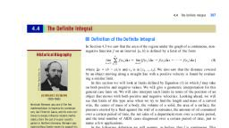
78, , Chapter 1 Limits, , 1.1, , An Intuitive Introduction to Limits, A Real-Life Example, A prototype of a maglev (magnetic levitation train) moves along a straight monorail., To describe the motion of the maglev, we can think of the track as a coordinate line., From data obtained in a test run, engineers have determined that the maglev’s displacement (directed distance) measured in feet from the origin at time t (in seconds) is given, by, s  f(t)  4t 2, , 0  t  30, , (1), , where f is called the position function of the maglev. The position of the maglev at, time t  0, 1, 2, 3, p , 30, measured in feet from its initial position, is, f(0)  0,, , f(1)  4,, , f(2)  16,, , f(3)  36,, , p,, , f(30)  3600, , (See Figure 1.), , FIGURE 1, A maglev moving along an, elevated monorail track, , 0, , 4, , 16, , 36, , 3600, , s (ft), , It appears that the maglev is accelerating over the time interval [0, 30] and, therefore, that its velocity varies over time. This raises the following question: Can we find, the velocity of the maglev at any time in the interval (0, 30) using only Equation (1)?, To be more specific, can we find the velocity of the maglev when, say, t  2?, For a start, let’s see what quantities we can compute. We can certainly compute the, position of the maglev for some selected values of t by using Equation (1), as we did, earlier. Using these values of f, we can then compute the average velocity of the maglev, over any interval of time. For example, to compute the average velocity of the train, over the time interval [2, 4], we first compute the displacement of the train over that, interval, f(4)  f(2), and then divide this quantity by the time elapsed. Thus,, displacement, f(4)  f(2), 4(4)2  4(2)2, 64  16, , , ,  24, time elapsed, 42, 2, 2, or 24 ft/sec. Although this is not quite the velocity of the maglev at t  2, it does provide us with an approximation of its velocity at that time., Can we do better? Intuitively, the smaller the time interval we pick (with t  2 as, the left endpoint), the more closely the average velocity over that time interval will, approximate the actual velocity of the maglev at t  2.*, Now let’s describe this process in general terms. Let t  2. Then the average velocity of the maglev over the time interval [2, t] is given by, √av , , f(t)  f(2), 4t 2  4(2)2, 4(t 2  4), , , t2, t2, t2, , *Actually, any interval containing t  2 will do., , (2)

Page 27 :
1.1, , An Intuitive Introduction to Limits, , 79, , By choosing the values of t closer and closer to 2, we obtain a sequence of numbers, that gives the average velocities of the maglev over smaller and smaller time intervals., As we observed earlier, this sequence of numbers should approach the instantaneous, velocity of the train at t  2., Let’s try some sample calculations. Using Equation (2) and taking the sequence, t  2.5, 2.1, 2.01, 2.001, and 2.0001, which approaches 2, we find, 4(2.52  4),  18 ft/sec, 2.5  2, 4(2.12  4), The average velocity over [2, 2.1] is,  16.4 ft/sec, 2.1  2, The average velocity over [2, 2.5] is, , and so forth. These results are summarized in Table 1. From the table we see that the, average velocity of the maglev seems to approach the number 16 as it is computed over, smaller and smaller time intervals. These computations suggest that the instantaneous, velocity of the train at t  2 is 16 ft/sec., TABLE 1 The average velocity of the maglev, t, av, , over [2, t], , 2.5, , 2.1, , 2.01, , 2.001, , 2.0001, , 18, , 16.4, , 16.04, , 16.004, , 16.0004, , Note We cannot obtain the instantaneous velocity for the maglev at t  2 by substituting t  2 into Equation (2) because this value of t is not in the domain of the average velocity function., , Intuitive Definition of a Limit, Consider the function t defined by, t(t) , , 4(t 2  4), t2, , which gives the average velocity of the maglev (see Equation (2)). Suppose that we, are required to determine the value that t(t) approaches as t approaches the (fixed), number 2. If we take a sequence of values of t approaching 2 from the right-hand side,, as we did earlier, we see that t(t) approaches the number 16. Similarly, if we take a, sequence of values of t approaching 2 from the left, such as t  1.5, 1.9, 1.99, 1.999,, and 1.9999, we obtain the results in Table 2., TABLE 2 The values of t as t approaches 2, from the left, t, , 1.5, , 1.9, , 1.99, , 1.999, , 1.9999, , g(t), , 14, , 15.6, , 15.96, , 15.996, , 15.9996, , Observe that t(t) approaches the number 16 as t approaches 2—this time from the, left-hand side. In other words, as t approaches 2 from either side of 2, t(t) approaches, 16. In this situation we say that the limit of t(t) as t approaches 2 is 16, written, lim t(t)  lim, t→2, , t→2, , 4(t 2  4),  16, t2

Page 28 :
80, , Chapter 1 Limits, , The graph of the function t, shown in Figure 2, confirms this observation., y, 20, , y  g(t), , 16, f(t), 12, 8, 4, 2, , FIGURE 2, As t approaches 2, t(t) approaches 16., , 1, , 0, , 1 t, , 2, , 3, , 4, , t, , Note Observe that the number 2 does not lie in the domain of t. (For this reason the, point (2, 16) is not on the graph of t, and we indicate this by an open circle on the, graph.) Notice, too, that the existence or nonexistence of t(t) at t  2 plays no role in, our computation of the limit., , DEFINITION Limit of a Function at a Number, Let f be a function defined on an open interval containing a, with the possible, exception of a itself. Then the limit of f(x) as x approaches a is the number L,, written, lim f(x)  L, , (3), , x→a, , if f(x) can be made as close to L as we please by taking x to be sufficiently close, to a., , EXAMPLE 1 Use the graph of the function f shown in Figure 3 to find the given limit,, if it exists., a. lim f(x), x→1, , b. lim f(x), x→3, , c. lim f(x), x→5, , d. lim f(x), , e. lim f(x), , x→7, , x→10, , y, 5, 4, 3, 2, 1, , FIGURE 3, The graph of the function f, , 0, , 1 2 3 4 5 6 7 8, , 9 10, , 15, , x, , Solution, a. The values of f can be made as close to 2 as we please by taking x to be sufficiently close to 1. So lim x→1 f(x)  2., b. The values of f can be made as close to 3 as we please by taking x to be sufficiently close to 3. So lim x→3 f(x)  3. Observe that f(3)  1, but this has no, bearing on the answer.

Page 29 :
1.1, , An Intuitive Introduction to Limits, , 81, , c. No matter how close x is to 5, there are values of f, corresponding to values of, x smaller than 5, that are close to 1; and there are values of f, corresponding to, values of x greater than 5, that are close to 4. In other words, there is no unique, number that f(x) approaches as x approaches 5. Therefore, lim x→5 f(x) does not, exist. Observe that f(5)  1, but, again, this has no bearing on the existence or, nonexistence of the limit., d. No matter how close x is to 7, there are values of f that are close to 2 (corresponding to values of x less than 7) and values of f that are close to 4 (corresponding to values of x greater than 7). So lim x→7 f(x) does not exist. Observe, that x  7 is not in the domain of f, but this does not affect our answer., e. As x approaches 10 from the right, f(x) increases without bound. Therefore, f(x), cannot approach a unique number as x approaches 10, and lim x→10 f(x) does not, exist. Here, f(10)  1, but this fact plays no role in our determination of the, limit., Note Example 1 shows that when we evaluate the limit of a function f as x approaches, a, it is immaterial whether f is defined at a. Furthermore, even if f is defined at a,, the value of f at a, f(a), has no bearing on the existence or the value of the limit in, question., , EXAMPLE 2 Find lim x→2 f(x) if it exists, where f is the piecewise-defined function, f(x)  e, , 4x  8 if x  2, 4, if x  2, , y, y  f(x), , 20, 16, 12, , Solution From the graph of f shown in Figure 4, we see that lim x→2 f(x)  16. If you, compare the function f with the function t discussed earlier (page 80), you will see, that the values of f are identical to the values of t except at x  2 (Figures 2 and 4)., Thus, the limits of f(x) and t(x) as x approaches 2 are equal, as expected. We can see, why the graphs of the two functions coincide everywhere except at x  2 by writing, , 8, , t(x) , , 4, 2 1, , 0, , 1, , 2, , 3, , x, , 4, , FIGURE 4, The graph of f coincides with the graph, of the function t shown in Figure 2,, except at x  2., , , , The Heaviside function H (the unit step func0 if t  0, 1 if t 0, , This function, named after Oliver Heaviside (1850–1925), can be used to describe the, flow of current in a DC electrical circuit that is switched on at time t  0. Show that, lim t→0 H(t) does not exist., , 1, , FIGURE 5, lim t→0 H(t) does not exist., , Assume that x  2., , which is equivalent to the rule defining f when x  2., , H(t)  e, , y, , Use x instead of t., , 4(x  2)(x  2), x2, ,  4(x  2), , EXAMPLE 3 The Heaviside Function, tion) is defined by, , 0, , 4(x 2  4), x2, , t, , Solution The graph of H is shown in Figure 5. You can see from the graph that no, matter how close t is to 0, H(t) takes on the value 1 or 0, depending on whether t is, to the right or to the left of 0. Therefore, H(t) cannot approach a unique number L as, t approaches 0, and we conclude that lim t→0 H(t) does not exist.

Page 30 :
82, , Chapter 1 Limits, , One-Sided Limits, Let’s reexamine the Heaviside function. We have shown that lim t→0 H(t) does not exist,, but what can we say about the behavior of H(t) at values of t that are close to but, greater than 0? If you look at Figure 5 again, it is evident that as t approaches 0 through, positive values (from the right of 0), H(t) approaches 1. In this situation we say that, the right-hand limit of H as t approaches 0 is 1, written, lim H(t)  1, , t→0, , More generally, we have the following:, , DEFINITION Right-Hand Limit of a Function, Let f be a function defined for all values of x close to but greater than a. Then, the right-hand limit of f(x) as x approaches a is equal to L, written, lim f(x)  L, , x→a, , (4), , if f(x) can be made as close to L as we please by taking x to be sufficiently close, to but greater than a., , Note, , Equation (4) is just Equation (3) with the further restriction x  a., , The left-hand limit of a function is defined in a similar manner., , DEFINITION Left-Hand Limit of a Function, Let f be a function defined for all values of x close to but less than a. Then the, left-hand limit of f(x) as x approaches a is equal to L, written, lim f(x)  L, , x→a, , (5), , if f(x) can be made as close to L as we please by taking x to be sufficiently close, to but less than a., y, 3, 2, 1, 0, , 1, , 2, , 3, , 4, , x, , FIGURE 6, The right-hand limit of f(x)  1x  1, as x approaches 1 is 0., , For the function H of Example 3 we have lim t→0 H(t)  0., The right-hand and left-hand limits of a function, lim x→a f(x) and lim x→a f(x) ,, are often referred to as one-sided limits, whereas lim x→a f(x) is called a two-sided, limit., For some functions it makes sense to look only at one-sided limits. Consider, for, example, the function f defined by f(x)  1x  1, whose domain is [1, ⬁). Here it, makes sense to talk only about the right-hand limit of f(x) as x approaches 1. Also,, from Figure 6, we see that lim x→1 f(x)  0.

Page 31 :
1.1, , An Intuitive Introduction to Limits, , 83, , EXAMPLE 4 Let f(x)  24  x 2. Find lim x→2 f(x) and lim x→2 f(x)., , y, , , , 2, , y  4  x2, , , , Solution The graph of f is the upper semicircle shown in Figure 7. From this graph, we see that lim x→2 f(x)  0 and lim x→2 f(x)  0., Theorem 1 gives the connection between one-sided limits and two-sided limits., , 0, , 2, , x, , 2, , FIGURE 7, We can approach 2 only from the, right and 2 only from the left., , THEOREM 1 Relationship Between One-Sided and Two-Sided Limits, Let f be a function defined on an open interval containing a, with the possible, exception of a itself. Then, lim f(x)  L if and only if, , x→a, , lim f(x)  lim f(x)  L, , x→a, , x→a, , (6), , Thus, the (two-sided) limit exists if and only if the one-sided limits exist and are equal., , EXAMPLE 5 Sketch the graph of the function f defined by, 3x, if x  1, f(x)  • 1, if x  1, 2  1x  1 if x  1, , y, 4, 3, , Use your graph to find lim x→1 f(x), lim x→1 f(x), and lim x→1 f(x)., , 2, 1, 3 2 1 0, , Solution, 1, , 2, , 3, , 4, , 5, , FIGURE 8, lim f(x)  lim f(x)  lim f(x)  2, x→1, , x→1, , x→1, , From the graph of f, shown in Figure 8, we see that, lim f(x)  2, , x, , x→1, , and, , lim f(x)  2, , x→1, , Since the one-sided limits are equal, we conclude that lim x→1 f(x)  2. Notice that, f(1)  1, but this has no effect on the value of the limit., , EXAMPLE 6 Let f(x) , , x, , 1, , sin x, . Use your calculator to complete the following table., x, , 0.5, , 0.1, , 0.05, , 0.01, , 0.005, , 0.001, , sin x, x, , Then sketch the graph of f, and use your graph to guess at the value of lim x→0 f(x),, lim x→0 f(x), and lim x→0 f(x)., Solution Using a calculator, we obtain Table 3. (Remember to use radian mode!) The, graph of f is shown in Figure 9. We find, lim f(x)  1,, , x→0, , lim f(x)  1,, , x→0, , and so, , lim f(x)  1, , x→0, , We will prove in Section 1.2 that our guesses here are correct.

Page 32 :
84, , Chapter 1 Limits, , TABLE 3, , 1, 0.5, 0.1, 0.05, 0.01, 0.005, 0.001, , 0.841470985, 0.958851077, 0.998334166, 0.999583385, 0.999983333, 0.999995833, 0.999999833, , EXAMPLE 7 Let f(x) , a. lim f(x), , 1, x2, , 1, , 0, , 1, , 1, , x, , FIGURE 9, sin x, The graph of f(x) , x, , . Evaluate the limit, if it exists., , b. lim f(x), , x→0, , y, , sin x, x, , x, , x→0, , c. lim f(x), x→0, , Solution Some values of the function are listed in Table 4, and the graph of f is shown, in Figure 10., , Historical Biography, y, , Bettmann/Corbis, , TABLE 4, x, , JOHN WALLIS, (1616–1703), The first mathematician to use the symbol, ⬁ to indicate infinity, John Wallis contributed to the earliest forms, notations,, and terms of calculus and other areas of, mathematics. Born November 23, 1616, in, the borough of Ashford, in Kent, England,, Wallis attended boarding school as a child,, and his exceptional mathematical ability, was evident at an early age. He mastered, arithmetic in two weeks and was able to, solve a problem such as the square root of, a 53-digit number to 17 places without, notation. Considered to be the most influential British mathematician before Isaac, Newton (page 179), Wallis published his, first major work, Arithmetica Infinitorum,, in 1656. It became a standard reference, and is still recognized as a monumental, text in British mathematics., , 1, 0.5, 0.1, 0.05, 0.01, 0.001, , f(x) , , 1, x2, 1, 4, 100, 400, 10,000, 1,000,000, , 1, x2, , 1, 1, , 0, , 1, , x, , FIGURE 10, As x → 0 from the left (or from the, right), f(x) increases without bound., , a. As x approaches 0 from the left, f(x) increases without bound and does not, approach a unique number. Therefore, lim x→0 f(x) does not exist., b. As x approaches 0 from the right, f(x) increases without bound and does not, approach a unique number. Therefore, lim x→0 f(x) does not exist., c. From the results of parts (a) and (b) we conclude that lim x→0 f(x) does not exist., , Note Even though the limit lim x→0 f(x) does not exist, we write lim x→0 (1>x 2)  ⬁, to indicate that f(x) increases without bound as x approaches 0. We will study “infinite, limits” in Section 3.5.

Page 33 :
1.1, , An Intuitive Introduction to Limits, , 85, , Using Graphing Utilities to Evaluate Limits, In Example 6 we employed both a numerical and a graphical approach to help us conjecture that, sin x, 1, lim, x→0 x, Either or both of these approaches can often be used to estimate the limit of a function as x approaches a specified value. But there are pitfalls in using graphing utilities,, as the following examples show., , EXAMPLE 8 Use a graphing utility to find, lim, , x→0, , 1x  4  2, x, , Solution We first investigate the problem numerically by constructing a table of values of f(x)  ( 1x  4  2)>x corresponding to values of x that approach 0 from either, side of 0. Table 5a shows the values of f for x close to but to the left of 0, and Table, 5b shows the values of f for x close to but to the right of 0., If you look at f evaluated at the first nine values of x shown in each column, we, are tempted to conclude that the required limit is 14. But how do we reconcile this result, with the last two values of f in each column? Upon reflection we see that this discrepancy can be attributed to a phenomenon known as loss of significance., TABLE 5 Values of f for x close to 0, x, , 1x ⴙ 4 ⴚ 2, x, , 0.001, 0.0001, 105, 106, 107, 108, 109, 1010, 1011, 1012, 1013, , 0.250015627, 0.250001562, 0.25000016, 0.25, 0.25, 0.25, 0.25, 0.25, 0.25, 0.3, 0, , (a) x approaches 0 from the left., , x, 0.001, 0.0001, 105, 106, 107, 108, 109, 1010, 1011, 1012, 1013, , 1x ⴙ 4 ⴚ 2, x, 0.249984377, 0.249998438, 0.24999984, 0.25, 0.25, 0.25, 0.25, 0.25, 0.25, 0.2, 0, , (b) x approaches 0 from the right., , When x is very small, the computed values of 1x  4 are very close to 2. For, x  1013 or x  1013 (and values that are smaller in absolute value) the calculator rounds off the value of 1x  4 to 2 and gives the value of f(x) as 0. Figures 11a–b show the graphs of f using the viewing windows [2, 2] [0.2, 0.3] and, [103, 103] [0.2, 0.3], respectively. Both these graphs reinforce the earlier, observation that the required limit is 14 . The graph of f using the viewing window, [1011, 1011] [0.24995, 0.25005], shown in Figure 11c, proves to be of no help, because of the problem with loss of significance stated earlier.

Page 34 :
86, , Chapter 1 Limits, , .30, , .30, , .25005, , 1011, , 2, (a) [2, 2], , .001, , 2, , .20, , .001, , .20, , (b) [103, 103], , [0.2, 0.3], , 1011, , .24995, (c) [1011, 1011], , [0.2, 0.3], , [0.24995, 0.25005], , FIGURE 11, 1x  4  2, The graphs of f(x) , in different viewing windows, x, , Having recognized the source of the difficulty, how can we remedy the situation?, Let’s find another expression for f(x) that does not involve subtracting numbers that, are so close to each other that it results in a loss of significance. Rationalizing the, numerator, we obtain, f(x) , , 1x  4  2 1x  4  2, 1x  4  2, , ⴢ, x, x, 1x  4  2, , , (x  4)  4, x( 1x  4  2), , , , 1, 1x  4  2, , (a  b)(a  b)  a 2  b 2, , x0, , Observe that the use of the last expression avoids the pitfalls that we encountered with, the original expression. We leave it as an exercise to show that both a numerical analysis and a graphical analysis of, lim, , x→0, , 1, 1x  4  2, , suggest that a good guess for, lim, , x→0, , 1x  4  2, 1,  lim, x, x→0 1x  4  2, , 1, 4,, , is a result that can be proved analytically using the techniques to be developed in, the next section., 1, x, , EXAMPLE 9 Find lim sin ., x→0, , 1.2, , 1, , 1, , 1.2, , FIGURE 12, The graph of f(x)  sin(1>x) in the, viewing window [1, 1] [1.2, 1.2], , Solution Let f(x)  sin(1>x). The graph of f using the viewing window, [1, 1] [1.2, 1.2] does not seem to be of any help to us in finding the required, limit (see Figure 12). To obtain a more accurate graph of f(x)  sin(1>x), note that the, sine function is bounded by 1 and 1. Thus, the graph of f lies between the horizontal lines y  1 and y  1. Next, observe that the sine function has period 2p. Since, 1>x increases without bound (decreases without bound) as x approaches 0 from the, right (from the left), we see that sin(1>x) undergoes more and more cycles as x, approaches 0. Thus, the graph of f(x)  sin(1>x) oscillates between 1 and 1, as shown, in Figure 13. Therefore, it seems reasonable to conjecture that the limit does not exist., Indeed, we can demonstrate this conclusion by constructing Table 6.

Page 35 :
1.1, , 1, , y, , 87, , TABLE 6, x, , 1 x, , 0, , 1, , An Intuitive Introduction to Limits, , 1, , sin, , 1, x, , 2, p, , 2, 3p, , 2, 5p, , 2, 7p, , 2, 9p, , 2, 11p, , p, , 1, , 1, , 1, , 1, , 1, , 1, , p, , Note that the values of x approach 0 from the right. From the table we see that no, matter how close x is to 0 (from the right), there are values of f corresponding to these, values of x that are equal to 1 or 1. Therefore, f(x) cannot approach any fixed number as x approaches 0. A similar result is true if the values of x approach 0 from the, left. This shows that, , FIGURE 13, The graph of f(x)  sin(1>x), , lim sin, , x→0, , 1, x, , does not exist., , 1.1, , CONCEPT QUESTIONS, , 1. Explain what is meant by the statement lim x→2 f(x)  3., 2. a. If lim x→3 f(x)  5, what can you say about f(3)?, Explain., b. If f(2)  6, what can you say about lim x→2 f(x)?, Explain., , 1.1, , 3. Explain what is meant by the statement lim x→3 f(x)  2., 4. Suppose lim x→1 f(x)  3 and lim x→1 f(x)  4., a. What can you say about lim x→1 f(x)? Explain., b. What can you say about f(1)? Explain., , EXERCISES, , In Exercises 1–6, use the graph of the function f to find each, limit., 1., , 2., , y, , 3., , y, , 4, , y, 3, , 3, , 4., , y, , 3, , 3, , 2, , 2, , 1, , 1, 1, 3 2 1 0, 1, , 1, 1, , 2, , 3, , x, , 321 0, 1, , 2, , 1 2 3 4, , x, , 2, , 4321 0, , a. lim f(x), , b. lim f(x), , b. lim f(x), , c. lim f(x), , c. lim f(x), , x→2, x→2, x→2, , x→2, x→2, x→2, , V Videos for selected exercises are available online at www.academic.cengage.com/login., , x, , 1, , 0, , 1, , a. lim f(x), , a. lim f(x), , b. lim f(x), , b. lim f(x), , c. lim f(x), , c. lim f(x), , x→1, x→1, , a. lim f(x), , 1 2 3 4, , x→1, , x→3, x→3, x→3, , 2, , 3, , x

Page 36 :
88, , Chapter 1 Limits, , 5., , lim f(x)  1, , b. lim f(x)  f(0), , y, , a., , 2, , c. lim f(x)  2, , d. lim f(x)  3, , e. lim f(x) does not exist, , f. lim f(x)  3, , x→3, , x→0, , x→2, , x→2, , x→3, , 0, , 3 2, , In Exercises 9–16, complete the table by computing f(x) at the, given values of x, accurate to five decimal places. Use the results, to guess at the indicated limit, if it exists., , x, , 1 2 3, , 2, , 9. lim, a., , lim f(x), , 6., , lim f(x), , b., , x→1, , x→5, , x→1, , c. lim f(x), , x→1, , x1, x  3x  2, 2, , x→1, , y, , x, , 3, , 0.9, , 0.99, , 0.999, , 1.001, , 1.01, , 1.1, , 0.999, , 1.001, , 1.01, , 1.1, , 1.999, , 2.001, , 2.01, , 2.1, , f(x), , 2, 1, 1 0, , 1, 1, , 2, , 10. lim, , x, , 3, , x→1, , 2, , x, , 3, , a. lim f(x), , b. lim f(x), , x→0, , x x2, 0.9, , 0.99, , f(x), , c. lim f(x), , x→0, , x1, 2, , x→0, , 7. Use the graph of the function f to determine whether each, statement is true or false. Explain., , 11. lim, , x→2, , 1x  2  2, x2, , y, , x, , 4, , 1.9, , 1.99, , f(x), y  f(x), , 3, 2, , 12. lim, , x→0, , 1, 3, , a., , 2, , 1, , 0, , 1, , 2, , lim f(x)  2, , 3, , 4, , 5, , 6, , x, , 0.1, , x, , 0.01, , 0.001, , 0.001, , 0.01, , 0.1, , f(x), , b. lim f(x)  2, , x→3, , 13  x  13  x, x, , x→0, , c. lim f(x)  1, , d. lim f(x)  3, , e. lim f(x) does not exist, , f. lim f(x)  2, , x→2, , 1, 1, , 2, 12  x, 13. lim, x→2, x2, , x→4, , x→4, , x→4, , 8. Use the graph of the function f to determine whether each, statement is true or false. Explain., , x, , 1.9, , 1.99, , 1.999, , 2.001, , 2.01, , 2.1, , 2.999, , 3.001, , 3.01, , 3.1, , y, , f(x), y  f(x), , 3, 2, , 14. lim, , x→3, , 3 1x  1  2x, x(x  3), , 1, 3, , 2, , 1, , 0, , 1, , 2, , 3, , 4, , 5, , x, , x, f(x), , 2.9, , 2.99

Page 37 :
1.1, , 15. lim, , x→0, , An Intuitive Introduction to Limits, , 89, , x, sin x, 29. Let, 0.1, , x, , 0.01, , 0.001, , 0.001, , 0.01, , 0.1, , f(x)  •, , f(x), , 16. lim, , x→0, , 0.1, , 0.01, , if x  0, , 1, sin, x, , if x  0, , y, , (x  1) cos x  1, (x  1) sin x, , x, , 0, , 1, , 0.001, , 0.001, , 0.01, , 0.1, , x, , 0, , f(x), 1, , In Exercises 17–22, sketch the graph of the function f and evaluate (a) lim x→a f(x), (b) lim x→a f(x), and (c) lim x→a f(x) for the, given value of a., 17. f(x)  e, , x1, if x  3, ;, 2x  8 if x  3, , 2x  4 if x  4, 18. f(x)  e, ;, x  2 if x 4, , a3, , 30. Let, a4, , x 2  4 if x  0, 19. f(x)  e, ;, 2, if x  0, 20. f(x)  e, , x  1 if x  0, ;, 1, if x  0, , lim Œ xœ, , x→1, , 27. lim Œ xœ, x→3.1, , if x  0, , 1, x sin, x, , if x  0, , y  x, , a0, , yx, , a1, , x, , a1, , The symbol Œ œ denotes the greatest integer function defined by, Œ x œ  the greatest integer n such that n  x. For example,, Œ 2.8œ  2, and Œ 2.7œ  3. In Exercises 23–28, use the graph, of the function to find the indicated limit, if it exists., , 25., , 0, , y, , 2, , 2x  4 if x  1, 22. f(x)  • 4, if x  1;, if x  1, x2  1, , x→3, , f(x)  •, , a0, , x, if x  1, 21. f(x)  • 2, if x  1;, x  2 if x  1, , 23. lim Œ xœ, , (As x approaches 0 from the right, y oscillates more and, more.) Use the figure and construct a table of values to, guess at lim x→0 f(x), lim x→0 f(x), and lim x→0 f(x). Justify, your answer., , 24. lim Œ x œ, x→3, , 26. lim Œ x œ, , Use the figure, and construct a table of values to guess at, lim x→0 f(x), lim x→0 f(x), and lim x→0 f(x). Justify your, answer., 31. Let, 1, x, f(x)  d, sin x, 0, , if x  0, if 0  x  p, if x p, , x→1, , 28. lim Œ 2x œ, x→2.4, , a. Sketch the graph of f., b. Find all values of x in the domain of f at which the limit, of f exists., c. Find all values of x in the domain of f at which the lefthand limit of f exists., d. Find all values of x in the domain of f at which the righthand limit of f exists.

Page 38 :
90, , Chapter 1 Limits, , 32. Let, , if x  0, if 0  x  p2, if x p2, , x 2, f(x)  • tan x, 1, , a. Sketch the graph of f., b. Find all values of x in the domain of f at which the limit, of f exists., c. Find all values of x in the domain of f at which the lefthand limit of f exists., d. Find all values of x in the domain of f at which the righthand limit of f exists., , 35. Let f(h)  (1  h)1>h, and assume that lim h→0 (1  h)1>h, exists. (We will establish this in Chapter 6.) Find its value, to four decimal places of accuracy by computing f(h) for, h  0.1, 0.01, 0.001, 0.0001, 0.00001, 0.000001, and, 0.0000001., 36. Let f(u)  (tan u  u)>u3. By computing f(u) for u  0.1,, 0.01, and 0.001, accurate to five decimal places, guess at, lim u→0 (tan u  u)>u3., In Exercises 37–42, plot the graph of f. Then use the graph to, guess at the specified limit (if it exists)., 37. f(x) , , 2x 2  x  6, ;, x2, , x→2, , 38. f(x) , , x3, ;, 1x  1  2, , x→3, , where c is a constant and t 0 0. Show that if c  0, then, lim t→t0 Hc(t  t 0) does not exist., , 39. f(x) , , x 3  x 2  3x  1, ;, 冟x  1冟, , 34. The Square-Wave Function The square-wave function f can be, expressed in terms of the Heaviside function (Exercise 33), as follows:, , 40. f(x) , , tan x, ;, x, , 33. The Heaviside Function A generalization of the unit step function or Heaviside function H of Example 3 is the function, Hc defined by, 0 if t  t 0, Hc(t  t 0)  e, c if t t 0, , f(t)  Hk(t)  Hk(t  k)  Hk(t  2k),  Hk(t  3k)  Hk(t  4k)  p, , 41. f(x) , 42. f(x) , , Referring to the following figure, show that lim t→nk f(t) does, not exist for n  1, 2, 3, p ., y, , sin 2x, ;, tan 4x, , lim f(x), lim f(x), , x→1, , lim f(x), , x→0, , cos x  1, x2, , lim f(x), , ;, , lim f(x), , x→0, , lim f(x), , x→0, , In Exercises 43–46, determine whether the statement is true or, false. If it is true, explain why. If it is false, explain why or give, an example that shows it is false., 43. If lim x→a f(x)  c, then f(a)  c., , k, , 44. If f is defined at a, then lim x→a f(x) exists., 45. If lim x→a f(x)  lim x→a t(x), then f(a)  t(a)., , 0, , 1.2, , k, , 2k, , 3k, , 4k, , 5k, , t, , 46. If both lim x→a f(x) and lim x→a f(x) exist, then lim x→a f(x), exists., , Techniques for Finding Limits, Computing Limits Using the Laws of Limits, In Section 1.1 we used tables of functional values and graphs of functions to help us, guess at the limit of a function, if it exists. This approach, however, is useful only in, suggesting whether the limit exists and what its value might be for simple functions., In practice, the limit of a function is evaluated by using the laws of limits that we now, introduce., , LAW 1 Limit of a Constant Function f(x) ⴝ c, If c is a real number, then, lim c  c, , x→a

Page 39 :
1.2, , Techniques for Finding Limits, , 91, , You can see this intuitively by studying the graph of the constant function f(x)  c, shown in Figure 1. You will be asked to prove this law in Exercise 15, Section 1.3., , y, yc, , EXAMPLE 1 lim x→2 5  5, lim x→1 3  3, and lim x→0 2p  2p., 0, , x, , a, , LAW 2 Limit of the Identity Function f(x) ⴝ x, , FIGURE 1, For the constant function f(x)  c,, lim x→a f(x)  c., y, , lim x  a, , x→a, , yx, , Again, you can see this intuitively by examining the graph of the identity function, f(x)  x. (See Figure 2.) You will also be asked to prove this law in Exercise 16, Section 1.3., , a, , EXAMPLE 2 lim x→4 x  4, lim x→0 x  0, and lim x→p x  p., 0, , a, , FIGURE 2, If f is the identity function f(x)  x,, then lim x→a f(x)  a., , x, , The following limit laws allow us to find the limits of functions algebraically., , LIMIT LAWS, If lim x→a f(x)  L and lim x→a t(x)  M, then, , LAW 3 Sum Law, lim[ f(x), , x→a, , t(x)]  L, , M, , LAW 4 Product Law, lim[ f(x)t(x)]  LM, , x→a, , LAW 5 Constant Multiple Law, lim[cf(x)]  cL, for every c, , x→a, , LAW 6 Quotient Law, f(x), L,  , provided that M  0, x→a t(x), M, lim, , LAW 7 Root Law, n, , n, , lim 1f(x)  1L, provided that n is a positive integer,, and L  0 if n is even, , x→a, , In words, these laws say the following:, 3. The limit of the sum (difference) of two functions is the sum (difference) of, their limits., 4. The limit of the product of two functions is the product of their limits., 5. The limit of a constant times a function is the constant times the limit of the, function.

Page 40 :
92, , Chapter 1 Limits, , 6. The limit of a quotient of two functions is the quotient of their limits, provided, that the limit of the denominator is not zero., 7. The limit of the nth root of a function is the nth root of the limit of the function,, provided that n is a positive integer and L  0 if n is even., (We will prove the Sum Law in Section 1.3. The other laws are proved in Appendix B.), Although the Sum Law and the Product Law are stated for two functions, they are, also valid for any finite number of functions. For example, if, lim f1(x)  L 1,, , x→a, , lim f2(x)  L 2,, , x→a, , p,, , lim fn(x)  L n, , x→a, , then, lim[ f1(x)  f2(x)  p  fn (x)]  L 1  L 2  p  L n, , x→a, , and, lim[f1(x)f2(x) p fn (x)]  L 1L 2 p L n, , (1), , x→a, , If we take f1(x)  f2(x)  p  fn (x)  f(x), then Equation (1) gives the following, result for powers of f., , LAW 8 If n is a positive integer and lim x→a f(x)  L, then lim x→a[ f(x)]n  Ln., Next, if we take f(x)  x, then Equation (1) and Law 8 give the following result., , LAW 9 lim x→a x n  a n, where n is a positive integer., , EXAMPLE 3 Find lim x→2(2x 3  4x 2  3)., Solution, lim (2x 3  4x 2  3)  lim 2x 3  lim 4x 2  lim 3, , x→2, , x→2, , x→2, , Law 3, , x→2, ,  2 lim x 3  4 lim x 2  lim 3, , Law 5, ,  2(2)3  4(2)2  3, , Law 9, , x→2, , x→2, , x→2, , 3, , Limits of Polynomial and Rational Functions, The method of solution that we used in Example 3 can be used to prove the following., , LAW 10 Limits of Polynomial Functions, If p(x)  anx n  an1x n1  p  a0 is a polynomial function, then, lim p(x)  p(a), , x→a

Page 41 :
1.2, , Techniques for Finding Limits, , 93, , Thus, the limit of a polynomial function as x approaches a is equal to the value of, the function at a., , PROOF Applying the (generalized) sum law and the constant multiple law repeatedly,, we find, lim p(x)  lim (anx n  an1x n1  p  a0), , x→a, , x→a, ,  an(lim x n)  an1(lim x n1)  p  lim a0, x→a, , x→a, , x→a, , Next, using Laws 1, 2, and 9, we obtain, lim p(x)  ana n  an1a n1  p  a0  p(a), , x→a, , In light of this, we could have solved the problem posed in Example 3 as follows:, lim (2x 3  4x 2  3)  2(2)3  4(2)2  3  3, , x→2, , EXAMPLE 4 Find lim x→1(3x 2  2x  1)5., Solution, lim (3x 2  2x  1)5  [ lim (3x 2  2x  1)]5, , x→1, , Law 8, , x→1, ,  [3(1)2  2(1)  1]5, , Law 10, ,  25  32, The following result follows from the Quotient Law for limits and Law 10., , LAW 11 Limits of Rational Functions, If f is a rational function defined by f(x)  P(x)>Q(x), where P(x) and Q(x) are, polynomial functions and Q(a)  0, then, lim f(x)  f(a) , , x→a, , P(a), Q(a), , Thus, the limit of a rational function as x approaches a is equal to the value of the, function at a provided the denominator is not zero at a., , PROOF Since P and Q are polynomial functions, we know from Law 10 that, lim P(x)  P(a), , x→a, , and, , lim Q(x)  Q(a), , x→a, , Since Q(a)  0, we can apply the Quotient Law to conclude that, lim P(x), P(x), P(a), x→a, , ,  f(a), x→a Q(x), lim Q(x), Q(a), , lim f(x)  lim, , x→a, , x→a

Page 42 :
94, , Chapter 1 Limits, , 4x 2  3x  1, ., x→3, 2x  4, , EXAMPLE 5 Find lim, Solution, , Using Law 11, we obtain, 4(3)2  3(3)  1, 4x 2  3x  1, 28, , ,  14, x→3, 2x  4, 2(3)  4, 2, lim, , EXAMPLE 6 Find lim, , x→1, , 3 2x  14, ., B x2  1, , Solution, lim, , x→1, , 2x  14, 3 2x  14,  3 lim 2, B x2  1, B x→1 x  1, , , 3, , 2(1)  14, , B 12  1, , Law 7, , Law 11, , 3,  1, 82, , Lest you think that we can always find the limit of a function by substitution, consider the following example., , x2  4, ., x→2 x  2, , EXAMPLE 7 Find lim, , Solution Because the denominator of the rational expression is 0 at x  2, we cannot find the limit by direct substitution. However, by factoring the numerator, we obtain, (x  2)(x  2), x2  4, , x2, x2, so if x  2, we can cancel the common factors. Thus,, x2  4, x2, x2, , x2, , In other words, the values of the function f defined by f(x)  (x 2  4)>(x  2) coincide with the values of the function t defined by t(x)  x  2 for all values of x except, x  2. Since the limit of f(x) as x approaches 2 depends only on the values of x other, than 2, we can find the required limit by evaluating the limit of t(x) as x approaches, 2 instead. Thus,, x2  4,  lim (x  2)  2  2  4, x→2 x  2, x→2, lim, , In certain instances the technique that we used in Example 7 can be applied to find, the limit of a quotient in which both the numerator and denominator of the quotient, approach 0 as x approaches a. The trick here is to use the appropriate algebraic manipulations that will enable us to replace the original function by one that is identical to, that function except perhaps at a. The limit is then found by evaluating this function, at a.

Page 43 :
1.2, , Techniques for Finding Limits, , 95, , Notes, 1. If the numerator does not approach 0 but the denominator does, then the limit of, the quotient does not exist. (See Example 7 in Section 1.1.), 2. A function whose limit at a can be found by evaluating it at a is said to be continuous at a. (We will study continuous functions in Section 1.4.), , EXAMPLE 8 Find lim, , x 2  2x  3, , x→3, , x 2  4x  3, , ., , Solution Notice that both the numerator and the denominator of the quotient approach, 0 as x approaches 3, so Law 6 is not applicable. Instead, we proceed as follows:, lim, , x→3, , x 2  2x  3, x  4x  3, 2, ,  lim, , x→3, , (x  3)(x  1), (x  3)(x  1), , x1, x→3 x  1, ,  lim, , , EXAMPLE 9 Find lim, , x→0, , x  3, , 3  1, 2, 3  1, , 11  x  1, ., x, , Solution Both the numerator and the denominator of the quotient approach 0 as x, approaches 0, so we cannot evaluate the limit using Law 6. Let’s rationalize the numerator of the quotient by multiplying both the numerator and the denominator by, 11  x  1. Thus,, lim, , x→0, , 11  x  1, 11  x  1 11  x  1,  lim, ⴢ, x, x, x→0, 11  x  1,  lim, , x→0, , ( 11  x  1)( 11  x  1), x( 11  x  1), , 1x1, x→0 x( 11  x  1), ,  lim,  lim, , x→0, , 1, 1, , 2, 11  x  1, , Difference of two squares, , x0, , All of the limit laws stated for two-sided limits in this section also hold true for, one-sided limits., , EXAMPLE 10 Let, f(x)  e, Find lim x→2 f(x) if it exists., , x  3, if x  2, 1x  2  1 if x 2

Page 44 :
96, , Chapter 1 Limits, , Solution The function f is defined piecewise. For x 2 the rule for f is, f(x)  1x  2  1. Letting x approach 2 from the right, we obtain, lim ( 1x  2  1)  lim 1x  2  lim 1, , y, , x→2, , x→2, , 4, , Sum Law, , x→2, , 011, y  f(x), , 3, , For x  2, f(x)  x  3, and, lim (x  3)  lim(x)  lim 3, , 2, , x→2, , x→2, , Sum Law, , x→2, ,  2  3  1, , 1, 0, , 1, , 2, , 3, , 4, , The right-hand and left-hand limits are equal. Therefore, the limit exists and, , x, , 5, , lim f(x)  1, , x→2, , FIGURE 3, lim x→2 f(x)  lim x→2 f(x)  1, so, lim x→2 f(x)  1., , The graph of f is shown in Figure 3., The next example involves the greatest integer function defined by f(x)  Œxœ ,, where Œ xœ is the greatest integer n such that n  x. For example, Œ3œ  3, Œ2.4 œ  2,, Œpœ  3, Œ4.6 œ  5, Œ 12 œ  2, and so on. As an aid to finding the value of, the greatest integer function, think of “rounding down.”, , EXAMPLE 11 Show that lim Œxœ does not exist., , y, , x→2, , 2, , Solution The graph of the greatest integer function is shown in Figure 4. Observe that, if 2  x  3, then Œx œ  2, and therefore,, , y  “x‘, 1, 2 1, , 0, , 1, , 2, , 3, , 4, , x, , lim Œxœ  lim2  2, , x→2, , Next, observe that if 1  x  2, then Œxœ  1, so, , lim Œxœ  lim 1  1, , 2, , FIGURE 4, The graph of y  Œ xœ, , x→2, , x→2, , x→2, , Since these one-sided limits are not equal, we conclude by Theorem 1, Section 1.1,, that lim x→2 Œxœ does not exist., , Limits of Trigonometric Functions, So far, we have dealt with limits involving algebraic functions. The following theorem, tells us that if a is a number in the domain of a trigonometric function, then the limit, of that function as x approaches a can be found by substitution., , THEOREM 1 Limits of Trigonometric Functions, Let a be a number in the domain of the given trigonometric function. Then, a. lim sin x  sin a, , b. lim cos x  cos a, , c. lim tan x  tan a, , d. lim cot x  cot a, , e. lim sec x  sec a, , f. lim csc x  csc a, , x→a, x→a, x→a, , x→a, x→a, x→a, , The proofs of Theorem 1a and Theorem 1b are sketched in Exercises 97 and 98., The proofs of the other parts follow from Theorems 1a and 1b and the limit laws.

Page 45 :
1.2, , Techniques for Finding Limits, , 97, , EXAMPLE 12 Find, b. lim (2x 2  cot x), , a. lim x sin x, x→p>2, , x→p>4, , Solution, p, p, p, a. lim x sin x  Q lim xRQ lim sin xR  sin , x→p>2, x→p>2, x→p>2, 2, 2, 2, b. lim (2x 2  cot x)  lim 2x 2  lim cot x, x→p>4, , x→p>4, , x→p>4, , 2, , p, p,  2 a b  cot, 4, 4, , , p2, p2  8, 1, 8, 8, , The Squeeze Theorem, The techniques that we have developed so far do not work in all situations. For example, they cannot be used to find, lim x 2 sin, , x→0, , 1, x, , For limits such as this we use the Squeeze Theorem., , THEOREM 2 The Squeeze Theorem, Suppose that f(x)  t(x)  h(x) for all x in an open interval containing a, except, possibly at a, and, lim f(x)  L  lim h(x), , x→a, , x→a, , Then, lim t(x)  L, , x→a, , The Squeeze Theorem says that if t(x) is squeezed between f(x) and h(x) near a, and both f(x) and h(x) approach L as x approaches a, then t(x) must approach L as, well (see Figure 5). A proof of this theorem is given in Appendix B., y, y  h(x), , y  g(x), y  f(x), , L, , FIGURE 5, An illustration of the Squeeze Theorem, , 0, , a, , x

Page 46 :
98, , Chapter 1 Limits, , 1, x, , EXAMPLE 13 Find lim x 2 sin ., x→0, , Solution, , Since 1  sin t  1 for every real number t, we have, , y, 0.3, , 1  sin, , 1, 1, x, , for every x  0. Therefore,, y, , y, , x2, , 0, , 0.6, , sin 1x, , x2, , x, , 0.6, , x0, , Let f(x)  x 2, t(x)  x 2 sin(1>x) , and h(x)  x 2. Then f(x)  t(x)  h(x). Since, lim f(x)  lim (x 2)  0, , y  x2, , x→0, , lim h(x)  lim x 2  0, , and, , x→0, , x→0, , x→0, , the Squeeze Theorem implies that, , 0.3, , lim t(x)  lim x 2 sin, , FIGURE 6, lim t(x)  lim x 2 sin, , x→0, , 1,  x2, x, , x 2  x 2 sin, , x→0, , x→0, , 1, 0, x, , x→0, , 1, 0, x, , (See Figure 6.), The property of limits given in Theorem 3 will be used later. (Its proof is given in, Appendix B.), , THEOREM 3, Suppose that f(x)  t(x) for all x in an open interval containing a, except possibly at a, and, lim f(x)  L, , lim t(x)  M, , and, , x→a, , x→a, , Then, LM, The Squeeze Theorem can be used to prove the following important result, which, will be needed in our work later on., , THEOREM 4, lim, u→0, , C, B, , sin u, 1, u, , PROOF First, suppose that 0  u  p2 . Figure 7 shows a sector of a circle of radius 1., From the figure we see that, Area of 䉭OAB , , sin ¨, , tan ¨, , ¨, O, , FIGURE 7, , 1, , A, , 1, 1, (1)(sin u)  sin u, 2, 2, , Area of sector OAB , Area of 䉭OAC , , 1, 1, (1)2u  u, 2, 2, , 1, 1, (1)(tan u)  tan u, 2, 2, , 1, base ⴢ height, 2, 1 2, r u, 2, 1, base ⴢ height, 2

Page 47 :
1.2, , Techniques for Finding Limits, , 99, , Since 0  area of 䉭OAB  area of sector OAB  area of 䉭OAC, we have, 0, , 1, 1, 1, sin u  u  tan u, 2, 2, 2, , Multiplying through by 2>(sin u) and keeping in mind that sin u  0 and cos u  0, for 0  u  p2 , we obtain, 1, , u, 1, , sin u, cos u, , or, upon taking reciprocals,, sin u, 1, u, , cos u , , (2), , If p2  u  0, then 0  u  p2 , and Inequality (2) gives, sin(u), 1, u, , cos(u) , , or, since cos(u)  cos u and sin(u)  sin u, we have, sin u, 1, u, , cos u , , which is just Inequality (2). Therefore, Inequality (2) holds whenever u lies in the intervals 1 p2 , 0 2 and 1 0, p2 2 ., Finally, let f(u)  cos u, t(u)  (sin u)>u, and h(u)  1, and observe that, lim f(u)  lim cos u  1, , u→0, , u→0, , and, lim h(u)  lim 1  1, , u→0, , u→0, , Then the Squeeze Theorem implies that, lim t(u)  lim, , u→0, , u→0, , sin u, 1, u, , sin 2x, ., x→0 3x, , EXAMPLE 14 Find lim, Solution, , We first rewrite, sin 2x, 3x, , 2 sin 2x, a b, 3, 2x, , as, , Then, making the substitution u  2x and observing that u → 0 as x → 0, we find, sin 2x, 2 sin u,  lim a b, x→0 3x, u→0 3, u, lim, , , , 2, sin u, lim, 3 u→0 u, , , , 2, 3, , Use Theorem 4.

Page 48 :
100, , Chapter 1 Limits, , EXAMPLE 15 Find lim, , x→0, , tan x, ., x, , Solution, tan x, sin x, 1,  lim a, ⴢ, b, x, cos x, x→0 x, x→0, lim, ,  alim, , sin x, 1, b alim, b, x→0 x, x→0 cos x, ,  (1)(1), 1, Theorem 5 is a consequence of Theorem 4., , THEOREM 5, cos u  1, 0, u→0, u, lim, , PROOF We use the identity sin2 x  12 (1  cos 2x) to write, u, 1  cos u  2 sin2 a b, 2, Then, 2 sin, cos u  1,  lim q, u→0, u, u→0, u, lim, , 1 2r, , 2 u, 2, ,  lim 1 sin 2u 2 q, u→0, , u, Let x  ., 2, , sin 2u, u, 2, , r, ,  Q lim sin 2u R qlim, u→0, , u→0, , sin 2u, u, 2, , r, , Note:, , u, → 0 as u → 0., 2, , 0ⴢ10, , 1.2, , CONCEPT QUESTIONS, , 1. State the Sum, Product, Constant Multiple, Quotient, and, Root Laws for limits at a number., 2. Find the limit and state the limit law that you use at each, step., x2  4, a. lim (3x 2  2x  1), b. lim, x→2, x→3 2x  3, , 3. Find the limit and state the limit law that you use at each, step., 2x 2  x  5 3>2, a. lim 1x(2x 2  1), b. lim a, b, x→4, x→1, x4  1, 4. State the Squeeze Theorem in your own words, and give a, graphical interpretation.

Page 49 :
1.2, , 1.2, , 1. lim(3t  4), , In Exercises 31–36, use the graphs of f and t that follow to find, the indicated limit, if it exists. If the limit does not exist, explain, why., , 2. lim (3x 2  2x  8), , t→2, , x→2, , 3. lim (h  2h  2h  1), 4, , 3, , y, , h→1, , 4. lim (x  1)(2x  4), 2, , 2, , 5, , x→2, , 5. lim (3x  4x  2), 2, , 4, , x→1, , x→1, , x2, x x1, 2, , 9. lim 1 22x 3  12x 2, x→2, , 11., , lim (x 3  2x 2  5)2>3, , x→1, , 13. lim, x→0, , 1  1x, 1x  4, 3, , 15. lim, , u→2 B, , 3u 2  2u, 3u 3  3, , px, 17. lim sin, x→1, 2, sin x, x→p>4 x, , 6. lim(2t  1) (t  2t), 2, , 8. lim, , t3  1, , 2, , t  2t  4, , 1, , 12. lim (x  3)224x 2  8, 14. lim t 1>2(t 2  3t  4)3>2, , x→a, , 16. lim, , w→0, , x→2, , 5, 4, , (w  2)2  (w  1)2, , 3, 2, , 18. lim (x tan x), x→p>4, , sec 2x, 1x  4, , 2, , tan2 x, x→p>4 1  cos x, , The graph of g, , 26. lim, , x→a, , 1t(x)  5, , x→a, , 1, , 0, 1, , 1, , 2, , x, , 2, , 31. lim [f(x)  t(x)], , 32. lim[ f(x)  t(x)], , 33. lim[f(x)t(x)], , 34. lim, , 35. lim[2f(x)  3t(x)], , 36. lim, , x→1, , x→1, , x→0, , x→0, , x→2, , x→0, , f(x), t(x), f(x), t(x), , 37. Is the following argument correct?, , 3, 1, f(x)t(x), , 28. lim, , y  g(x), , 1, , f(x) , , 1f(x)t(x)  1, , (x  3)(x  3), x2  9, , x3, x3, x3, , Therefore, lim x→3 f(x)  f(3)  6. Explain your, answer., 38. Is the following argument correct?, , x f(x), , (x  3)(x  3), x2  9,  lim,  lim (x  3)  6, x→3 x  3, x→3, x3, x→3, , 1  x2, , Explain your answer. Compare it with Exercise 37., , x→2, , 30. lim, , 4 x, , y, , 1w  1  2w 2  4, , In Exercises 29 and 30, suppose that lim x→2 f(x)  2 and, lim x→2 t(x)  3. Find the indicated limit., 29. lim [x f(x)  (x 2  1)t(x)], , 3, , t→4, , f(x)t(x), , 27. lim{[h(x)]  f(x)t(x)}, , 2, , The graph of f, , In Exercises 23–28, you are given that lim x→a f(x)  2,, lim x→a t(x)  4, and lim x→a h(x)  1. Find the indicated, limit., f(x)  t(x), 23. lim[2f(x)  3t(x)], 24. lim, x→a, x→a, 2h(x), , 2, , 1, , 2, , x→2, , 22. lim, , f(x), , 4 3 2 1 0, 1, , x→3, , x→0, , 1t(x), , 3, , 10. lim 22x 3  3x  7, , 21. lim 12  cos x, , x→a, , y  f(x), , 4, , 3, , 3, , t→1, , 20. lim, , x→p, , 2, , t→3, , 19. lim, , 25. lim, , 101, , EXERCISES, , In Exercises 1–22, find the indicated limit., , 7. lim, , Techniques for Finding Limits, , lim, , V Videos for selected exercises are available online at www.academic.cengage.com/login.

Page 50 :
102, , Chapter 1 Limits, , 39. Give an example to illustrate the following: If, lim x→a f(x)  L  0 and lim x→a t(x)  0, then, lim x→a [ f(x)>t(x)] does not exist., 40. Give examples to illustrate the following: If lim x→a f(x)  0, and lim x→a t(x)  0, then lim x→a [ f(x)>t(x)] might or might, not exist., , 77. Find lim, , x→p>2, , cos x, ., x  p2, , Hint: Let t  x  (p>2)., , 78. Find lim, , x→p>2, , sin 1 x  p2 2, 2x  p, , ., , Hint: Let t  2x  p., , In Exercises 41–76, find the limit, if it exists., x2  4, 41. lim, x→2 x  2, t1, , 43. lim, , (t  1)2, , t→1, , x 2  2x  3, , 45. lim, , x 1, 2, , x→1, , x2  x  2, , 47. lim, , x→1, , 49. lim, t→0, , x 2  4x  3, , 2t 3  3t 2, 3t 4  2t 2, , x3  1, x→1 x  1, , 51. lim, , 1t  1, t1, , 53. lim, t→1, , 1t  1, 55. lim, t→1 t  1, , 42. lim, , x 2  25, , x→5, , x1, x2, , 44. lim, x→2, , x2  x  2, x→2, x2, , 46. lim, , 48. lim, , x 2  25, , x→5, , 50. lim, t→1, , 52. lim, √→2, , 54. lim, , x→4, , 2x 2  6x  20, 3t 3  4t  1, , (t  1)(2t 2  1), √4  16, √2  4, x4, 1x  2, , t, 56. lim, t→0 12t  1  1, , 57. lim, , 1x  3  13, x, , 58. lim, , 1a  h  1a, h, , 59. lim, , 15  x  2, 12  x  1, , 60. lim, , (2  h)1  21, h, , x→0, , x→1, , 61. lim Œ x œ, , h→0, , h→0, , 62., , x→7, , lim Œ xœ, , x→5, , 63. lim(x  Œ xœ ), , 64. lim Œ x  1 œ, , sin x, 65. lim, x→0 3x, , 66. lim, , sin 3h, 67. lim, h→0 4h, , tan 2x, 68. lim, x→0 3x, , tan2 x, 69. lim, x, x→0, , cos x  1, 70. lim, x→0, sin x, , x→2, , 71. lim, , cos u  1, , u→0, , 73. lim, , x→p>4, , u2, sin x  cos x, 1  tan x, , sin 3x, x→0 sin 2x, , 75. lim, , x→3, , x→0, , 72. lim, , x→0, , 74. lim, u→0, , sin 2x, x, , Hint: Make the substitution x  7  t 3, and observe that t → 2, as x → 1., , 80. Let f(x) , , x2, , ., 1 x  18  2, a. Plot the graph of f, and use it to estimate the value of, lim x→2 f(x)., b. Construct a table of values of f(x) accurate to three, decimal places, and use it to estimate lim x→2 f(x)., c. Find the exact value of lim x→2 f(x) analytically., 4, , Hint: Make the substitution x  18  t 4, and observe that t → 2, as x → 2., , 81. Special Theory of Relativity According to the special theory of, relativity, when force and velocity are both along a straight, line, resulting in straight-line motion, the magnitude of the, acceleration of a particle acted upon by the force is, a  f(√) , , √2 3>2, F, a1  2 b, m, c, , where √ is its speed, F is the magnitude of the force, m is, the mass of the particle at rest, and c is the speed of light., a. Find the domain of f, and use this result to explain why, we may consider only lim √→c f(√)., b. Find lim √→c f(√), and interpret your result., 82. Special Theory of Relativity According to the special theory of, relativity, the speed of a particle is, , x, 1  cos2 x, u, , cos 1 u  p2 2, , 76. lim, x→0 B, , x1, ., 3, 1, x72, a. Plot the graph of f, and use it to estimate the value of, lim x→1 f(x)., b. Construct a table of values of f(x) accurate to three decimal places, and use it to estimate lim x→1 f(x)., c. Find the exact value of lim x→1 f(x) analytically., , 79. Let f(x) , , 5x, , tan x  sin x, x2, , √c, , B, , 1a, , E0 2, b, E, , where E 0  m 0c2 is the rest energy and E is the total, energy., a. Find the domain of √, use this result to explain why we, may consider only lim E→E0 √, and interpret your result., b. Find lim E→E0 √, and interpret your result., 83. Use the Squeeze Theorem to find lim x→0 x sin(1>x). Verify, your result visually by plotting the graphs of f(x)  x,, t(x)  x sin(1>x), and h(x)  x in the same window.

Page 51 :
1.2, 84. Use the Squeeze Theorem to find lim x→0 1x cos(1>x 2)., Verify your result visually., Hint: See Exercise 83., , 85. Let, f(x)  e, , x2, x 2  2x  3, , Techniques for Finding Limits, , 93. Show by means of an example that lim x→a[ f(x)  t(x)], may exist even though neither lim x→a f(x) nor lim x→a t(x), exists. Does this example contradict the Sum Law of, limits?, 94. Show by means of an example that lim x→a[ f(x)t(x)] may, exist even though neither lim x→a f(x) nor lim x→a t(x), exists. Does this example contradict the Product Law of, limits?, , if x  1, if x  1, , a. Find lim x→1 f(x) and lim x→1 f(x)., b. Does lim x→1 f(x) exist? Why?, , 95. Suppose that f(x)  t(x) for all x in an open interval, containing a, except possibly at a, and that both, lim x→a f(x) and lim x→a t(x) exist. Does it follow that, lim x→a f(x)  lim x→a t(x)? Explain., , 86. Let, x 3  16, if x  2, f(x)  •, x, x 2  4x  8 if x  2, , 96. The following figure shows a sector of radius 1 and angle, u satisfying 0  u  p2 ., , Does lim x→2 f(x) exist? If so, what is its value?, , B, , 87. Let, x 5  x 3  x  1 if x  0, f(x)  • 2, if x  0, x 2  1x  1, if x  0, Find lim x→0 f(x) and lim x→0 f(x). Does lim x→0 f(x) exist?, Justify your answer., 88. Let, 11  x  2 if x  1, f(x)  • 1, if x  1, 1  x 3>2, if x  1, Find lim x→1 f(x) and lim x→1 f(x). Does lim x→1 f(x) exist?, Justify your answer., Œ xœ, if x  2, 1x  2  1 if x 2, , ¨, O, , if x  1, if x  1, , Does lim x→1 f(x) exist? If so, what is its value?, 91. Let, , a. From the inequality 冟 BC 冟  arc AB, deduce that, 0  sin u  u., b. Use the Squeeze Theorem to prove that, lim u→0 sin u  0., c. Use the result of part (a) to show that if p2  u  0,, then lim u→0 sin u  0. Conclude that lim u→0 sin u  0., d. Use the result of part (c) and the trigonometric identity, sin2 u  cos2 u  1 to show that lim u→0 cos u  1., , 98. Show that lim x→a cos x  cos a. (See the hint for, Exercise 97.), In Exercises 99–102, determine whether the statement is true or, false. If it is true, explain why. If it is false, explain why or give, an example that shows it is false., 99. lim a, x→2, , x2, x 2, , if x is rational, if x is irrational, , 100. lim, , x→1, , Show that lim x→0 f(x)  0., 92. The Dirichlet Function The function, f(x)  e, , A, , addition formula for the sine function., , 90. Let, , f(x)  e, , C, , Hint: It suffices to show that lim h→0 sin(a  h)  sin a. Use the, , Does lim x→2 f(x) exist? If so, what is its value?, 冟x冟, f(x)  e, Œ xœ, , 1, , 97. Use the result of Exercise 96 to prove that, lim x→a sin x  sin a., , 89. Let, f(x)  e, , 103, , 3x, 2, 3x, 2, ., , b  lim,  lim, x2, x2, x→2 x  2, x→2 x  2, , x 2  3x  4, x 2  2x  3, , lim x 2  3x  4, , , , x→1, , lim x 2  2x  3, , x→1, , 101. If lim x→a[ f(x)  t(x)] exists, then lim x→a f(x) and, lim x→a t(x) also exist., , 1 if x is rational, 0 if x is irrational, , is called the Dirichlet function. For example, f 1 2  1,, f 1 20, 21 2  1, f( 12)  0, and f(p)  0. Show that for every, a, lim x→a f(x) does not exist., 1, 2, , 102. If f(x)  t(x)  h(x) for all x in an open interval containing a, except possibly at a, and both lim x→a f(x) and, lim x→a h(x) exist, then lim x→a t(x) exists.

Page 52 :
Chapter 1 Limits, , 1.3, , A Precise Definition of a Limit, Precise Definition of a Limit, The definition of the limit of a function given in Section 1.1 is intuitive. In this section we give precise meaning to phrases such as “f(x) can be made as close to L as we, please” and “by taking x to be sufficiently close to a.” We will focus our attention on, the (two-sided) limit, lim f(x)  L, , (1), , x→a, , where a and L are real numbers. (The precise definition of one-sided limits is given in, Exercise 28.), Let’s begin by investigating how we might establish the result, lim (2x  1)  3, , (2), , x→2, , with some degree of mathematical rigor. Here, f(x)  2x  1, a  2, and L  3. We, need to show that “f(x) can be made as close to 3 as we please by taking x to be sufficiently close to 2.”, Our first step is to establish what we mean by “f(x) is close to 3.” For a start, suppose that we invite a challenger to specify some sort of “tolerance.” For example, our, challenger might declare that f(x) is close to 3 provided that f(x) differs from 3 by no, more than 0.1 unit. Recalling that 冟 f(x)  3 冟 measures the distance from f(x) to 3, we, can rephrase this statement by saying that f(x) is close to 3 provided that, 冟 f(x)  3 冟  0.1, , Equivalently, 2.9  f(x)  3.1., , (3), , (See Figure 1.), y, y  2x  1, , 4, , 2.9 < f (x) < 3.1, , 3, , y  3.1, y  2.9, , ( ), , 104, , y3, , 2, , FIGURE 1, All the values of f satisfying, 2.9  f(x)  3.1 are “close” to 3., , 0, , 1, , 2, , x, , Now let’s show that Inequality (3) is satisfied by all x that are “sufficiently close, to 2.” Because 冟 x  2 冟 measures the distance from x to 2, what we need to do is to, show that there exists some positive number, call it d (delta), such that, 0  冟x  2冟  d, , implies that, , 冟 f(x)  3 冟  0.1, , (The first half of the first inequality precludes the possibility of x taking on the value, 2. Remember that when we evaluate the limit of a function at a number a, we are not

Page 53 :
1.3, , A Precise Definition of a Limit, , 105, , concerned with whether f is defined at a or its value there if it is defined.) To find d,, consider, 冟 f(x)  3 冟  冟 (2x  1)  3 冟  冟 2x  4 冟  冟 2(x  2) 冟,  2冟 x  2 冟, Now, 2冟 x  2 冟  0.1 holds whenever, 冟x  2冟 , , 0.1,  0.05, 2, , (4), , Therefore, if we pick d  0.05, then 0  冟 x  2 冟  d implies that Inequality (4) holds., This in turn implies that, 冟 f(x)  3 冟  2冟 x  2 冟  2(0.05)  0.1, as we set out to show. (See Figure 2.), y, y  2x  1, , ), , FIGURE 2, Whenever x satisfies 冟 x  2 冟  0.05,, f(x) satisfies 冟 f(x)  3 冟  0.1., , (, , 3.1, 3, 2.9, , ( ), 2, , 0, 1.95, , x, 2.05, , Have we established Equation (2)? The answer is a resounding no! What we have, demonstrated is that by restricting x to be sufficiently close to 2, f(x) can be made “close, to 3” as measured by the norm, or tolerance, specified by one particular challenger., Another challenger might specify that “f(x) is close to 3” if the tolerance is 1020! If, you retrace these last steps, you can show that corresponding to a tolerance of 1020,, we can make 冟 f(x)  3 冟  1020 by requiring that 0  冟 x  2 冟  5 1021. (Choose, d  5 1021.), To handle all such possible notions of closeness that could arise, suppose that a, tolerance is given by specifying a number e (epsilon) that may be any positive number whatsoever. Can we show that f(x) is close to 3 (with tolerance e) by restricting x, to be sufficiently close to 2? In other words, given any number e  0, can we find a, number d  0 such that, 冟 f(x)  3 冟  e, , whenever, , 0  冟x  2冟  d, , All we have to do to answer these questions is to repeat the earlier computations with, e in place of 0.1. Consider, 冟 f(x)  3 冟  冟 (2x  1)  3 冟  冟 2x  4 冟  2冟 x  2 冟, Now,, 2冟 x  2 冟  e, , provided that, , 冟x  2冟 , , e, 2

Page 54 :
106, , Chapter 1 Limits, , Therefore, if we pick d  e>2, then 0  冟 x  2 冟  d implies that 冟 x  2 冟  e>2, which, implies that, e, 冟 f(x)  3 冟  2冟 x  2 冟  2a b  e, 2, Now, because e is arbitrary, we have indeed shown that “f(x) can be made as close to, 3 as we please” by restricting x to be sufficiently close to 2., This analysis suggests the following precise definition of a limit., , DEFINITION (Precise) Limit of a Function at a Number, Let f be a function defined on an open interval containing a with the possible, exception of a itself. Then the limit of f(x) as x approaches a is the number L,, written, lim f(x)  L, , x→a, , if for every number e  0, we can find a number d  0 such that, 0  冟x  a冟  d, , 冟 f(x)  L 冟  e, , implies that, , A Geometric Interpretation, Here is a geometric interpretation of the definition. Let e  0 be given. Draw, the lines y  L  e and y  L  e. Since 冟 f(x)  L 冟  e is equivalent to, L  e  f(x)  L  e, lim x→a f(x)  L exists provided that we can find a number, d such that if we restrict x to lie in the interval (a  d, a  d) with x  a, then the, graph of y  f(x) lies inside the band of width 2e determined by the lines y  L  e, and y  L  e. (See Figure 3.) You can see from Figure 3 that once a number d  0, has been found, then any number smaller than d will also satisfy the requirement., y, y  f (x), (, , yLe, , ), , Le, , yLe, , L, Le, , FIGURE 3, If x 僆 (a  d, a) or (a, a  d),, then f(x) lies in the band defined, by y  L  e and y  L  e., , (, , 0, , ), , x, , a, a∂, , a∂, , Some Illustrative Examples, 4(x 2  4),  16. (Recall that this limit gives the instanx→2, x2, taneous velocity of the maglev at x  2 as described in Section 1.1.), , EXAMPLE 1 Prove that lim

Page 55 :
1.3, , Historical Biography, , Solution, , A Precise Definition of a Limit, , Let e  0 be given. We must show that there exists a d  0 such that, `, , 4(x 2  4),  16 `  e, x2, , SSPL/The Image Works, , whenever 0  冟 x  2 冟  d. To find d, consider, `, , 4(x 2  4), 4(x  2)(x  2),  16 `  `,  16 `, x2, x2,  冟 4(x  2)  16 冟  冟 4x  8 冟,  4冟 x  2 冟, , SOPHIE GERMAIN, (1776-1831), , Therefore,, `, , 4(x 2  4),  16 `  4冟 x  2 冟  e, x2, , whenever, 冟x  2冟 , , 1, e, 4, , So we may take d  e>4. (See Figure 4.), By reversing the steps, we see that if 0  冟 x  2 冟  d, then, `, , 4(x 2  4), 1,  16 `  4冟 x  2 冟  4a eb  e, x2, 4, , Thus,, 4(x 2  4),  16, x→2, x2, lim, , y, , 16  e, 16, 16  e, , ), , 4(x 2  4), y  ________, x 2, y  16  e, , (, , Overcoming great adversity, Sophie Germain, won acknowledgment for her mathematical, works from some of the most prominent, mathematicians of her day. Born in 1776 in, Paris to a prosperous bourgeois family, Germain was able to devote herself to research, without financial concerns but also without, the education accorded to women of the, aristocracy. Germain became interested in, geometry, an interest that her family, deemed inappropriate for a woman. In an, effort to prevent her studying at night, her, family confiscated her candles and left her, bedroom fire unlit in order to keep her in, her bed. Determined, Germain would wait, until the family was asleep, wrap herself in, quilts, and study through the night by the, light of contraband candles. Despite having, to study alone and to teach herself Latin in, order to read the mathematics of Newton, (page 179) and Euler (page 19), Germain, eventually made important breakthroughs, in the fields of number theory and the theory of elasticity. She anonymously entered, a paper into a contest sponsored by the, French Academy of Sciences. She won the, prize and became the first woman not, related to a member by marriage to attend, Academie des Sciences meetings and the, first woman invited to attend sessions at, the Institut de France., , x2, , y  16  e, , 12, 8, , FIGURE 4, If we pick d  e>4, then, 0  冟x  2冟  d 1, 4(x 2  4), `,  16 `  e., x2, , 4, , 0, , (, ), 1, 2, 3, 2∂, 2∂, , x, , EXAMPLE 2 Prove that lim x→2 x 2  4., Solution, , Let e  0 be given. We must show that there exists a d  0 such that, 冟x2  4冟  e, , 107

Page 56 :
108, , Chapter 1 Limits, , whenever 冟 x  2 冟  d. To find d, consider, 冟 x 2  4 冟  冟 (x  2)(x  2) 冟,  冟 x  2 冟冟 x  2 冟, , (5), , At this stage, one might be tempted to set, 冟 x  2 冟冟 x  2 冟  e, and then divide both sides of this inequality by 冟 x  2 冟 to obtain, 冟x  2冟 , , e, 冟x  2冟, , and conclude that we may take, d, , e, 冟x  2冟, , But this approach will not work because d cannot depend on x. Let us begin afresh, with Equation (5). On the basis of the experience just gained, we should obtain an, upper bound for the quantity 冟 x  2 冟; that is, we want to find a positive number k, such that 冟 x  2 冟  k for all x “close to 2.” As we observed earlier, once a d has, been found that satisfies our requirement, then any number smaller than d will also, do. This allows us to agree beforehand to take d  1 (or any other positive constant);, that is, we will consider only those values of x that satisfy 冟 x  2 冟  1; that is, 1  x  2  1, or 1  x  3. Adding 2 to each side of this last inequality, we, have 1  2  x  2  3  2; 3  x  2  5; thus, 冟 x  2 冟  5. So k  5, and, Equation (5) gives, 冟 x 2  4 冟  冟 x  2 冟冟 x  2 冟  5冟 x  2 冟, Now, 5冟 x  2 冟  e, whenever 冟 x  2 冟  e>5. Therefore, if we take d to be the smaller of the numbers 1, and e>5, we are guaranteed that 冟 x  2 冟  d implies that, e, 冟 x 2  4 冟  5冟 x  2 冟  5a b  e, 5, This proves the assertion (see Figure 5)., y, y  x2, (, , y4e, , ), , 4e, , y4e, , 4, 4e, , FIGURE 5, If we pick d to be the, smaller of 1 and e>5, then, 冟 x  2 冟  d 1 冟 x 2  4 冟  e., , 0, , (, , ), , x, , 2, 2∂, , 2∂

Page 57 :
1.3, , A Precise Definition of a Limit, , 109, , EXAMPLE 3 Let, f(x)  e, , 1, if x 0, 1 if x  0, , Prove that lim x→0 f(x) does not exist., Solution Suppose that the limit exists. We will show that this assumption leads to a, contradiction. It will follow, therefore, that the opposite is true, namely, the limit does, not exist., So suppose that there exists a number L such that, lim f(x)  L, , x→0, , Then, for every e  0 there exists a d  0 such that, 冟 f(x)  L 冟  e, , whenever, , 0  冟x  0冟  d, , In particular, if we take e  1, there exists a d  0 such that, 冟 f(x)  L 冟  1, , whenever, , 0  冟x  0冟  d, , If we take x  d>2, which lies in the interval defined by 0  冟 x  0 冟  d, we have, d, ` f a b  L `  冟 1  L 冟  1, 2, This inequality is equivalent to, 1  1  L  1, 0  L  2, or, 2  L  0, Next, if we take x  d>2, which also lies in the interval defined by 0  冟 x  0 冟  d,, we have, d, ` f a b  L `  冟1  L冟  1, 2, This inequality is equivalent to, 1  1  L  1, 2  L  0, or, 0L2, But the number L cannot satisfy both the inequalities, 2  L  0, , and, , 0L2, , simultaneously. This contradiction proves that lim x→0 f(x) does not exist., We end this section by proving the Sum Law for limits.

Page 58 :
110, , Chapter 1 Limits, , EXAMPLE 4 Prove the Sum Law for limits: If lim x→a f(x)  L and lim x→a t(x)  M,, then limx→a[f(x)  t(x)]  L  M., Solution, , Let e  0 be given. We must show that there exists a d  0 such that, 冟 [f(x)  t(x)]  (L  M) 冟  e, , whenever 0  冟 x  a 冟  d. But by the Triangle Inequality,*, 冟 [f(x)  t(x)]  (L  M) 冟  冟 ( f(x)  L)  (t(x)  M) 冟,  冟 f(x)  L 冟  冟 t(x)  M 冟, , (6), , and this suggests that we consider the bounds for 冟 f(x)  L 冟 and 冟 t(x)  M 冟 separately., Since lim x→a f(x)  L, we can take e>2, which is a positive number, and be guaranteed that there exists a d1  0 such that, 冟 f(x)  L 冟 , , e, 2, , whenever, , 0  冟 x  a 冟  d1, , (7), , Similarly, since lim x→a t(x)  M, we can find a d2  0 such that, 冟 t(x)  M 冟 , , e, 2, , whenever, , 0  冟 x  a 冟  d2, , (8), , If we take d to be the smaller of the two numbers d1 and d2 so that d is itself positive,, then both Inequalities (7) and (8) hold simultaneously if 0  冟 x  a 冟  d. Therefore,, by Inequality (6), 冟 [ f(x)  t(x)]  (L  M) 冟  冟 f(x)  L 冟  冟 t(x)  M 冟, , , e, e,  e, 2, 2, , whenever 0  冟 x  a 冟  d, and this proves the Sum Law., *The Triangle Inequality 冟 a  b 冟  冟 a 冟  冟 b 冟 is proved in Appendix A., , 1.3, , CONCEPT QUESTIONS, , 1. State the precise definition of lim x→2(x 3  5)  13., 2. Write the precise definition of lim x→a f(x)  L without, using absolute values., 3. Use the figure to find a number d such that 冟 x 2  1 冟  12, whenever 冟 x  1 冟  d., y, , 4. Use the figure to find a number d such that 冟 1x  1 冟  14, whenever 冟 x  1 冟  d., y, , 5, 4, , y  x2, , 3, 2, , 1, 3, 4, , y  1x, , 1, 0, 1, 2, , 0, , 2, 2, , 1, , 6, 2, , x, , 4, 5, , 1, , 4, 3, , x

Page 59 :
1.3, , 1.3, , 1. lim 3x  6;, x→2, , e  0.001, , x→1, , 3. lim (2x  3)  5;, x→1, , x 9,  6;, x3, , f(x)  e, , 2, , e  0.005, , 7. lim 2x 2  18; e  0.01, x→3, , 8. lim 1x  2;, x→4, , e  0.01, , x2  4,  2;, x→2 x  2, , 9. lim, , 10. lim, , x→2, , 1, 1,  ;, x, 2, , 0 if x is rational, 1 if x is irrational, , Prove that lim x→0 f(x) does not exist., 27. Prove the Constant Multiple Law for limits:, If lim x→a f(x)  L and c is a constant, then, lim x→a[cf(x)]  cL., , e  0.02, , x2  4,  4;, x2, , 0 if x  0, 1 if x 0, , 26. Let, , e  0.05, , x→2, , x→2, , H(x)  e, , e  0.01, , 4. lim (3x  2)  8;, , 6. lim, , 25. Prove that lim x→0 H(x) does not exist, where H is the Heaviside function, , e  0.01, , 2. lim 2x  2;, , x→3, , 111, , EXERCISES, , In Exercises 1–10 you are given lim x→a f(x)  L and a tolerance e. Find a number d such that 冟 f(x)  L 冟  e whenever, 0  冟 x  a 冟  d., , 5. lim, , A Precise Definition of a Limit, , e  0.01, , 28. The precise definition of the left-hand limit,, lim x→a f(x)  L, may be stated as follows: For every, number e  0 there exists a number d  0 such that, 冟 f(x)  L 冟  e whenever a  d  x  a. Similarly, for, the right-hand limit, lim x→a f(x)  L if for every number, e  0 there exists a number d  0 such that 冟 f(x)  L 冟  e, whenever a  x  a  d. Explain, with the aid of figures,, why these definitions are appropriate., 29. Use the definition in Exercise 28 to prove that, 4, lim x→22, 4  x 2  0., , e  0.05, , In Exercises 11–22, use the precise definition of a limit to prove, that the statement is true., , 30. Use the definition in Exercise 28 to prove that, lim x→2 1x  2  0., , 11. lim 3  3, , 12. lim p  p, , 13. lim 2x  6, , 14. lim (2x  3)  7, , 15. lim c  c, , 16. lim x  a, , 17. lim 3x 2  3, , 18. lim (x 2  2)  2, , 31. The limit of f(x) as x approaches a is L if there exists a, number e  0 such that for all d  0, 冟 f(x)  L 冟  e whenever 0  冟 x  a 冟  d., , x 4, 19. lim, 4, x→2 x  2, , x 2  2x, 20. lim, 2, x, x→0, , 32. If lim x→a f(x)  L, then given the number 0.01, there, exists a d  0 such that 0  冟 x  a 冟  d implies that, 冟 f(x)  L 冟  0.01., , 21. lim 1x  3, , 22. lim (x 3  1)  1, , x→2, , x→2, , x→3, , x→2, , x→a, , x→a, , x→1, , x→2, , 2, , x→9, , x→0, , 23. Let, f(x)  e, , 1 if x  0, 1, if x 0, , Prove that lim x→0 f(x) does not exist., , In Exercises 31–34, determine whether the statement is true or, false. If it is true, explain why. If it is false, explain why or give, an example that shows it is false., , 33. The limit of f(x) as x approaches a is L if for all e  0,, there exists a d  0 such that 冟 f(x)  L 冟  e whenever, 0  冟 x  a 冟  d., 34. The limit of f(x) as x approaches a is L if for all d  0,, there exists an e  0, such that 冟 f(x)  L 冟  e whenever, 0  冟 x  a 冟  d., , 24. Let, t(x)  e, , 1  x if x  0, 1x, if x 0, , Prove that lim x→0 t(x) does not exist., , V Videos for selected exercises are available online at www.academic.cengage.com/login.

Page 60 :
112, , Chapter 1 Limits, , 1.4, , Continuous Functions, Continuous Functions, The graph of the function, s  f(t)  4t 2, , 0  t  30, , giving the position of the maglev at any time t (discussed in Section 1.1) is shown in, Figure 1. Observe that the curve has no holes or jumps. This tells us that the displacement of the maglev must vary continuously with respect to time—it cannot vanish at, any instant of time, and it cannot skip a stretch of the track to reappear and resume its, motion somewhere else. The function s is an example of a continuous function. Observe, that you can draw the graph of this function without lifting your pencil from the paper., s (ft), 3000, , s  4t2, , 2000, 1000, , FIGURE 1, s  f(t)  4t 2 gives the position, of the maglev at any time t., , H(t)  e, , 1, , FIGURE 2, The Heaviside function is, discontinuous at t  0., , 10, , 20, , 30 t (sec), , Functions that are discontinuous also occur in practical applications. Consider, for, example, the Heaviside function H defined by, , y, , 0, , 0, , t, , 0 if t  0, 1 if t 0, , and first introduced in Example 3 in Section 1.1. You can see from the graph of H that, it has a jump at t  0 (Figure 2). If we think of H as describing the flow of current in, an electrical circuit, then t  0 corresponds to the time at which the switch is turned, on. The function H is discontinuous at 0., , Continuity at a Number, We now give a formal definition of continuity., , DEFINITION Continuity at a Number, Let f be a function defined on an open interval containing all values of x close, to a. Then f is continuous at a if, lim f(x)  f(a), , x→a, , (1), , If we write x  a  h and note that x approaches a as h approaches 0, we see that, the condition for f to be continuous at a is equivalent to, lim f(a  h)  f(a), , h→0, , (2)

Page 61 :
1.4, , Continuous Functions, , 113, , Briefly, f is continuous at a if f(x) gets closer and closer to f(a) as x approaches a., Equivalently, f is continuous at a if proximity of x to a implies proximity of f(x) to, f(a). (See Figure 3.), y, y  f(x), , f(a), f(x), , 0, , FIGURE 3, As x approaches a, f(x) approaches f(a)., , a, , x, , x, , If f is defined for all values of x close to a but Equation (1) is not satisfied, then f, is discontinuous at a or f has a discontinuity at a., Note It is implicit in Equation (1) that f(a) is defined and the lim x→a f(x) exists., However, for emphasis we sometimes define continuity at a by requiring that the, following three conditions hold: (1) f(a) is defined, (2) lim x→a f(x) exists, and, (3) lim x→a f(x)  f(a) ., , EXAMPLE 1 Use the graph of the function shown in Figure 4 to determine whether, f is continuous at 0, 1, 2, 3, 4, and 5., y, 3, 2, 1, , FIGURE 4, The graph of f, , 0, , Solution, , 1, , 2, , 3, , 4, , 5, , x, , The function f is continuous at 0 because, lim f(x)  1  f(0), , x→0, , It is discontinuous at 1 because f(1) is not defined. It is discontinuous at 2 because, lim f(x)  2  1  f(2), , x→2, , Since, lim f(x)  0  f(3), , x→3, , we see that f is continuous at 3. Next, we see that lim x→4 f(x) does not exist, so f is, not continuous at 4. Finally, because lim x→5 f(x) does not exist, we see that f is discontinuous at 5.

Page 62 :
114, , Chapter 1 Limits, , Refer to the function f in Example 1. The discontinuity at 1 and at 2, where the limit, exists, is called a removable discontinuity because f can be made continuous at each of, these numbers by defining or redefining it there. For example, if we define f(1)  1, then, f is made continuous at 1; if we redefine f(2) by specifying that f(2)  2, then f is also, made continuous at 2., The discontinuity at 4 is called a jump discontinuity, whereas the discontinuity at, 5 is called an infinite discontinuity. Because the limit does not exist at a jump or at, an infinite discontinuity, the discontinuity cannot be removed by defining or redefining the function at the number in question., , EXAMPLE 2 Let, x2  x  2, f(x)  • x  2, 1, , if x  2, if x  2, , Show that f has a removable discontinuity at 2. Redefine f at 2 so that it is continuous, everywhere., Solution, , First, let’s find the limit of f(x) as x approaches 2:, (x  2)(x  1), x2  x  2,  lim, x→2, x2, x→2, x2, lim, ,  lim (x  1)  3, x→2, , Because lim x→2 f(x)  3  1  f(2), we see that f is discontinuous at 2. We can, remove this discontinuity and thus render f continuous everywhere by redefining the, value of f at 2 to be equal to 3. (See Figure 5.), , 1, , FIGURE 5, The discontinuity at 2 is removed, by redefining f at x  2., , y, , y, , 5, , 5, , 4, , 4, , 3, , 3, , 2, , 2, , 1, , 1, , 0, , 1, , 2, , 3, , (a) f has a removable, discontinuity at 2., , x, , 1, , 0, , 1, , 2, , 3, , x, , (b) f is continuous at 2., , Continuity at an Endpoint, When we defined continuity, we assumed that f(x) was defined for all values of x close, to a. Sometimes f(x) is defined only for those values of x that are greater than or equal, to a or for values of x that are less than or equal to a. For example, f(x)  1x is defined, for x 0, and t(x)  13  x is defined for x  3. The following definition covers, these situations.

Page 63 :
1.4, , Continuous Functions, , 115, , DEFINITION Continuity from the Right and from the Left, A function f is continuous from the right at a if, lim f(x)  f(a), , (3a), , x→a, , A function f is continuous from the left at a if, lim f(x)  f(a), , (3b), , x→a, , (See Figure 6.), , y, , y, , 0, , x, , a, , 0, , x, , (b) f is continuous from the, left at a., , (a) f is continuous from the, right at a., , FIGURE 6, , a, , EXAMPLE 3 The Heaviside Function Consider the Heaviside function H defined by, H(t)  e, , 0 if t  0, 1 if t 0, , Determine whether H is continuous from the right at 0 and/or from the left at 0., y, , Solution, 1, , Because, lim H(t)  lim 1  1, , t→0, , t→0, , and this is equal to H(0)  1, H is continuous from the right at 0. Next, because, 0, , t, , lim H(t)  lim (0)  0, , t→0, , FIGURE 7, The Heaviside function H is continuous, from the right at the number 0., , t→0, , and this is not equal to H(0)  1, H is not continuous from the left at 0. (See Figure 7.), Note It follows from the definition of continuity that a function f is continuous at, a if and only if f is simultaneously continuous from the right and from the left at a., , Continuity on an Interval, You might have noticed that continuity is a “local” concept; that is, we say that f is, continuous at a number. The following definition tells us what it means to say that a, function is continuous on an interval.

Page 64 :
116, , Chapter 1 Limits, , DEFINITION Continuity on Open and Closed Intervals, A function f is continuous on an open interval (a, b) if it is continuous at every, number in the interval. A function f is continuous on a closed interval [a, b], if it is continuous on (a, b) and is also continuous from the right at a and from, the left at b. A function f is continuous on a half-open interval [a, b) or (a, b], if f is continuous on (a, b) and f is continuous from the right at a or f is continuous from the left at b, respectively., , EXAMPLE 4 Show that the function f defined by f(x)  24  x 2 is continuous on, the closed interval [2, 2]., Solution We first show that f is continuous on (2, 2). Let a be any number in, (2, 2). Then, using the laws of limits, we have, lim f(x)  lim 24  x 2  2lim (4  x 2)  24  a 2  f(a), , x→a, , y, 2, , y  4  x2, , x→a, , x→a, , and this proves the assertion., Next, let us show that f is continuous from the right at 2 and from the left at 2., Again, by invoking the limit properties, we see that, lim f(x)  lim  24  x 2  2 lim (4  x 2)  0  f(2), , x→2, , x→2, , x→2, , and, 2, , 0, , 2, , FIGURE 8, The function f(x)  24  x 2 is, continuous on [2, 2]., , x, , lim f(x)  lim 24  x 2  2 lim(4  x 2)  0  f(2), , x→2, , x→2, , x→2, , and this proves the assertion. Therefore, f is continuous on [2, 2]. The graph of f is, shown in Figure 8., , THEOREM 1 Continuity of a Sum, Product, and Quotient, If the functions f and t are continuous at a, then the following functions are also, continuous at a., a. f t, b. ft, c. cf, where c is any constant, f, d. , if t(a)  0, t, , We will prove Theorem 1b and leave some of the other parts as exercises. (See, Exercises 94–95.), , PROOF OF THEOREM 1b, Since f and t are continuous at a, we have, lim f(x)  f(a), , x→a, , and, , lim t(x)  t(a), , x→a

Page 65 :
1.4, , Continuous Functions, , 117, , By the Product Law for limits,, lim[ f(x)t(x)]  lim f(x) ⴢ lim t(x)  f(a)t(a), , x→a, , x→a, , x→a, , so ft is continuous at a., Note As in the case of the Sum Law and the Product Law, Theorems 1a and 1b can, be extended to the case involving finitely many functions., The following theorem is an immediate consequence of Laws 10 and 11 for limits, from Section 1.2., , THEOREM 2 Continuity of Polynomial and Rational Functions, a. A polynomial function is continuous on (⬁, ⬁)., b. A rational function is continuous on its domain., , EXAMPLE 5 Find the values of x for which the function, f(x)  x 8  3x 4  x  4 , , x1, (x  1)(x  2), , is continuous., Solution We can think of the function f as the sum of the polynomial function, t(x)  x 8  3x 4  x  4 and the rational function h(x)  (x  1)>[(x  1)(x  2)]., By Theorem 2 we see that t is continuous on (⬁, ⬁), whereas h is continuous everywhere except at 1 and 2. Therefore, f is continuous on (⬁, 1), (1, 2), and, (2, ⬁)., If you examine the graphs of the sine and cosine functions, you can see that they, are continuous on (⬁, ⬁). You will be asked to provide a rigorous demonstration of, this in Exercises 92 and 93. Since the other trigonometric functions are defined in terms, of these two functions, the continuity of the other trigonometric functions can be determined from them., , THEOREM 3 Continuity of Trigonometric Functions, The functions sin x, cos x, tan x, sec x, csc x, and cot x are continuous at every, number in their respective domain., , For example, since tan x  (sin x)>(cos x), we see that tan x is continuous everywhere except at the values of x where cos x  0; that is, except at p>2  np, where, n is an integer. In other words, f(x)  tan x is continuous on, p,, , a, , 3p, p, ,  b,, 2, 2, , p p, a , b ,, 2 2, , p 3p, a ,, b,, 2 2, , p

Page 66 :
118, , Chapter 1 Limits, , EXAMPLE 6 Find the values at which the following functions are continuous., a. f(x)  x cos x, , b. t(x) , , 1x, sin x, , Solution, a. Since the functions x and cos x are continuous everywhere, we conclude that f is, continuous on (⬁, ⬁)., b. The function 1x is continuous on [0, ⬁). The function sin x is continuous everywhere and has zeros at np, where n is an integer. It follows from Theorem 1d,, that t is continuous at all positive values of x that are not integral multiples of p;, that is, t is continuous on (0, p), (p, 2p), (2p, 3p), p ., , Continuity of Composite Functions, The following theorem shows us how to compute the limit of a composite function, f ⴰ t where f is continuous., , THEOREM 4 Limit of a Composite Function, If the function f is continuous at L and lim x→a t(x)  L, then, lim f(t(x))  f(L), , x→a, , Intuitively, Theorem 4 is plausible because as x approaches a, t(x) approaches L., Since f is continuous at L, proximity of t(x) to L implies proximity of f(t(x)) to f(L),, which is what the theorem asserts. Theorem 4 is proved in Appendix B., Note Theorem 4 states that the limit symbol can be moved through a continuous function. Thus,, lim f(t(x))  f(lim t(x))  f(L), , x→a, , x→a, , It follows from Theorem 4 that compositions of continuous functions are also continuous., , THEOREM 5 Continuity of Composite Functions, If the function t is continuous at a and the function f is continuous at t(a), then, the composition f ⴰ t is continuous at a., , PROOF We compute, lim ( f ⴰ t)(x)  lim f(t(x)), , x→a, , x→a, ,  f(lim t(x)), , Theorem 4, ,  f(t(a)), , Since t is continuous at a, , x→a, ,  ( f ⴰ t)(a), which is precisely the condition for f ⴰ t to be continuous at a.

Page 67 :
1.4, , Historical Biography, , a. Show that h(x)  冟 x 冟 is continuous everywhere., b. Use the result of part (a) to evaluate, , Mary Evans Picture Library/, Everett Collection, , x→1, , (1588-1648), Father Marin Mersenne was a close friend, of Descartes (page 6), Fermat (page 307),, and many other mathematicians, scientists,, and philosophers of the early 1600s., Referred to as the “correspondent extraordinaire,” he is best remembered for his, extensive exchanges of letters with the, brightest European scholars of the time., Through Mersenne the French mathematicians learned of one another’s thoughts on, newly developed mathematical concepts., Mersenne’s name is also preserved in connection with prime numbers of the form, 2p  1, where p is prime. The search for, such primes continues today through the, Great Internet Mersenne Prime Search, (GIMPS). In 2008 a German electrical engineer discovered the largest known, Mersenne prime: 237,156,667  1. This number, is 11,185,272 digits long!, , x 2  x  2, `, x1, , Solution, a. Since 冟 x 冟  2x 2 for all x, we can view h as h  f ⴰ t, where t(x)  x 2 and, f(x)  1x. Now t is continuous on (⬁, ⬁), and t(x) 0 for all x in (⬁, ⬁)., Also, f is continuous on [0, ⬁). Therefore, Theorem 5 says that h  f ⴰ t is continuous on (⬁, ⬁)., b. By the continuity of the absolute value function established in part (a) and Theorem 4, we find, lim `, , x→1, , x 2  x  2, x 2  x  2, `  ` lim, `, x1, x→1, x1,  ` lim, , x→1, , (x  1)(x  2), `, x1, ,  兩 lim (1)(x  2) 兩  冟 3 冟  3., x→1, , EXAMPLE 8 Find the intervals where the following functions are continuous., a. f(x)  cos( 13x  4), , b. t(x)  x 2 sin, , 1, x, , Solution, a. We can view f as a composition, t ⴰ h, of the functions t(x)  cos x and, h(x)  13x  4. Since each of these functions is continuous everywhere, we, conclude that f is continuous on (⬁, ⬁)., b. The function f(x)  sin(1>x) is the composition of the functions h(x)  sin x and, k(x)  1>x. Since h is continuous everywhere and k is continuous everywhere, except at 0, Theorem 5 says that the function f  h ⴰ k is continuous on (⬁, 0), and (0, ⬁) . Also, the function F(x)  x 2 is continuous everywhere. Therefore,, we conclude by Theorem 1b that t, which is the product of F and f, is continuous on (⬁, 0) and (0, ⬁) . The graph of t is shown in Figure 9., y, 0.06, 1, y  x2 sin x, , 0.4, , FIGURE 9, t is continuous everywhere except at 0., , 119, , EXAMPLE 7, , lim `, , MARIN MERSENNE, , Continuous Functions, , 0, , 0.06, , 0.4, , x

Page 68 :
120, , Chapter 1 Limits, , Intermediate Value Theorem, Let’s look again at our model of the motion of the maglev on a straight stretch of track., We know that the train cannot vanish at any instant of time, and it cannot skip portions, of the track and reappear someplace else. To put it another way, the train cannot occupy, the positions s1 and s2 without at least, at some time, occupying every intermediate, position (Figure 10). To state this fact mathematically, recall that the position of the, maglev as a function of time is described by, s  f(t)  4t 2, , FIGURE 10, Position of the maglev, , s1, , s, Not possible, , 0  t  30, , s2, , s1, , s, , s2, Possible, , Suppose that the position of the maglev is s1 at some time t 1 and that its position is s2, at some time t 2. (See Figure 11.) Then if s is any number between s1 and s2 giving an, intermediate position of the maglev, there must be at least one t between t 1 and t 2 giving the time at which the train is at s; that is, f( t )  s., s, , s  4t2, , s2, s, s1, , FIGURE 11, If s1  s  s2, then there, must be at least one t, where, t 1  t  t 2, such that f( t )  s., , 0, , t1, , t, , t2, , t, , This discussion carries the gist of the Intermediate Value Theorem., , THEOREM 6 The Intermediate Value Theorem, If f is a continuous function on a closed interval [a, b] and M is any number, between f(a) and f(b), inclusive, then there is at least one number c in [a, b], such that f(c)  M. (See Figure 12.), y, , y, , f(b), , f(b), y  f(x), , M, M, , FIGURE 12, If f is continuous on [a, b], and f(a)  M  f(b), then, there is at least one c, where, a  c  b such that f(c)  M., , y  f(x), , f(a), 0, , a, , (a) f(c)  M, , f(a), c b, , x, , 0, , a c1, , c2, , (b) f(c1)  f(c2)  f(c3)  M, , c3, , b, , x

Page 69 :
1.4, , 121, , Continuous Functions, , To illustrate the Intermediate Value Theorem, let’s look at the example involving, the motion of the maglev again (see Figure 1 in Section 1.1). Notice that the initial, position of the train is f(0)  0 and that the position at the end of its test run is, f(30)  3600. Furthermore, the function f is continuous on [0, 30]. So the Intermediate Value Theorem guarantees that if we arbitrarily pick a number between 0 and 3600,, say, 400, giving the position of the maglev, there must be a t between 0 and 30 at which, time the train is at the position s  400. To find the value of t, we solve the equation, f( t )  s, or, 4t 2  400, giving t  10. (Note that t must lie between 0 and 30.), Remember that when you use Theorem 6, the function f must be continuous. The, conclusion of the Intermediate Value Theorem might not hold if f is not continuous (see Exercise 70)., , !, , The next theorem is an immediate consequence of the Intermediate Value Theorem. It not only tells us when a zero of a function f (root of the equation f(x)  0), exists but also provides the basis for a method of approximating it., , THEOREM 7 Existence of Zeros of a Continuous Function, If f is a continuous function on a closed interval [a, b] and f(a) and f(b) have, opposite signs, then the equation f(x)  0 has at least one solution in the interval (a, b) or, equivalently, the function f has at least one zero in the interval, (a, b) . (See Figure 13.), , y, , y, , f(b), , f(a), , f(c1)  f(c2)  f(c3)  0, , f(c)  0, , FIGURE 13, If f(a) and f(b) have opposite signs,, there must be at least one number c,, where a  c  b, such that f(c)  0., , 0, , a, , c, , b, , x, , 0, , f(b), , f(a), , (a), , (b), , a, , c1, , c2, , c3, , b, , x, , EXAMPLE 9 Let f(x)  x 3  x  1. Since f is a polynomial, it is continuous every-, , where. Observe that f(0)  1 and f(1)  1, so Theorem 7 guarantees the existence, of at least one root of the equation f(x)  0 in (0, 1).* We can locate the root more, precisely by using Theorem 7 once again as follows: Evaluate f(x) at the midpoint of, [0, 1]. Thus,, f(0.5)  0.375, Because f(0.5)  0 and f(1)  0, Theorem 7 now tells us that a root must lie in, (0.5, 1) . Repeat the process: Evaluate f(x) at the midpoint of [0.5, 1], which is, 0.5  1,  0.75, 2, *It can be shown that f has exactly one zero in (0, 1) (see Exercise 90).

Page 70 :
122, , Chapter 1 Limits, , Thus,, , TABLE 1, Step, , Root of f(x) ⴝ 0 lies in, , f(0.75)  0.171875, , 1, 2, 3, 4, 5, 6, 7, 8, 9, , (0, 1), (0.5, 1), (0.5, 0.75), (0.625, 0.75), (0.625, 0.6875), (0.65625, 0.6875), (0.671875, 0.6875), (0.6796875, 0.6875), (0.6796875, 0.68359375), , Because f(0.5)  0 and f(0.75)  0, Theorem 7 tells us that a root is in (0.5, 0.75)., This process can be continued. Table 1 summarizes the results of our computations, through nine steps. From Table 1 we see that the root is approximately 0.68, accurate, to two decimal places. By continuing the process through a sufficient number of steps,, we can obtain as accurate an approximation to the root as we please., , 1.4, , Note The process of finding the root of f(x)  0 used in Example 9 is called the, method of bisection. It is crude but effective. Later, we will look at a more efficient, method, called the Newton-Raphson method, for finding the roots of f(x)  0., , CONCEPT QUESTIONS, , 1. Explain what it means for a function f to be continuous, (a) at a number a, (b) from the right at a, and (c) from the, left at a. Give examples., 2. Explain what it means for a function f to be continuous, (a) on an open interval (a, b) and (b) on a closed interval, [a, b]. Give examples., 3. Determine whether each function f is continuous or discontinuous. Explain your answer., a. f(t) gives the altitude of an airplane at time t., b. f(t) measures the total amount of rainfall at time t over, the past 24 hr at the municipal airport., , 1.4, , EXERCISES, , In Exercises 1–6, use the graph to determine where the function, is discontinuous., 1., , c. f(t) is the price of admission for an adult at a movie, theater as a function of time on a weekday., d. f(t) is the speed of a pebble at time t when it is dropped, from a height of 6 ft into a swimming pool., 4. a. Suppose that lim x→a f(x) and lim x→a f(x) both exist, and f is discontinuous at a. Under what conditions does, f have a removable discontinuity at a?, b. Suppose that f is continuous from the left at a and continuous from the right at a. What can you say about the, continuity of f at a? Explain., , 2., , y, 5, , 3., , y, 5, , y, 5, 2, , 3, 1, 1, 1, , 0, , 1, , x, , 3 2 1 0, , 2, 1, , 2, , 3 x, , V Videos for selected exercises are available online at www.academic.cengage.com/login., , 1, , x

Page 71 :
1.4, 4., , x2  1, 21. f(x)  • x  1, 1, , y, 3, 2, , 0, , 22. f(x)  •, , 1, 1, , 2, , 3, , x, , if x  1, if x  1, , x x6, x2, 5, , 1, 23. f(x)  • x 2, 1, , 2, 3, , 5., , 123, , 2, , 1, 3, , Continuous Functions, , 24. f(x)  e, , y, , if x  2, if x  2, , if x  0, if x  0, , 冟 x 冟  1, 0, , if x  0, if x  0, , 25. f(x)  sec 2x, 26. f(x)  cot px, 27. Let, 1, 3 2 1 0, , 6., , 1, , 2, , 3, , f(x)  e, , x, , x  2 if x  1, kx 2, if x  1, , Find the value of k that will make f continuous on (⬁, ⬁)., , y, , 28. Let, y  x, , x2  4, f(x)  • x  2, k, , yx, , if x  2, , Find the value of k that will make f continuous on (⬁, ⬁)., , x, , 0, , if x  2, , 29. Let, ax  b, if x  1, f(x)  • 4, if x  1, 2ax  b if x  1, In Exercises 7–26, find the numbers, if any, where the function is, discontinuous., 7. f(x)  2x 3  3x 2  4, , 8. f(x) , , 1, x2, , 10. f(x) , , 9. f(x) , 11. f(x) , , x2, , 12. f(x) , , x 4, 2, , x  3x  2, 2, , 13. f(x) , , 15. f(x)  `, , x 2  2x, x2, x 2  2x, , 17. f(x)  x  Œ x œ, , `, , 2x  1 if x  0, 19. f(x)  e, 1, if x  0, , Find the values of a and b that will make f continuous on, (⬁, ⬁)., 30. Let, , 3, , f(x)  e, , x2  1, 2x, x 1, 2, , x1, , Find the value of k that will make f continuous on (⬁, ⬁)., 31. Let, , x  2x  3, 2, , sin 2x, f(x)  • x, c, , 14. f(x)  冟 x 3  2x  1 冟, 16. f(x)  2x , , x1, 冟x  1冟, , 18. f(x)  Œ x  2 œ, , x2, if x  3, 20. f(x)  e, 2x  11 if x 3, , kx  1 if x  2, kx 2  3 if x  2, , if x  0, if x  0, , Find the value of c that will make f continuous on (⬁, ⬁)., 32. Let, f(x)  e, , x cot kx if x  0, x 2  c if x 0, , Find the value of c that will make f continuous at x  0.

Page 72 :
124, , Chapter 1 Limits, , In Exercises 33–36, determine whether the function is continuous, on the closed interval., , In Exercises 59–62, use the Intermediate Value Theorem to find, the value of c such that f(c)  M., , 33. f(x)  216  x 2,, , 59. f(x)  x 2  x  1 on [1, 4];, , [4, 4], , 34. t(x)  x  24  x ,, 2, , 35. f(x)  e, 36. h(t) , , [2, 1], , x  1 if x  0, ,, 2  x if x 0, 1, , t2  9, , 60. f(x)  x  4x  6 on [0, 3];, 2, , M3, , 61. f(x)  x  2x  x  2 on [0, 4];, 3, , [2, 4], , 2, , x1, 62. f(x) , on [4, 2];, x1, , [2, 2], , ,, , M7, M  10, , M2, , In Exercises 37–48, find the interval(s) where f is continuous., , In Exercises 63–66, use Theorem 7 to show that there is at least, one root of the equation in the given interval., , 37. f(x)  (3x 3  2x 2  1)4, , 63. x 3  2x  1  0;, , 38. f(x)  1x(x  5)4, 1, 1x, , (0, 2), , 64. x  2x  3x  7  0;, 4, , 3, , 2, , (1, 2), , 39. f(x)  2x 2  x  1, , 40. h(x)  1x , , 41. f(x)  29  x, , 42. f(x)  2x  4, , 66. x  2x  1x  1;, , 31x, 1, 44. f(x)  , x, (x  2)2, , 67. Let f(x)  x 2. Use the Intermediate Value Theorem to prove, that there is a number c in the interval [0, 2] such that, f(c)  2. (This proves the existence of the number 12.), , 43. f(x) , , 2, , 2, , 1, x29  x 2, , 45. f(x)  sin x 2, , 46. f(x) , , sin x, x, , 47. f(x)  sin x  csc x, , 48. f(x) , , 2 cos x, 5  2 sin x, , 49. Find lim `, x→2, , x2  x  6, `, x2, , 50. Find lim `, x→1, , x2  x  2, `, x1, , In Exercises 51–56, define the function at a so as to make it, continuous at a., 51. f(x) , , 3x 3  2x, ,, 5x, , 52. f(x) , , 2x 3  x  3, , a1, x1, , 53. f(x) , , 1x  1  1, , a0, x, , a0, , 54. f(x) , , 4x, , a4, 2  1x, , 55. f(x) , , tan x, ,, x, , 65. x  2x  7  0;, 5, 4, , 3, , (1, 2), (2, 3), , 68. Let f(x)  x 5  3x 2  2x  5., a. Show that there is at least one number c in the interval, [0, 2] such that f(c)  12., b. Use a graphing utility to find all values of c accurate to, five decimal places., Hint: Find the point(s) of intersection of the graphs of f and, t(x)  12., , 69. Let f(x)  12 x 2  cos px  1., a. Show that there is at least one number c in the interval, [0, 1] such that f(c)  12., b. Use a graphing utility to find all values of c accurate to, five decimal places., Hint: Find the point(s) of intersection of the graphs of f and, t(x)  12., , 70. Let, f(x)  e, , x 2, if x  0, x  1 if x  0, y, , a0, , 2, , 2, , 56. f(x) , , sin x, , a0, 1  cos x, , In Exercises 57 and 58, let f(x)  x(1  x 2), and let t be the, signum (or sign) function defined by, 1 if x  0, t(x)  • 0, if x  0, 1, if x  0, 57. Show that f ⴰ t is continuous on (⬁, ⬁). Does this contradict Theorem 5?, 58. Sketch the graph of the function t ⴰ f, and determine where, t ⴰ f is continuous., , 1, 1, , 0, , 1 x, , 1, , a. Show that f is not continuous on [1, 1]., b. Show that f does not take on all values between f(1), and f(1).

Page 73 :
1.4, 71. Let, f(x) ⫽ e, , ⫺x ⫹ 2, ⫺(x 2 ⫹ 2), , if ⫺2 ⱕ x ⬍ 0, if 0 ⱕ x ⱕ 2, , Does f have a zero in the interval [⫺2, 2]? Explain your, answer., , Continuous Functions, , 125, , 78. A Mixture Problem A tank initially contains 10 gal of brine, with 2 lb of salt. Brine with 1.5 lb of salt per gallon enters, the tank at the rate of 3 gal/min, and the well-stirred mixture, leaves the tank at the rate of 4 gal/min. It can be shown that, the amount of salt in the tank after t min is x lb, where, x ⫽ f(t) ⫽ 1.5(10 ⫺ t) ⫺ 0.0013(10 ⫺ t)4, , 0ⱕtⱕ3, , 72. Use the method of bisection to approximate the root of the, equation x 3 ⫺ x ⫹ 1 ⫽ 0 accurate to two decimal places., (Refer to Example 9.), 73. Use the method of bisection to approximate the root of the, equation x 5 ⫹ 2x ⫺ 7 ⫽ 0 accurate to two decimal places., 74. Acquisition of Failing S&L’s The Tri-State Savings and Loan, Company acquired two ailing financial institutions in 2009., One of them was acquired at time t ⫽ T1, and the other was, acquired at time t ⫽ T2. (t ⫽ 0 corresponds to the beginning, of 2009.) The following graph shows the total amount of, money on deposit with Tri-State. Explain the significance of, the discontinuities of the function at T1 and T2., y (millions of dollars), , Show that there is at least one instant of time between t ⫽ 0, and t ⫽ 3 when the amount of salt in the tank is 5 lb., , 800, , Note: We will find the times(s) when the amount of salt in the tank, is 5 lb in Example 4 of Section 3.8., , 600, 400, 200, 0, , 2 T1 4, , 6, , 8 T2 10, , 12 t (months), , 75. Colliding Billiard Balls While moving at a constant speed of, √ m/sec, billiard ball A collides with another stationary ball, B at time t 1, hitting it “dead center.” Suppose that at the, moment of impact, ball A comes to rest. Draw graphs, depicting the speeds of ball A and ball B (neglect friction)., 76. Action of an Impulse on an Object An object of mass m is at rest, at the origin on the x-axis. At t ⫽ t 0 it is acted upon by an, impulse P0 for a very short duration of time. The position of, the object is given by, 0, x ⫽ f(t) ⫽ • P0(t ⫺ t 0), m, , 79. Elastic Curve of a Beam The following figure shows the elastic, curve (the dashed curve in the figure) of a beam of length, L ft carrying a concentrated load of W0 lb at its center. An, equation of the curve is, y ⫽ f(x), W0, (3L2x ⫺ 4x 3), 48EI, ⫽ μ, W0, (4x 3 ⫺ 12Lx 2 ⫹ 9L2x ⫺ L3), 48EI, , if 0 ⱕ x ⬍ L2, if L2 ⱕ x ⱕ L, , where the product EI is a constant called the flexural rigidity, of the beam. Show that the function y ⫽ f(x) describing the, elastic curve is continuous on [0, L]., W0, , if 0 ⱕ t ⬍ t 0, if t ⱖ t 0, , x (ft), , Sketch the graph of f, and interpret your results., 77. Joan is looking straight out of a window of an apartment building at a height of 32 ft from the ground. A boy throws a tennis, ball straight up by the side of the building where the window is, located. Suppose the height of the ball (measured in feet) from, the ground at time t (in sec) is h(t) ⫽ 4 ⫹ 64t ⫺ 16t 2., a. Show that h(0) ⫽ 4 and h(2) ⫽ 68., b. Use the Intermediate Value Theorem to conclude that the, ball must cross Joan’s line of sight at least once., c. At what time(s) does the ball cross Joan’s line of sight?, Interpret your results., , y (ft), , 80. Newton’s Law of Attraction The magnitude of the force exerted, on a particle of mass m by a thin homogeneous spherical, shell of radius R is, 0, F(r) ⫽ • GMm, r2, , if r ⬍ R, if r ⱖ R

Page 74 :
126, , Chapter 1 Limits, where M is the mass of the shell, r is the distance from the, center of the shell to the particle, and G is the gravitational, constant., , 87. Let t be a continuous function on an interval [a, b] and, suppose a  t(x)  b whenever a  x  b. Show that the, equation x  t(x) has at least one solution c in the interval, [a, b]. Give a geometric interpretation., Hint: Apply the Intermediate Value Theorem to the function, , r, R, , f(x)  x  t(x)., In Exercises 88 and 89, plot the graph of f. Then use the graph, to determine where the function is continuous. Verify your, answer analytically., , a. What is the force exerted on a particle just inside the, shell? Just outside the shell?, b. Sketch the graph of F. Is F a continuous function of r?, 81. A couple leaves their house at 6 P.M. on Friday for a weekend escape to their mountain cabin, where they arrive at, 8 P.M. On the return trip, the couple leaves the cabin at, 6 P.M. on Sunday and reverses the route they took on Friday,, arriving home at 8 P.M. Use the Intermediate Value Theorem, to show that there is a location on the route that the couple, will pass at the same time of day on both days., 82. a. Suppose that f is continuous at a and t is discontinuous, at a. Prove that the sum f  t is discontinuous at a., b. Suppose that f and t are both discontinuous at a. Is the, sum f  t necessarily discontinuous at a? Explain., 83. a. Suppose that f is continuous at a and t is discontinuous, at a. Is the product ft necessarily discontinuous at a?, Explain., b. Suppose that f and t are both discontinuous at a. Is the, product ft necessarily discontinuous at a? Explain., 84. The Dirichlet Function The Dirichlet function is defined by, f(x)  e, , 0 if x is rational, 1 if x is irrational, , Show that f is discontinuous at every real number., 85. Show that every polynomial equation of the form, a2n1x 2n1  a2nx 2n  p  a2x 2  a1x  a0  0, with real coefficients and a2n1  0 has at least one real, root., 86. Suppose that f is continuous on [a, b] and has a finite, number of zeros x 1, x 2, p , x n in (a, b), satisfying, a  x 1  x 2  p  x n  b. Show that f(x) has the same, sign within each of the intervals (a, x 1), (x 1 x 2), p , (x n, b)., , x1, x 11  x, 88. f(x)  e2, x4  1, , 89. f(x) , , x2, 冟 sin x 冟, , if x  1, if x  1, if x  1, , sin x, , 90. Show that f(x)  x 3  x  1 has exactly one zero in (0, 1)., 91. Show that there is at least one root of the equation, sin x  x  2  0 in the interval 1 0, 3p, 2 2., 92. Prove that f(x)  sin x is continuous everywhere., Hint: Use the result of Exercise 97 in Section 1.2., , 93. Prove that f(x)  cos x is continuous everywhere., 94. Prove that if f and t are continuous at a, then f  t is, continuous at a., 95. Prove that if f and t are continuous at a with t(a)  0,, then f>t is continuous at a., In Exercises 96–100, determine whether the statement is true or, false. If it is true, explain why. If it is false, explain why or give, an example that shows it is false., 96. If 冟 f 冟 is continuous at a, then f is continuous at a., 2, 97. If f is discontinuous at a, then f is continuous at a., , 98. If f is defined on the interval [a, b] with f(a) and f(b), having opposite signs, then f must have at least one zero, in (a, b)., 99. If f is continuous and f  t is continuous, then t is, continuous., 100. If f is continuous on the interval (1, 5), then f is continuous, on the interval (2, 4).

Page 75 :
1.5, , 1.5, , Tangent Lines and Rates of Change, , 127, , Tangent Lines and Rates of Change, An Intuitive Look, One of the two problems that played a fundamental role in the development of calculus is the tangent line problem: How do we find the tangent line at a given point on a, curve? (See Figure 1a.) To gain an intuitive feeling for the notion of the tangent line, to a curve, think of the curve as representing a stretch of roller coaster track, and imagine that you are sitting in a car at the point P and looking straight ahead. Then the tangent line T to the curve at P is just the line parallel to your line of sight (Figure 1b)., y, , y, , y  f (x), , T, , t, , ne, Li, , igh, fs, , T, , y  f (x), , o, , P(x, f (x)), , x, , 0, , x, , 0, (b) The line of sight is parallel to T., , (a) T is the tangent line to the curve at P., , FIGURE 1, , Observe that the slope of the tangent line T at the point P appears to reflect the, “steepness” of the curve at P. In other words, the slope of the tangent line at the point, P(x, f(x)) on the graph of y  f(x) provides us with a natural yardstick for measuring, the rate of change of one quantity (y) with respect to another quantity (x)., Let’s see how this intuitive observation bears out in a specific example. The function s  f(t)  4t 2 gives the position of a maglev moving along a straight track at time, t. We have drawn the tangent line T to the graph of s at the point (2, 16) in Figure 2., Observe that the slope of T is 32>2  16. This suggests that the quantity s is changing at the rate of 16 units per unit change in t; that is, the velocity of the maglev at, t  2 is 16 ft/sec. You might recall that this was the figure we arrived at in our calculations in Section 1.1!, s (ft), s  4t2, 80, T, , 60, 40, 32, 20, , (2, 16), 2, , FIGURE 2, The position of the maglev at time t, , 0, , 1, , 2, , 3, , 4, , t (sec)

Page 76 :
Chapter 1 Limits, , Estimating the Rate of Change of a Function from Its Graph, EXAMPLE 1 Automobile Fuel Economy According to a study by the U.S. Department of Energy and the Shell Development Company, a typical car’s fuel economy as, a function of its speed is described by the graph of the function f shown in Figure 3., Assuming that the rate of change of the function f at any value of x is given by the, slope of the tangent line at the point P(x, f(x)), use the graph of f to estimate the rate, of change of a typical car’s fuel economy, measured in miles per gallon (mpg), when, a car is driven at 20 mph and when it is driven at 60 mph., f (x), 35, , T1, P2(60, 28.8), , 30, Miles per gallon, , 128, , 14, , 25, , P1(20, 22.5), , 21.3, , 20, , T2, 30, , 15, 24.3, , 10, 5, , FIGURE 3, The fuel economy of a typical car, , 0, , Source: U.S. Department of Energy, and Shell Development Company., , Solution, mately, , 10, , 20, , 30, , 40, 50, Speed (mph), , 60, , 70, , 80 x, , The slope of the tangent line T1 to the graph of f at P1(20, 22.5) is approxi21.3, ⬇ 0.88, 24.3, , rise, run, , This tells us that the quantity f(x) is increasing at the rate of approximately 0.9 unit, per unit change in x when x  20. In other words, when a car is driven at a speed of, 20 mph, its fuel economy typically increases at the rate of approximately 0.9 mpg per, 1 mph increase in the speed of the car. The slope of the tangent line T2 to the graph of, f at P2(60, 28.8) is, , , 14, ⬇ 0.47, 30, , This says that the quantity y is decreasing at the rate of approximately 0.5 unit per unit, change in x when x  60. In other words, when a car is driven at a speed of 60 mph,, its fuel economy typically decreases at the rate of 0.5 mpg per 1 mph increase in the, speed of the car., , More Examples Involving Rates of Change, The discovery of the relationship between the problem of finding the slope of the tangent line and the problem of finding the rate of change of one quantity with respect to, another spurred the development in the seventeenth century of the branch of calculus, called differential calculus and made it an indispensable tool for solving practical

Page 77 :
1.5, , Tangent Lines and Rates of Change, , 129, , problems. A small sample of the types of problems that we can solve using differential calculus follows:, Finding the velocity (rate of change of position with respect to time) of a sports, car moving along a straight road, Finding the rate of change of the harmonic distortion of a stereo amplifier with, respect to its power output, Finding the rate of growth of a bacteria population with respect to time, Finding the rate of change of the Consumer Price Index with respect to time, Finding the rate of change of a company’s profit (loss) with respect to its level of, sales, , Defining a Tangent Line, The main purpose of Example 1 was to illustrate the relationship between tangent lines, and rates of change. Ideally, the solution to a problem should be analytic and not rely,, as in Example 1, on how accurately we can draw a curve and estimate the position of, its tangent lines. So our first task will be to give a more precise definition of a tangent, line to a curve. After that, we will devise an analytical method for finding an equation, of such a line., Let P and Q be two distinct points on a curve, and consider the secant line passing through P and Q. (See Figure 4.) If we let Q move along the curve toward P, then, the secant line rotates about P and approaches the fixed line T. We define T to be the, tangent line at P on the curve., , y, T, , Q, P, , FIGURE 4, As Q approaches P along the, curve, the secant lines, approach the tangent line T., , 0, , x, , Let’s make this notion more precise: Suppose that the curve is the graph of a, function f defined by y  f(x) . (See Figure 5.) Let P(a, f(a)) be a point on the graph, of f, and let Q be a point on the graph of f distinct from P. Then the x-coordinate, of Q has the form x  a  h, where h is some appropriate nonzero number. If, h  0, then Q lies to the right of P; and if h  0, then Q lies to the left of P. The, corresponding y-coordinate of Q is y  f(a  h) . In other words, we can specify, Q in the usual manner by writing Q(a  h, f(a  h)) . Observe that we can make, Q approach P along the graph of f by letting h approach 0. This situation is illustrated in Figure 5b. (You are encouraged to sketch your own figures for the case, h  0.)

Page 78 :
130, , Chapter 1 Limits, y, , y, Q(a  h, f(a  h)), , Q, P, , P(a, f(a)), , 0, , FIGURE 5, , a, , x, , ah, , (a) The points P(a, f(a)) and Q(a  h, f(a  h)), , 0, , a, , h, , x, h, , h, , (b) As h approaches 0, Q approaches P., , Next, using the formula for the slope of a line, we can write the slope of the secant, line passing through P(a, f(a)) and Q(a  h, f(a  h)) as, m sec , , f(a  h)  f(a), f(a  h)  f(a), , (a  h)  a, h, , (1), , The expression on the right-hand side of Equation (1) is called a difference quotient., As we observed earlier, if we let h approach 0, then Q approaches P and the secant, line passing through P and Q approaches the tangent line T. This suggests that if the, tangent line does exist at P, then its slope m tan should be the limit of m sec obtained by, letting h approach zero. This leads to the following definition., , DEFINITION Tangent Line, Let P(a, f(a)) be a point on the graph of a function f. Then the tangent line at, P (if it exists) on the graph of f is the line passing through P and having slope, f(a  h)  f(a), h→0, h, , m tan  lim, , (2), , Notes, 1. If the limit in Equation (2) does not exist, then m tan is undefined., 2. If the limit in Equation (2) exists, then we can find an equation of the tangent, line at P by using the point-slope form of an equation of a line. Thus,, y  f(a)  m tan(x  a) ., , EXAMPLE 2 Find the slope and an equation of the tangent line to the graph of, f(x)  x 2 at the point P(1, 1)., Solution To find the slope of the tangent line at the point P(1, 1), we use Equation (2), with a  1, obtaining, f(1  h)  f(1), (1  h)2  12,  lim, h→0, h, h→0, h, , m tan  lim, ,  lim, , h→0, , (1  2h  h2)  1, 2h  h2,  lim, h, h→0, h, ,  lim (2  h)  2, h→0

Page 79 :
1.5, y, , y  x2, , 4, , y  1  2(x  1), or, , 2, , 0, , y  2x  1, , (1, 1), , 1, 1, , 131, , To find an equation of the tangent line, we use the point-slope form of an equation of, a line to obtain, , T, , 3, , 2, , Tangent Lines and Rates of Change, , 1, , 2, , 3, , The graphs of f and the tangent line at (1, 1) are sketched in Figure 6., , x, , 1, , FIGURE 6, T is the tangent line at the point P(1, 1), on the graph of y  x 2., , EXAMPLE 3 Find the slope and an equation of the tangent line to the graph of the, equation y  x 2  4x at the point P(2, 4)., Solution The slope of the tangent line at the point P(2, 4) is found by using Equation (2) with a  2 and f(x)  x 2  4x. We have, f(2  h)  f(2), [(2  h)2  4(2  h)]  [(2)2  4(2)],  lim, h→0, h, h→0, h, , y, (2, 4), , T, , m tan  lim, , y4, , 3, , 4  4h  h2  8  4h  4  8, h2,  lim , h→0, h, h→0, h, ,  lim, , y  x2  4x, , 2, 1, ,  lim (h)  0, h→0, , 0, , 1, , 2, , 3, , 4, , FIGURE 7, The tangent line at the point (2, 4) is, horizontal., , x, , An equation of the tangent line at P(2, 4) is, y  4  0(x  2), , or, , y4, , The graphs of f and the tangent line at (2, 4) are sketched in Figure 7., The solution in Example 3 is fully expected if we recall that the graph of the equation y  x 2  4x is a parabola with vertex at (2, 4). At the vertex the tangent line is, horizontal, and therefore its slope is zero., , Tangent Lines, Secant Lines, and Rates of Change, As we observed earlier, there seems to be a connection between the slope of the tangent line at a given point P(a, f(a)) on the graph of a function f and the rate of change, of f when x  a. Let’s show that this is true., Consider the function f whose graph is shown in Figure 8a. You can see from Figure 8a that as x changes from a to a  h, f(x) changes from f(a) to f(a  h). (We call, h the increment in x.) The ratio of the change in f(x) to the change in x measures the, average rate of change of f over the interval [a, a  h]., , DEFINITION Average Rate of Change of a Function, The average rate of change of a function f over the interval [a, a  h] is, f(a  h)  f(a), h, , (3)

Page 80 :
Chapter 1 Limits, y, , y, , y  f(x), , y  f(x), f(a  h), f(a  h)  f(a), f(a), 0, , Q(a  h, f(a  h)), , f(a), , x, , ah, , a, , f(a  h), , (change in y), , 132, , P(a, f(a)), , 0, , a, , x, , ah, , h, (change in x), , FIGURE 8, , (a) The average rate of change of f over [a, a + h] is given by, , (b) msec , , f(a  h)  f(a), h, , f(a  h)  f(a), h, , Figure 8b depicts the graph of the same function f. The slope of the secant line, passing through the points P(a, f(a)) and Q(a  h, f(a  h)) is, m sec , , f(a  h)  f(a), f(a  h)  f(a), , (a  h)  a, h, , But this is just Equation (1). Comparing the expression in (3) and that on the righthand side of Equation (1), we conclude that the average rate of change of f with respect, to x over the interval [a, a  h] has the same value as the slope of the secant line passing through the points (a, f(a)) and (a  h, f(a  h))., Next, by letting h approach zero in the expression in (3), we obtain the (instantaneous) rate of change of f at a., , DEFINITION Instantaneous Rate of Change of a Function, The (instantaneous) rate of change of a function f with respect to x at a is, lim, , h→0, , f(a  h)  f(a), h, , (4), , if the limit exists., , But this expression also gives the slope of the tangent line to the graph of f at, P(a, f(a)) . Thus, we conclude that the instantaneous rate of change of f with respect, to x at a has the same value as the slope of the tangent line at the point (a, f(a))., Our earlier calculations suggested that the instantaneous velocity of the maglev at, t  2 is 16 ft/sec. We now verify this assertion., , EXAMPLE 4 The position function of the maglev at time t is s  f(t)  4t 2, where, , 0  t  30. Then the average velocity of the maglev over the time interval [2, 2  h], is given by the average rate of change of the position function s over [2, 2  h], where, h  0 and 2  h lies in the interval (2, 30) . Using the expression in (3) with a  2,, we see that the average velocity is given by, f(2  h)  f(2), 4(2  h)2  4(2)2, 16  16h  4h2  16, , ,  16  4h, h, h, h

Page 81 :
1.5, , Tangent Lines and Rates of Change, , 133, , Next, using the expression in (4), we see that the instantaneous velocity of the maglev, at t  2 is given by, f(2  h)  f(2),  lim (16  4h)  16, h→0, h, h→0, , √  lim, , or 16 ft/sec, as observed earlier., , CONCEPT QUESTIONS, , For Questions 1 and 2, refer to the following figure., y, y  f(x), Q(2  h, f(2  h)), , f(2  h), , f(2  h)  f(2), P(2, f(2)), , f(2), , h, 0, , 1.5, , 2h, , 2, , x, , EXERCISES, , 1. Traffic Flow Opened in the late 1950s, the Central Artery in, downtown Boston was designed to move 75,000 vehicles per, day. The following graph shows the average speed of traffic, flow in miles per hour versus the number of vehicles moved, per day. Estimate the rate of change of the average speed of, traffic flow when the number of vehicles moved per day is, 100,000 and when it is 200,000. (According to our model,, there will be permanent gridlock when we reach 300,000, cars per day!), Average speed of vehicles (mph), , y, , 50, 60, , 7.5, T1, , 40, , 50, , 20, , T2, 50, , 100, , 150, , 200, , 250, , 300, , 2. Forestry The following graph shows the volume of wood, produced in a single-species forest. Here, f(t) is measured, in cubic meters per hectare, and t is measured in years. By, computing the slopes of the respective tangent lines, estimate the rate at which the wood grown is changing at the, beginning of year 10 and at the beginning of year 30., y, , T2, , 30, 25, 20, 15, 10, 5, 0, , 10, , x (thousands), , Source: The Boston Globe., , Note: Since 2003 the city of Boston has ameliorated the situation, with the “Big Dig.”, , V Videos for selected exercises are available online at www.academic.cengage.com/login., , y  f(t), , 8, , 4, , T1, , 30, 40, Years, Source: The Random House Encyclopedia., , 15, , 0, , 1. Let P(2, f(2)) and Q(2  h, f( 2  h)) be points on the, graph of a function f., a. Find an expression for the slope of the secant line passing through P and Q., b. Find an expression for the slope of the tangent line passing through P., 2. Refer to Question 1., a. Find an expression for the average rate of change of f, over the interval [2, 2  h]., b. Find an expression for the instantaneous rate of change, of f at 2., c. Compare your answers for parts (a) and (b) with those of, Question 1., , Volume of wood produced, (cubic meters/hectare), , 1.5, , 10 12 20, , 50, , t, , 3. TV-Viewing Patterns The graph on the following page shows, the percentage of U.S. households watching television during, a 24-hr period on a weekday (t  0 corresponds to 6 A.M.)., By computing the slopes of the respective tangent lines,

Page 82 :
134, , Chapter 1 Limits, estimate the rate of change of the percentage of households, watching television at 4 P.M. and 11 P.M., y (%), T2, , 70, 60, 50, 40, 30, 20, 10, , T1, , 2, , 12.3, 42.3, , 4, , 0, , 2, , 4, , 6, , 8 10 12 14 16 18 20 22 24 t (hr), , a. What can you say about the velocity and acceleration of, the two cars at t 1? (Acceleration is the rate of change of, velocity.), b. What can you say about the velocity and acceleration of, the two cars at t 2?, 6. Effect of a Bactericide on Bacteria In the figure below, f(t) gives, the population P1 of a certain bacteria culture at time t after, a portion of bactericide A was introduced into the population, at t  0. The graph of t(t) gives the population P2 of a similar bacteria culture at time t after a portion of bactericide B, was introduced into the population at t  0., y, , Source: A.C. Nielsen Company., , 4. Crop Yield Productivity and yield of cultivated crops are, often reduced by insect pests. The following graph shows, the relationship between the yield of a certain crop, f(x),, as a function of the density of aphids x. (Aphids are small, insects that suck plant juices.) Here, f(x) is measured in, kilograms per 4000 square meters, and x is measured in, hundreds of aphids per bean stem. By computing the slopes, of the respective tangent lines, estimate the rate of change, of the crop yield with respect to the density of aphids if the, density is 200 aphids per bean stem and if it is 800 aphids, per bean stem., , Crop yield (kg/4000 m2), , y, , 1000, , 500, 300, 150, T2, , T1, , 0, , 200 400 600 800 1000 1200 1400 1600, Aphids per beam stem, Source: The Random House Encyclopedia., , x, , 5. The velocities of car A and car B, starting out side by side, and traveling along a straight road, are given by √A  f(t), and √B  t(t), respectively, where √ is measured in feet per, second and t is measured in seconds., √B  g(t), , a. Which population is decreasing faster at t 1?, b. Which population is decreasing faster at t 2?, c. Which bactericide is more effective in reducing the population of bacteria in the short run? In the long run?, , 7. f(x)  5, 9. f(x)  2x  1, 2, , 11. f(x)  x, , 3, , 1, 13. f(x) , x, , 8. f(x)  2x  3, , (1, 5), , (2, 7), , 10. f(x)  x  x, , (2, 2), , (2, 8), , 12. f(x)  x  x, , (2, 10), , (1, 1), , 1, 14. f(x) , x1, , 1 1, 12 2, , 2, 3, , a1, , 16. t(x)  x  x  2;, 18. f(x)  1x;, , t, , (1, 5), , 2, , 17. H(x)  x  x;, , t2, , (a, f(a)), , In Exercises 15–20, find the instantaneous rate of change of the, given function when x  a., , 3, , t1, , Function, , (a, f(a)), , 15. f(x)  2x 2  1;, √A  f(t), , 0, , t, , t2, , t1, , Function, , 0, , √, , y  f(t), , In Exercises 7–14, (a) use Equation (1) to find the slope, of the secant line passing through the points (a, f(a)) and, (a  h, f(a  h)); (b) use the results of part (a) and Equation (2) to find the slope of the tangent line at the point, (a, f(a)); and (c) find an equation of the tangent line to the, graph of f at the point (a, f(a))., , 300, , 500, , y  g(t), , a  1, , a2, , a4, , 19. f(x) , , 2,  x;, x, , a1, , 20. f(x) , , 1, ;, x2, , a1

Page 83 :
1.5, , Tangent Lines and Rates of Change, , 135, , In Exercises 21–24, the position function of an object moving, along a straight line is given by s  f(t). The average velocity, of the object over the time interval [a, b] is the average rate of, change of f over [a, b]; its (instantaneous) velocity at t ⴝ a is, the rate of change of f at a., , 27. a. Find the average rate of change of the area of a circle, with respect to its radius r as r increases from r  1 to, r  2., b. Find the rate of change of the area of a circle with, respect to r when r  2., , 21. The position of a car at any time t is given by s  f(t)  14 t 2,, 0  t  10, where s is given in feet and t in seconds., a. Find the average velocity of the car over the time intervals [2, 3], [2, 2.5], [2, 2.1], [2, 2.01], and [2, 2.001]., b. Find the velocity of the car at t  2., , 28. a. Find the average rate of change of the volume of a, sphere with respect to its radius r as r increases from, r  1 to r  2., b. Find the rate of change of the volume of a sphere with, respect to r when r  2., , 22. Velocity of a Car Suppose the distance s (in feet) covered by a, car moving along a straight road after t sec is given by the, function s  f(t)  2t 2  48t., a. Calculate the average velocity of the car over the time, intervals [20, 21], [20, 20.1], and [20, 20.01]., b. Calculate the (instantaneous) velocity of the car when, t  20., c. Compare the results of part (a) with those of part (b)., , 29. Demand for Tents The quantity demanded of the Sportsman, 5 7 tents, x, is related to the unit price, p, by the function, , 23. Velocity of a Ball Thrown into the Air A ball is thrown straight up, with an initial velocity of 128 ft/sec, so its height (in feet), after t sec is given by s  f(t)  128t  16t 2., a. What is the average velocity of the ball over the time, intervals [2, 3], [2, 2.5], and [2, 2.1]?, b. What is the instantaneous velocity at time t  2?, c. What is the instantaneous velocity at time t  5? Is the, ball rising or falling at this time?, d. When will the ball hit the ground?, 24. During the construction of a high-rise building, a worker, accidentally dropped his portable electric screwdriver from a, height of 400 ft. After t sec the screwdriver had fallen a distance of s  f(t)  16t 2 ft., a. How long did it take the screwdriver to reach the, ground?, b. What was the average velocity of the screwdriver during, the time it was falling?, c. What was the velocity of the screwdriver at the time it, hit the ground?, 25. A hot air balloon rises vertically from the ground so that, its height after t seconds is h(t)  12 t 2  12 t feet, where, 0  t  60., a. What is the height of the balloon after 40 sec?, b. What is the average velocity of the balloon during the, first 40 sec of its flight?, c. What is the velocity of the balloon after 40 sec?, 26. Average Velocity of a Helicopter A helicopter lifts vertically, from its pad and reaches a height of h(t)  0.2t 3 feet after, t sec, where 0  t  12., a. How long does it take for the helicopter to reach an altitude of 200 ft?, b. What is the average velocity of the helicopter during the, time it takes to attain this height?, c. What is the velocity of the helicopter when it reaches, this height?, , p  f(x)  0.1x 2  x  40, where p is measured in dollars and x is measured in units of, a thousand., a. Find the average rate of change in the unit price of a tent, if the quantity demanded is between 5000 and 5050, tents; between 5000 and 5010 tents., b. What is the rate of change of the unit price if the quantity demanded is 5000?, 30. At a temperature of 20°C, the volume V (in liters) of 1.33 g, of O2 is related to its pressure p (in atmospheres) by the formula V(p)  1>p., a. What is the average rate of change of V with respect to p, as p increases from p  2 to p  3?, b. What is the rate of change of V with respect to p when, p  2?, 31. Average Velocity of a Motorcycle The distance s (in feet) covered, by a motorcycle traveling in a straight line at any time t (in, seconds) is given by the function, s(t)  0.1t 3  2t 2  24t, Calculate the motorcycle’s average velocity over the time, interval [2, 2  h] for h  1, 0.1, 0.01, 0.001, 0.0001, and, 0.00001, and use your results to guess at the motorcycle’s, instantaneous velocity at t  2., 32. Rate of Change of a Cost Function The daily total cost C(x), incurred by Trappee and Sons for producing x cases of, TexaPep hot sauce is given by, C(x)  0.000002x 3  5x  400, Calculate, C(100  h)  C(100), h, for h  1, 0.1, 0.01, 0.001, and 0.0001, and use your results, to estimate the rate of change of the total cost function when, the level of production is 100 cases per day.

Page 84 :
136, , Chapter 1 Limits, , 33. a. Plot the graph of, t(h) , , (2  h)3  8, h, , using the viewing window [1, 1] [0, 20]., b. Use ZOOM and TRACE to find lim h→0 t(h)., c. Verify analytically that the limit found in part (b), f(2  h)  f(2), is lim, where f(x)  x 3., h→0, h, 34. Use the technique of Exercise 33a–b to find, f(8  h)  f(8), 3, if f(x)  1, lim, x, using the viewing, h→0, h, window [1, 1] [0, 0.1]., In Exercises 35–40 the expression gives the (instantaneous) rate, of change of a function f at some number a. Identify f and a., 35. lim, , h→0, , (1  h)5  1, h, , 37. lim c, h→0, , 4, 21, 16  h  4, h→0, h, , 36. lim, , (4  h)2  16, 14  h  2, , d, h, h, , CHAPTER, , 1, , 23h  8, h→0, h, , x4  1, x→1 x  1, , 39. lim, , 38. lim, , 40. lim, , x→p>2, , sin x  1, x  p2, , In Exercises 41–44, determine whether the statement is true or, false. If it is true, explain why. If it is false, explain why or give, an example that shows it is false., 41. The slope of the secant line passing through the points, (a, f(a)) and (b, f(b)) measures the average rate of change, of f over the interval [a, b]., 42. A tangent line to the graph of a function may intersect the, graph at infinitely many points., 43. There may be more than one tangent line at a given point on, the graph of a function., 44. The slope of the tangent line to the graph of f at the point, (a, f(a)) is given by, lim, , x→a, , f(x)  f(a), xa, , REVIEW, , CONCEPT REVIEW, In Exercises 1–8, fill in the blanks., 1. a. The statement lim x→a f(x)  L means that there exists a, number, such that the values of, can, be made as close to, as we please by taking x, to be sufficiently close to, ., b. The statement lim x→a f(x)  L is similar to, lim x→a f(x)  L, but here we require that x lie to the, of a., c. lim x→a f(x)  L if and only if lim x→a f(x) and, and are equal to, ., lim x→a f(x) both, d. The precise meaning of lim x→a f(x)  L is that given any, number, , there exists a number, such, that 0  冟 x  a 冟  d implies 冟 f(x)  L 冟  e., 2. a. If lim x→a f(x)  L and lim x→a t(x)  M, then the Sum, Law states, , the Product Law states, ,, the Constant Multiple Law states, , the Quotient, Law states, M  0, and the Root Law states, provided L  0, if n is even., b. If p(x) is a polynomial function, then lim x→a p(x) , for every real number a., , c. If r(x) is a rational function, then lim x→a r(x)  r(a) ,, provided that a is in the domain of, ., 3. Suppose that f(x)  t(x)  h(x) for all x in an, interval containing a, except possibly at a, and that, lim x→a f(x)  lim x→a h(x)  L. Then the Squeeze, Theorem says that, ., 4. a. If lim x→a f(x)  f(a), then f is said to be, at a., b. If f is discontinuous at a but it can be made continuous, at a by defining or redefining f at a, then f has a, discontinuity at a., c. If lim x→a f(x)  L and lim x→a f(x)  M and L  M,, then f has a, discontinuity at a., d. If lim x→a f(x)  f(a), then f is continuous from the, at a., 5. a. A polynomial function is continuous on, ., b. A rational function is continuous on, c. The composition of two continuous functions is a, function., 6. a. Suppose that f is continuous on [a, b] and, f(a)  M  f(b). Then the Intermediate Value, , .

Page 85 :
Review Exercises, Theorem guarantees the existence of at least one, number c in, such that, ., b. If f is continuous on [a, b] and f(a)f(b)  0, then there, must be at least one solution of the equation, in the interval, ., 7. a. The tangent line at P(a, f(a)) to the graph of f is the line, passing through P and having slope, ., b. If the slope of the tangent line at P(a, f(a)) is m tan, then, an equation of the tangent line at P is, ., , 8. a. The slope of the secant line passing through P(a, f(a)), and Q(a  h, f(a  h)) and the average rate of change, of f over the interval [a, a  h] are both given by, ., b. The slope of the tangent line at P(a, f(a)) and the instantaneous rate of change of f at a are both given by, ., , REVIEW EXERCISES, In Exercises 1 and 2, use the graph of the function f to find, (a) lim x→a f(x) , (b) lim x→a f(x) , and (c) lim x→a f(x) for the, given value of a., 1. a  4, y, 8, 6, 4, , 5. f(x)  e, , x  2 if x  2, ; a2, 1x  2 if x 2, , 1,  x  1 if x  0, 2, if x  0; a  0, 6. f(x)  e 0, 1,  2, if x  0, x, In Exercises 7–24, find the indicated limit if it exists., , 2, , 7. lim (4h2  2h  4), h→3, , 6 4 2, , 0, , 2, , 4, , 6, , 8, , 9. lim2x 2  2x  3, x→3, , 2. a  0, y, , 11. lim (x 2  2)2>3, x→5, , 13. lim, , y→0, , x, , 15. lim, , x→3, , 17. lim, , h→0, , 2y 2  1, y 3  2y 2  y  2, 2x 2  5x  3, 3x 2  10x  3, (4  h)1  41, h, , 19. lim29  x 2, In Exercises 3–6, sketch the graph of f, and evaluate, (a) lim x→a f(x), (b) lim x→a f(x), and (c) lim x→a f(x), for the given value of a., 3. f(x)  e, , x  5 if x  3, ;, 2x  4 if x  3, , 冟x  2冟, 4. f(x)  • x  2, 2, , a3, , if x  2, ; a2, if x  2, , 8. lim (x 3  1)(x 2  1), x→2, , x, , 10, , 137, , x→3, , 21. lim, , x→0, , t→1, , t2  1, 1t, , 27  x 3, x→3 x  3, , 12. lim, , 14. lim, x→3, , 16. lim, , x→4, , x1, x3, , x4, 1x  2, , 18. lim, , x2, 冟x  2冟, , 20. lim, , 1  12x  6, x2, , x→2, , x→3, , 2 sin 3x, x, , 22. lim x cot 2x, , cos x, 1x, , 24. lim 1x sin, , 23. lim, x→0, , 10. lim, , x→0, , x→0, , 1, x, , 25. Prove that lim x→0 x 2 cos(1> 1x)  0., 26. Suppose that 1  x 2  f(x)  1  x 2 for all x. Find, lim x→0 f(x).

Page 86 :
138, , Chapter 1 Limits, , In Exercises 27 and 28, use the graph of the function f to determine where the function is discontinuous., 27., , 37. Let, x 2  2x, , f(x)  • x 2  4, c, , y, , if x  2, if x  2, , Find the value of c such that f will be continuous at 2., 38. True or false? The square of a discontinuous function is also, a discontinuous function. Justify your answer., 0, , 28., , a, , b, , In Exercises 39 and 40, show that the equation has at least one, zero in the given interval., , x, , c, , 39. x 4  x  5  0;, , y, , (1, 2), , 40. sin x  x  1  0;, 41. Let, f(x)  e, 0, , a, , b, , c, , 30., , y, , f(x)  •, , 5, , 3, , 3, , 1, , 1, , 0, , 1, , 2, , 3, , 4, , 5, , 6 x, , a. [1, 2), b. (0, 1), c. (3, 5), , 0, , a., b., c., d., , x sin, , 1, x, , if x  0, if x  0, , 0, , is continuous., , y, , 5, , if 2  x  0, if 0  x  2, , 42. Find where the function, , In Exercises 29 and 30, use the graph of the function f to determine whether f is continuous on the given interval(s). Justify, your answer., 29., , (x 2  1), x2  1, , Is there a number c in [2, 2] such that f(c)  0? Why?, , x, , d, , 1 0, 3p2 2, , 43. Use the precise definition of the limit to prove that, lim x→1 (2x  3)  1., , 1 2 3 4 5 6 7, , x, , [0, 3), [0, 3], [2, 6], (3, 6], , In Exercises 31–36, find the numbers, if any, where the function, is discontinuous., , 44. According to the special theory of relativity, the Lorentz, contraction formula L  L 021  (√2>c2) gives the relationship between the length L of an object moving with a speed, √ relative to an observer and its length L 0 at rest. Here, c is, the speed of light., a. Find the domain of L, and use the result to explain why, one may consider only lim √→c L., b. Evaluate lim √→c L, and interpret your result., 45. Temperature Changes The following graph shows the air temperature over a 24-hr period on a certain day in November, in Chicago, with t  0 corresponding to 12 midnight. Using, the given data, compute the slopes of the respective tangent, lines, and estimate the rate of change of the temperature at, 8 A.M. and at 6 P.M., , 31. f(x)  x 2  3x  1x, 32. t(x) , , 3冟 x  1 冟, x2  x  6, , 1, 34. h(x) , cos x, 36. f(x)  e, , x  1 if x  0, x  1 if x 0, 2, , 33. f(t) , , (t  2)1>2, , y ( F), , (t  1)1>2, , 60, , 1, 35. f(x) , sin x, , 4, T1, , 50, 40, , 7, , 13, , 30, , T2, , 3, , 20, 0, , 2, , 4, , 6, , 8 10 12 14 16 18 20 22 24, , t (hr)

Page 87 :
Problem-Solving Techniques, 46. The position of an object moving along a straight line is, s(t)  2t 2  t  1, where s(t) is measured in feet and t is, measured in seconds., a. Find the average velocity of the object over the time, intervals [1, 2], [1, 1.5], [1, 1.1], and [1, 1.01]., b. Find the instantaneous velocity of the object when t  1., , GMmr, F(r)  μ, , R3, GMm, r2, , 139, , if r  R, if r, , R, , where M is the mass of the earth, R is its radius, and G is, the gravitational constant., a. Is F a continuous function of r?, b. Sketch the graph of F., , 47. Gravitational Force The magnitude of the gravitational force, exerted by the earth on a particle of mass m at a distance r, from the center of the earth is, , PROBLEM-SOLVING TECHNIQUES, In this very first example in Problem-Solving Techniques, we illustrate the efficacy of, the method of substitution. When the right substitution is used, a problem which at first, glance seems impossible to solve, or as in this case, difficult to solve, is often reduced, to one that is familiar or is much easier to solve. In the Problem-Solving Techniques, sections throughout this book, we will showcase other problem-solving techniques., , EXAMPLE, , Evaluate lim, , x→1, , 3x  3, 3, , 1x  7  2, , ., , Solution The obvious approach is to use the Quotient Law for limits. But since the, numerator and the denominator approach zero as x approaches 1, the law is not applicable., Drawing from experience in solving such problems, we might attempt to rationalize the denominator. Although this can be done directly, it is better to transform the, expression into a simpler one. A reasonable substitution is to put, 3, t 1, x7, , so t 3  x  7 or x  t 3  7. Observe that as x approaches 1, t approaches 2. Therefore,, lim, , x→1, , 3x  3, 3, 1, x72, ,  lim, , 3(t 3  7)  3, 3(t 3  23), 3t 3  24,  lim,  lim, t2, t→2, t2, t→2, t2, ,  lim, , 3(t  2)(t 2  2t  4), t2, , t→2, , t→2, ,  lim 3(t 2  2t  4)  36, t→2

Page 88 :
140, , Chapter 1 Limits, , CHALLENGE PROBLEMS, 1. Find lim, , x→0, , 3, 1, x11, ., x, , 6. Find the values of x at which the function is discontinuous., a. f(x)  Œ 1xœ, b. t(x)  Œ xœ  Œx œ, , x2  1, x2  1, and lim, ., x→1 冟 x  1 冟, x→1 冟 x  1 冟, 冟 sin x 冟, 冟 sin x 冟, b. Find lim, and lim, ., x→0 sin x, x→0 sin x, , 2. a. Find lim, , 7. A function f is defined by, tan2 x, f(x)  • 1  cos x, c, , cos x, ., x→p>2, 4x 2, 1 2, p, , 3. Find lim, , if x  0, if x  0, , Determine the value of c such that f is continuous at 0., , 4. Let P 1 c, 2a 2  c2 2 be a point on the upper half of the circle x 2  y 2  a 2 and located in the first quadrant, and let, Q 1 c  h, 2a 2  (c  h)2 2 be another point on the circle in, the same quadrant., y, , f(x)  •, , tan x cos, 0, , 1, x, , if x  0, if x  0, , is continuous at 0., 9. Let f be a continuous function with domain [1, 3] and range, [0, 4] satisfying f(1)  0 and f(3)  4. Show that there is at, least one point c in (1, 3) such that f(c)  c. The point c is, called a fixed point of f., , P, Q, , 8. Show that, , T, , 1, . Determine where the composite function, 1x, t  f ⴰ f ⴰ f defined by t(x)  f{f [ f(x)]}is discontinuous., , 10. Let f(x) , 0, , x, , 11. Determine where the composite function h  f ⴰ t defined, 1, 1, by f(x)  2, and t(x) , is discontinuous., x1, x x2, a. Find an expression for the slope m sec of the secant line, passing through P and Q., b. Evaluate lim h→0 m sec, and show that this limit is the, slope of the tangent line T to the circle at P., c. How would you establish a similar result for the case in, which P and Q both lie in the third quadrant?, 5. An n-sided regular polygon is inscribed in a circle of radius, R, and another is circumscribed in the same circle. The figure below illustrates the case in which n  6., , 12. Let f be a polynomial function of even degree, and suppose, that there is a number c such that f(c) and the leading coefficient of f have opposite signs. Show that f must have at, least two real roots., 13. Suppose that a, b, and c are positive and that A  B  C., Show that the equation, a, b, c, , , 0, xA, xB, xC, has a root between A and B, and a root between B and C., , R, , 14. Suppose that f is continuous on an interval (a, b) and that, x 1, x 2, p , x n are any n numbers in (a, b) . Show that there, exists a number c in (a, b) such that, f(c) , , a. Show that the perimeter of the circumscribing polygon is, 2Rn tan(p>n) and the perimeter of the inscribing polygon, is 2Rn sin(p>n), b. Use the Squeeze Theorem and the results of part (a) to, show that the circumference of a circle of radius R is, 2pR., , 1, [ f(x 1)  f(x 2)  p  f(x n)], n

Page 89 :
2, , Matt Stroshane/Getty Images, , The photograph shows a space, shuttle being launched from, Cape Kennedy. Suppose a spectator watches the launch from, an observation deck located at, a known distance from the, launch pad. If the speed of the, shuttle at a certain instant, of time is known, can we find, the speed at which the distance between the shuttle, and the spectator is changing?, The derivative allows us to, answer questions such as this., , The Derivative, IN THIS CHAPTER we introduce the notion of the derivative of a function. The derivative is the principal tool that we use to solve problems in differential calculus. We, also develop rules of differentiation that will enable us to calculate, with relative, ease, the derivatives of complicated functions. The rest of the chapter will be, devoted to applications of the derivative., , V This symbol indicates that one of the following video types is available for enhanced student learning, at www.academic.cengage.com/login:, • Chapter lecture videos, • Solutions to selected exercises, , 141

Page 90 :
142, , Chapter 2 The Derivative, , 2.1, , The Derivative, The Derivative, In Section 1.5 we saw that the slope of the tangent line to the graph of a function, y  f(x) at the point (a, f(a)) has the same value as the rate of change of the quantity, y with respect to x at the number a. Both values are given by, lim, , h→0, , f(a  h)  f(a), h, , provided that the limit exists. Recall that in deriving this expression, the number a was, fixed but otherwise arbitrary. Therefore, if we simply replace the constant a by the variable x, we obtain a formula that gives us the slope of the tangent line at any point, (x, f(x)) on the graph of f as well as the rate of change of the quantity y with respect, to x for any value of x. The resulting function is called the derivative of f, since it is, derived from the function f., , DEFINITION The Derivative, The derivative of a function f with respect to x is the function f ¿ defined by the, rule, f(x  h)  f(x), h→0, h, , f ¿(x)  lim, , (1), , The domain of f ¿ consists of all values of x for which the limit exists., , Two interpretations of the derivative follow., 1. Geometric Interpretation of the Derivative: The derivative f ¿ of a function f is, a measure of the slope of the tangent line to the graph of f at any point (x, f(x)),, provided that the derivative exists., 2. Physical Interpretation of the Derivative: The derivative f ¿ of a function f, measures the instantaneous rate of change of f at x., (See Figure 1.), y, y  f(x), , T, f(x), , P(x, f(x)), , 0, , 1, , x, , x, , FIGURE 1, f ¿(x) is the slope of T at P; f(x) is changing at the rate of f ¿(x) units per unit change in x at x.

Page 91 :
2.1, , The Derivative, , 143, , Using the Derivative to Describe the Motion of the Maglev, Let’s look at these two interpretations of the derivative via an example involving the, motion of the maglev. Once again, recall that the position s of the maglev at any time, t is, s  f(t)  4t 2, , 0  t  30, , The derivative of the function f is, f ¿(t)  lim, , h→0, , f(t  h)  f(t), h, , 4(t  h)2  4t 2, h→0, h, ,  lim, , 4t 2  8th  4h2  4t 2, h→0, h, ,  lim, , h(8t  4h),  lim (8t  4h), h→0, h, h→0, ,  lim,  8t, , Thus, the rate of change of the position of the maglev with respect to time, at time t,, as well as the slope of the tangent line at the point (t, f(t)) on the graph of f, is given, by, f ¿(t)  8t, , √ (ft/sec), 80, , So in this setting, f ¿ is just the velocity function giving the velocity of the maglev at, any time t. In particular, the velocity of the maglev when t  2 is, , 60, √  f(t)  8t, , f ¿(2)  8(2)  16, , 40, 20, 16, , 0  t  30, , 01 2 3 4 5 6 7 8, , t (sec), , FIGURE 2, The graph of √  f ¿(t)  8t gives the, velocity of the maglev at any time t and, is called a velocity curve., , or 16 ft/sec. Equivalently, the slope of the tangent line to the graph of f at the point, P(2, 16) is 16. The graph of f ¿ is sketched in Figure 2., From the velocity curve we see that the velocity of the maglev is steadily increasing with respect to time. We can even say more. Because the equation √  8t is a linear equation in the slope-intercept form with slope 8, we see that √ is increasing at the, rate of 8 units per unit change in t. Put another way, the maglev is accelerating at the, constant rate of 8 ft/sec/sec, usually abbreviated 8 ft/sec2. (Acceleration is the rate of, change of velocity.), Starting from just a formula giving the position of the maglev, we have now been, able to give a complete description of the motion of the maglev, albeit just for this particular situation., , Differentiation, The process of finding the derivative of a function is called differentiation. We can, view this process as an operation on a function f to produce another function f ¿. For, example, if we let Dx denote the differential operator, then the process of differentiation can be written, Dx f  f ¿, , or, , Dx f(x)  f ¿(x)

Page 92 :
144, , Chapter 2 The Derivative, , Differentiation is always performed with respect to the independent variable. (Remember that we are concerned with the rate of change of the dependent variable with respect, to the independent variable.) Therefore, if the independent variable is t, we write Dt, instead of Dx. Another notation, and one that we will adopt, is, d, dx, which is read “dee dee x of.” For example, d, f  Dx f  f ¿, dx, , d, f(x)  Dx f(x)  f ¿(x), dx, , or, , f ¿(x) is read, “f prime of x.”, , If we denote the dependent variable by y so that y  f(x), then the derivative is written, dy, dx, (read “dee y, dee x”) or, in an even more abbreviated form, as y¿ (read “y prime”)., , !, , dy>dx is not a fraction., , The value of the derivative of f at a is denoted by f ¿(a). If the dependent variable, is denoted by a letter such as y, then the value of the derivative at a is denoted by, dy, `, dx xa, (read “dy/dx evaluated at x = a”). For example, since the position of the maglev is, denoted by the letter s, where s  f(t)  4t 2, the velocity of the maglev when t  2, may be written as f ¿(2)  16 or, ds, `,  8t `,  16, dt t2, t2, , Finding the Derivative of a Function, EXAMPLE 1 Let y  1x., a. Find dy>dx, and determine its domain., b. How fast is y changing at x  4?, c. Find the slope and an equation of the tangent line to the graph of the equation, y  1x at the point where x  4., Solution, a., , Here, f(x)  1x., , f(x  h)  f(x), dy, 1x  h  1x,  lim,  lim, dx h→0, h, h→0, h,  lim, , h→0, , ( 1x  h  1x)( 1x  h  1x), h( 1x  h  1x), , Rationalize the numerator., , (x  h)  x, h,  lim, h→0 h( 1x  h  1x), h→0 h( 1x  h  1x), ,  lim, ,  lim, , h→0, , 1, 1, , 1x  h  1x, 21x, , The domain of dy>dx is (0, ⬁).

Page 93 :
2.1, , The Derivative, , 145, , b. The rate of change of y with respect to x at x  4 is, dy, 1, 1, 1, `, , `, , , dx x4 21x x4 214, 4, or 14 unit per unit change in x., c. The slope m of the tangent line to the graph of y  1x at the point where x  4, has the same value as the rate of change of y with respect to x at x  4. From the, result of part (b), we find m  14. Next, when x  4, y  14  2, giving (4, 2), as the point of tangency. Finally, using the point-slope form of an equation of a, line, we find, y2, , 1, (x  4), 4, , or y  14 x  1 as an equation of the tangent line., The graph of y  1x and the tangent line at (4, 2) are sketched in Figure 3., y, T, 3, , y  √x, , 2, 1, , FIGURE 3, T is the tangent line to the, graph of y  1x at (4, 2)., , 0, , 2, , 4, , 6, , 8, , x, , EXAMPLE 2 Let f(x)  2x 3  x., a. Find f ¿(x)., b. What is the slope of the tangent line to the graph of f at (2, 18) ?, c. How fast is f changing when x  2?, Solution, f(x  h)  f(x), [2(x  h)3  (x  h)]  (2x 3  x),  lim, h→0, h, h→0, h, , a. f ¿(x)  lim,  lim, , h→0, , (2x 3  6x 2h  6xh2  2h3  x  h)  (2x 3  x), h, , h(6x 2  6xh  2h2  1),  lim (6x 2  6xh  2h2  1), h→0, h, h→0, ,  lim, ,  6x 2  1, b. The required slope is given by, f ¿(2)  6(2)2  1  25, c. From the result of part (b), we see that f is changing at the rate of 25 units per, unit change in x when x  2.

Page 94 :
146, , Chapter 2 The Derivative, , dy, 1, if y , ., dx, x1, , EXAMPLE 3 Find, Solution, , If we write y  f(x), then, dy, f(x  h)  f(x),  f ¿(x)  lim, dx, h→0, h, 1, 1, , (x  h)  1, x1,  lim, h→0, h, x  1  (x  h  1), (x  h  1)(x  1),  lim, h→0, h,  lim , h→0, , Simplify the numerator., , 1, 1, , (x  h  1)(x  1), (x  1)2, , Using the Graph of f to Sketch the Graph of f ⴕ, It was a simple matter to sketch the graph of the derivative function f ¿ in the example, describing the motion of a maglev, because we were able to obtain the formula f ¿(t)  8t, from the position function f for the maglev. The next example shows how we can make, a rough sketch of the graph of f ¿ using only the graph of f. The method that is used is, based on the geometric interpretation of f ¿., , EXAMPLE 4 The Trajectory of a Projectile The graph of the function f shown in Figure 4 gives the ballistic trajectory of a projectile that starts from the origin and is confined to move in the xy-plane. Use this graph to draw the graph of f ¿. Then use it, to estimate the rate at which the altitude of the projectile (y) is changing with respect, to x (the distance traveled horizontally by the projectile) when x  5000 and when, x  16,000., y (ft), 8000, 6000, 4000, 2000, , FIGURE 4, The trajectory of a projectile, , 0 1000, , 5000, , 10,000, , 15,000, , 20,000 x (ft), , Solution First we estimate the slopes f ¿(x) of the tangent lines (drawn by sight) to, some points on the graph of f using the techniques of Example 1 in Section 1.5. The, results are shown in Figure 5a. Next, we plot the points (x, f ¿(x)) on the xy¿-coordinate, system placed directly below the xy-coordinate system. Finally, we draw a smooth curve, through these points, obtaining the graph of f ¿ shown in Figure 5b. From the graph of, f ¿ we see that the altitude of the projectile is increasing at the rate of approximately

Page 95 :
2.1, , The Derivative, , 147, , 0.7 ft/ft when x  5000, and it is decreasing at the rate of approximately 1.3 ft/ft when, x  16,000., y (ft), m  0.5, , 8000, 6000, 4000, , m0, , m1, , m  1.7, , 2000, 17,500, 0, , 5000 7000 10,000, , 15,000, , x (ft), , 5000 7000 10,000, , 15,000, , 17,500 x (ft), , (a), , y (ft/ft), 1.0, 0.7, 0.5, 0, 1.0, 1.3, 1.7, , FIGURE 5, The graphs of f and f ¿, , (b), , Differentiability, A function is said to be differentiable at a number if it has a derivative at that number. As we will soon see, a function may fail to be differentiable at one or more numbers in its domain. This should not surprise us because the derivative is the limit of a, function, and we have already seen that the limit of a function does not always exist, as we approach a number., Loosely speaking, a function f does not have a derivative at a if the graph of f does, not have a tangent line at a, or if the tangent line does exist, then it is vertical., In this text we will deal only with functions whose derivatives fail to exist at a finite, number of values of x. Typically, these values correspond to points where the graph of, f has a discontinuity, a corner, or a vertical tangent. These situations are illustrated in, the following examples., y, , EXAMPLE 5 Show that the Heaviside function, H(t)  e, , 1, , 0 if t  0, 1 if t  0, , which is discontinuous at 0, is not differentiable at 0 (Figure 6)., 0, , FIGURE 6, The Heaviside function is not, differentiable at 0., , t, , Solution, , Let’s show that the (left-hand) limit, lim, , h→0, , H(0  h)  H(0), h, , h0

Page 96 :
148, , Chapter 2 The Derivative, , does not exist. This, in turn, will imply that, H(0  h)  H(0), h→0, h, , H¿(0)  lim, , does not exist; that is, H does not have a derivative at 0. Now, lim, , h→0, , H(h)  H(0), 01,  lim, ⬁, h, h→0, h, , Since h  0, , so H¿(0) does not exist, as asserted., The next example shows that if f has a sharp corner at a, then f is not differentiable, at a., , EXAMPLE 6 Show that the function f(x)  冟 x 冟 is differentiable everywhere except, , y, , at 0., y  兩x兩, , Solution The graph of f is shown in Figure 7. To prove that f is not differentiable at, 0, we will show that f ¿(0) does not exist by demonstrating that the one-sided limits of, the quotient, x, , 0, , FIGURE 7, The function f(x)  冟 x 冟 is continuous, everywhere and has a corner at 0., , 冟h冟  0, 冟h冟, f(0  h)  f(0), f(h)  f(0), , , , h, h, h, h, as h approaches 0 are not equal. First, suppose h, lim, , 冟h冟, , h→0, , h, ,  lim, h→0, , 0. Then 冟 h 冟  h, so, , h,  lim 1  1, h h→0, , Next, if h  0, then 冟 h 冟  h, and therefore,, lim, , h→0, , 冟h冟, h, ,  lim, h→0, , h,  lim(1)  1, h, h→0, , Therefore,, f ¿(0)  lim, , h→0, , 冟h冟, f(0  h)  f(0),  lim, h, h→0 h, , does not exist, and f is not differentiable at 0., To show that f is differentiable at all other numbers, we rewrite f(x) in the form, , y, , f(x)  冟 x 冟  e, , 1, , x if x  0, x, if x  0, , and then differentiate f(x) to obtain, x, , 0, 1, , FIGURE 8, f ¿(0) is not defined; therefore, f is not, differentiable at 0., , f ¿(x)  e, , 1 if x  0, 1, if x 0, , Geometrically, this result is evident if you consider the graph of f, which consists of, two rays (Figure 7). The slope of the half-line to the left of the origin is 1, and the, slope of the half-line to the right of the origin is 1. The graph of f ¿ is shown in Figure 8.

Page 97 :
2.1, , The Derivative, , 149, , The graph of a function f has a vertical tangent line x  a at a, if f is continuous, at a and, lim f ¿(x)  ⬁, , or, , x→a, , lim f ¿(x)  ⬁, , x→a, , The next example shows that the function f is not differentiable at a because the, graph of f has a vertical tangent line at a., y, y  x1/3, , 1, , EXAMPLE 7 Show that the function f(x)  x 1>3 is not differentiable at 0., Solution, , 1, , 0, , 1, , We compute, , x, , f(0  h)  f(0), f(h)  f(0),  lim, h→0, h, h→0, h, lim, , 1, , FIGURE 9, The graph of f has a vertical tangent, line at (0, 0) ., , h1>3  0, 1,  lim 2>3  ⬁, h→0, h, h→0 h, ,  lim, , This shows that f is not differentiable at 0. (See Figure 9.), , Differentiability and Continuity, Examples 6 and 7 show that a function can be continuous at a number yet not be differentiable there. The next theorem shows that the requirement that a function is differentiable at a number is stronger than the requirement that it be continuous there., , THEOREM 1, If f is differentiable at a, then f is continuous at a., , PROOF If x is in the domain of f and x, f(x)  f(a) , , a, then we can write, f(x)  f(a), (x  a), xa, , We have, f(x)  f(a), ⴢ (x  a), xa, x→a, , lim[ f(x)  f(a)]  lim, , x→a, , f(x)  f(a), ⴢ lim (x  a), xa, x→a, x→a, ,  lim, ,  f ¿(a) ⴢ 0  0, So,, lim f(x)  lim [ f(a)  ( f(x)  f(a))], , x→a, , x→a, ,  lim f(a)  lim [f(x)  f(a)]  f(a)  0  f(a), x→a, , x→a, , and this shows that f is continuous at a, as asserted.

Page 98 :
150, , Chapter 2 The Derivative, , 2.1, , CONCEPT QUESTIONS, , 1. a. Give a geometric and a physical interpretation of the, expression, , 2. Under what conditions does a function fail to have a derivative at a number? Illustrate your answer with sketches., , f(x  h)  f(x), h, b. Give a geometric and a physical interpretation of the, expression, f(x  h)  f(x), h→0, h, lim, , 2.1, , EXERCISES, , In Exercises 1–14, use the definition of the derivative to find the, derivative of the function. What is its domain?, 1. f(x)  5, , 2. f(x)  2x  1, , 3. f(x)  3x  4, , 4. f(x)  2x 2  x, , 5. f(x)  3x 2  x  1, , 6. f(x)  x 3  x, , 7. f(x)  2x 3  x  1, , 8. f(x)  21x, , 9. f(x)  1x  1, , 22. a. In Example 6 we showed that f(x)  冟 x 冟 is not differentiable at x  0. Plot the graph of f using the viewing window [1, 1] [1, 1]. Then ZOOM IN using successively, smaller viewing windows centered at (0, 0). What can, you say about the existence of a tangent line at (0, 0)?, b. Plot the graph of, x  1 if x  1, f(x)  • 2, if x 1, x, , 1, 10. f(x) , x, 2, 1x, , 11. f(x) , , 1, x2, , 12. f(x)  , , 13. f(x) , , 3, 2x  1, , 14. f(x)  x  1x, , In Exercises 15–20, find an equation of the tangent line to the, graph of the function at the indicated point., , using the viewing window [2, 4] [2, 3]. Then, using successively smaller viewing windows, centered at (1, 2). Is f differentiable at x  1?, , ZOOM IN, , In Exercises 23–26, find the rate of change of y with respect to x, at the given value of x., 23. y  2x 2  x  1;, 24. y  2x  2;, 3, , Function, , Point, , 15. f(x)  x 2  1, , (2, 5), , 16. f(x)  3x 2  4x  2, , (2, 6), , 17. f(x)  2x 3, , (1, 2), , 18. f(x)  3x 3  x, , (1, 2), , 19. f(x)  1x  1, , (4, 13), , 2, 20. f(x) , x, , 25. y  12x;, , x1, , x2, , x2, , 1, 26. y  x 2  ;, x, , x  1, , In Exercises 27–30, match the graph of each function with the, graph of its derivative in (a)–(d)., 27., , 28., , y, , y, , (2, 1), , 21. a. Find an equation of the tangent line to the graph of, f(x)  2x  x 3 at the point (1, 1) ., b. Plot the graph of f and the tangent line in successively, smaller viewing windows centered at (1, 1) until the, graph of f and the tangent line appear to coincide., , V Videos for selected exercises are available online at www.academic.cengage.com/login., , 0, , x, 0, , x

Page 99 :
2.1, 29., , 30., , y, , 34., , y, , The Derivative, , 151, , y, 4, 3, 2, , 1, , 1, 0, , 1, (a), , 1, , x, , 0, , x, (b), , y, , 2, , 2, , 35., , y, , y, 4, 3, 2, , 1, , (c), , 1 0, 1, , x, , 0, , (d), , y, , 1, , 1, , x, 4, , 2, , y, , 36., , 0, , x, , 4, , y, 5, 4, 3, 2, 1, 3 2 1, 1, , 32., , 1, , 2, , 3 x, , 33., , 0, , 1, , 2, , y, 4, 3, 2, 1, 2, , 1, 2, 3, , 2, , 0, , 2, , 4 x, , 37. Air Temperature and Altitude The air temperature at a height of, h feet from the surface of the earth is T  f(h) degrees, Fahrenheit., a. Give a physical interpretation of f ¿(h). Give units., b. Generally speaking, what do you expect the sign of f ¿(h), to be?, c. If you know that f ¿(1000)  0.05, estimate the, change in the air temperature if the altitude changes, from 1000 ft to 1001 ft., , f(b)  f(a), ba, , 0.5, 1, , 4 x, , 38. Advertising and Revenue Suppose that the total revenue realized by the Odyssey Travel Agency is R  f(x) thousand, dollars if x thousand dollars are spent on advertising., a. What does, , y, 2.0, 1.5, 1.0, , 2, , 2, , 1, , In Exercises 31–36, sketch the graph of the derivative f ¿ of the, function f whose graph is given., 31., , 1, 2, 3, 4, y, 4, 3, 2, , x, , 0, , x, , 4, , 2, , 4, , x, , x, , 0ab, , measure? What are the units?, b. What does f ¿(x) measure? Give units., c. Given that f ¿(20)  3, what is the approximate change in, the revenue if Odyssey increases its advertising budget, from $20,000 to $21,000?, 39. Production Costs Suppose that the total cost in manufacturing, x units of a certain product is C(x) dollars., a. What does C¿(x) measure? Give units., b. What can you say about the sign of C¿?, c. Given that C¿(1000)  20, estimate the additional cost to, be incurred by the company in producing the 1001st unit, of the product.

Page 100 :
152, , Chapter 2 The Derivative, , 40. Range of a Projectile A projectile is fired from a cannon that, makes an angle of u degrees with the horizontal. If the muzzle velocity is constant, then the range in feet of the projectile is a function of u, that is, R  f(u)., a. What is the physical meaning of f ¿(u)? Give units., b. What can you say about the sign of f ¿(u), where, 0°  u  90°?, c. Given that f(40)  10,000 and f ¿(40)  20, estimate the, range of a projectile if it is fired at an angle of elevation, of 41°., 41. Let f(x)  x 2  2x  1., a. Find the derivative f ¿ of f., b. Find the point on the graph of f where the tangent line to, the curve is horizontal., c. Sketch the graph of f and the tangent line to the curve at, the point found in part (b)., d. What is the rate of change of f at this point?, 1, ., x1, a. Find the derivative f ¿ of f., b. Find an equation of the tangent line to the curve at the, point 1 1, 12 2 ., c. Sketch the graph of f and the tangent line to the curve at, the point 1 1, 12 2 ., , 47., , y, 4, 2, , 4, , 2, , 48., , 43., , 44., , y, , 1, , y, , 2, 1, 3 2 1 0, , 0, , 45., , 1, , 49. f(x)  e, , x  2 if x  0, ; x0, 2  3x if x 0, , 50. f(x)  e, , x  1 if x  0, ; x0, x 2  1 if x 0, , y, , 51. f(x)  冟 2x  1 冟; x , , 2, , 52. f(x)  •, , x, 2 1 0, , y, 2, , 1, , 2, , x, , x, , 1 2, , In Exercises 49–52, show that the function is continuous but not, differentiable at the given value of x., , 1, 1, , x, , 4, , 4, , 42. Let f(x) , , In Exercises 43–48, use the graph of the function f to find the, value(s) of x at which f is not differentiable., , 2, , 1, , x sin, , 1, x, , 1, 2, , if x, , 0, , ; x0, , if x  0, , 0, , 53. R & D Expenditure The graph of the function f shown in the, figure gives the Department of Energy budget for research, and development for solar, wind, and other renewable energy, sources over a 12-year period. Use the slopes of f at the indicated values of t and the technique of Example 4 to sketch, the graph of f ¿. Then use the graph of f ¿ to estimate the rate, of change of the budget when t  1 and when t  5., , 0, , 2, , 46., , 2, , y, , 2, , Millions of dollars, , y, x, , Slope  0, 600, , Slope  250, Slope  90, , Slope  70, Slope  25, , 400, 200, , Slope  180, , 1, 3 2 1 0, , 1 2 3 4, , x, , 0, , 1, , 2 3, , 4, , 5, , 6 7, , Source: U.S. Department of Energy., , 8 9 10 11 12, , t (years)

Page 101 :
2.1, 54. Velocity of a Model Car The graph of the function f shown in, the figure gives the position s  f(t) of a model car moving, along a straight line as a function of time. Use the technique, of Example 4 to sketch the velocity curve for the car. (Recall, that the velocity of an object is given by the rate of change, (derivative) of its position.) Then use the graph of f ¿ to estimate the velocity of the car at t  5 and t  12., s (ft), , 60. Let, f(x)  •, , Slope  10, , 20, , Slope  3, Slope  0, , Slope  4, , 5, 0, , 1 2 3 4 5 6 7 8 9 10 11 12 13 14 15 16 17, , 55. Let f(x)  x 3. For each real number h, (x  h)  x, h, 3, , t(x) , , t (sec), , 0, define, 3, , a. For each fixed value of h, what does t(x) measure?, b. What function do you expect t(x) to approach as h, approaches zero?, c. Verify your answer to part (b) visually by plotting the, graph of the function you guessed at in part (b) and the, graph of the function t(x) for h  1, 0.5, and 0.1 in a, common viewing window., 56. Let f(x)  x 3  x., a. Find f ¿(x)., b. Plot the graphs of f ¿ and t, where, t(x) , , 1, x, , if x, , 0, , if x  0, , 0, , f(x)  •, , Slope  6, , Slope  3.5, , 15, Slope  0, 10, , x 1>3 sin, , a. Show that f is continuous at 0, but not differentiable at 0., b. Plot the graph of f using the viewing window, [0.5, 0.5] [0.1, 0.1]., , Slope  3, , 30, 25, , 153, , 61. Let, , Slope  0, , Slope  4, , 35, , The Derivative, , [(x  0.01)3  (x  0.01)]  (x 3  x), 0.01, , using a common viewing window. Is the result expected?, Explain., 57. Let f(x)  冟 x 3 冟., a. Sketch the graph of f., b. For what values of x is f differentiable?, c. Find a formula for f ¿(x)., , x 2 sin, , 1, x, , 0, , if x, , 0, , if x  0, , a. Show that f is differentiable at 0. What is f ¿(0)?, b. Plot the graph of f using the viewing window, [0.5, 0.5] [0.1, 0.1]., 62. A function f is called periodic if there exists a number, T 0 such that f(x  T)  f(x) for all x in the domain of f., Prove that the derivative of a differentiable periodic function, with period T is also a periodic function with period T., 63. Show that if f ¿(x) exists, then, lim, , h→0, , f(x  nh)  f [x  (n  1)h],  f ¿(x), h, , n, , 0, 1, , 64. Use the result of Exercise 63 to find the derivative of, 1, (a) f(x)  1x by taking n  2 and (b) f(x) , by, x1, taking n  3. (Compare with Examples 1 and 3.), In Exercises 65–70, determine whether the statement is true or, false. If it is true, explain why it is true. If it is false, explain why, or give an example to show why it is false., 65. If f is differentiable at x  3, then the slope of the, tangent line to the graph of f at the point (3, f(3)) is, f(3  h)  f(3), h→0, h, lim, , 66. If f is differentiable at a, and t is not differentiable at a, then, the product ft is not differentiable at a., 67. If both f and t are not differentiable at a, then the product ft, is not differentiable at a., Hint: Consider f(x)  冟 x 冟 and t(x)  冟 x 冟., , 58. Let f(x)  x冟 x 冟., a. Sketch the graph of f., b. For what values of x is f differentiable?, c. Find a formula for f ¿(x)., , 68. If both f and t are not differentiable at a, then the sum f  t, is not differentiable at a., , 59. Suppose that t(x)  冟 x  a 冟 f(x), where f is a continuous, function and f(a) 0. Show that t is continuous at a but, not differentiable at a., , 70. If n is a positive integer, then there exists a function f such, that f is differentiable everywhere except at n numbers., , 69. The domain of f ¿ is the same as that of f.

Page 102 :
2.4, 71. Find f ⬙(x) if f(x)  冟 x 3 冟. Does f ⬙(0) exist?, 72. a. Use the Product Rule twice to prove that if h  u√w,, where u, √, and w are differentiable functions, then, , The Role of the Derivative in the Real World, , 74. If f is differentiable, then, , d, [x f(x)]  f(x)  x f ¿(x)., dx, , 75. If f and t have second derivatives, then, , h¿  u¿√w  u√¿w  u√w¿, , d, [ f(x)t¿(x)  f ¿(x)t(x)]  f(x)t⬙(x)  f ⬙(x)t(x), dx, , b. Use the result of part (a) to find the derivative of, h(x)  (2x  5)(x  3)(x 2  4), , 76. If P is a polynomial function of degree n, then, P (n1) (x)  0., , In Exercises 73–78, determine whether the statement is true or, false. If it is true, explain why it is true. If it is false, explain why, or give an example to show why it is false., , 77. If t(x)  [f(x)]2, where f is differentiable, then, t¿(x)  2f(x)f ¿(x)., , 73. If f and t are differentiable, then, , 78. If t(x)  [ f(x)]2, where f is differentiable, then, t¿(x)  , , d, [f(x)t(x)]  f ¿(x)t¿(x), dx, , 2.4, , 173, , 2f ¿(x), [f(x)]3, , The Role of the Derivative in the Real World, In this section we will see how the derivative can be used to solve real-world problems. Our first example calls for interpreting the derivative as a measure of the slope, of a tangent line to the graph of a function. Before we look at the example, however,, we make the following observation: If a denotes the angle that the tangent line to the, graph of f at P(x, f(x)) makes with the positive x-axis, then tan a  dy>dx or, equivalently, a  tan1(dy>dx). (See Figure 1.), y, , dy, dx, , P(x, f(x)), 1, , FIGURE 1, dy, tan a , dx, , 0, , x, , EXAMPLE 1 Flight Path of a Plane After taking off from a runway, an airplane continues climbing for 10 sec before turning to the right. Its flight path during that time, period can be described by the curve in the xy-plane with equation, y  1.06x 3  1.61x 2, , 0  x  0.6, , where x is the distance along the ground in miles, y is the height above the ground, in miles, and the point at which the plane leaves the runway is located at the origin., Find the angle of climb of the airplane when it is at the point on the flight path where, x  0.5. (See Figure 2.)

Page 103 :
174, , Chapter 2 The Derivative, y (miles), , FIGURE 2, The flight path of the airplane, , 0, , Solution, , 0.5, , x (miles), , The required angle of climb, a, is given by, tan a , , dy, `, dx x0.5, , But, dy, d, , (1.06x 3  1.61x 2)  3.18x 2  3.22x, dx, dx, so, dy, `,  (3.18x 2  3.22x) 冟 x0.5  0.815, dx x0.5, Therefore, tan a  0.815 and a  tan1 0.815 ⬇ 39.18°, giving the required angle of, climb of the airplane as approximately 39°., We now turn our attention to real-world problems that require the interpretation of, the derivative as a measure of the rate of change of one quantity with respect to another., , Motion Along a Line, s0, , s  f(t), , FIGURE 3, The position of a moving body at any, time t is at the point s  f(t) on the, coordinate line., , s, , An example of motion along a straight line was encountered in Section 1.1, where we, studied the motion of a maglev. In considering such motion, we assume that it takes, place along a coordinate line. Then the position of a moving body may be specified, by giving its coordinate s. Since s varies with time t, we write s  f(t), where the function f(t) is called the position function of the body (see Figure 3). As we saw in Section 1.1, the (instantaneous) velocity of a body at any time t is the rate of change of, the position function f with respect to t., , DEFINITION Velocity, If s  f(t), where f is the position function of a body moving on a coordinate, line, then the velocity of the body at time t is given by, √(t) , , ds,  f ¿(t), dt, , The function √(t) is called the velocity function of the body., Observe that if √(t) 0 at a given time t, then s is increasing, and the body is moving in the positive direction along the coordinate line at that instant of time (Figure 4a)., Similarly, if √(t)  0, then the body is moving in the negative direction at that instant, of time (Figure 4b).

Page 104 :
2.4, , t, , f(t), , FIGURE 4, , 175, , The Role of the Derivative in the Real World, , (a) If √(t) > 0, then the body is moving in the, positive direction., , f(t), , t, , (b) If √(t) < 0, then the body is moving in the, negative direction., , Sometimes we merely need to know how fast a body is moving and are not concerned with its direction of motion. In this instance we are asking for the magnitude, of the velocity, or the speed, of the body., , DEFINITION Speed, If √(t) is the velocity of a body at any time t, then the speed of the body at time, t is given by, 冟 √(t) 冟  冟 f ¿(t) 冟  `, , ds, `, dt, , EXAMPLE 2 The position of a particle moving along a straight line is given by, s  f(t)  2t 3  15t 2  24t, , t0, , where t is measured in seconds and s in feet., a. Find an expression giving the velocity of the particle at any time t. What are the, velocity and speed of the particle when t  2?, b. Determine the position of the particle when it is stationary., c. When is the particle moving in the positive direction? In the negative direction?, Solution, a. The required velocity of the particle is given by, √(t)  f ¿(t) , , d, (2t 3  15t 2  24t), dt, ,  6t 2  30t  24  6(t 2  5t  4),  6(t  1)(t  4), The velocity of the particle when t  2 is, √(2)  6(2  1)(2  4)  12, or 12 ft/sec. The speed of the particle when t  2 is 冟 √(2) 冟  12 ft/sec. In short,, the particle is moving in the negative direction at a speed of 12 ft/sec., b. The particle is stationary when its velocity is equal to zero. Setting √(t)  0 gives, √(t)  6(t  1)(t  4)  0, and we see that the particle is stationary at t  1 and t  4. Its position at t  1, is given by, f(1)  2(1)3  15(1) 2  24(1)  11 or 11 ft, Its position at t  4 is given by, f(4)  2(4)3  15(4) 2  24(4)  16 or, , 16 ft

Page 105 :
176, , Chapter 2 The Derivative, , FIGURE 5, The sign diagram for, determining the sign of √(t), , Sign of (t  1), ,  0 , , Sign of (t  4), , 0 , , Sign of (t  1)(t  4), ,  0 0 , 0, , 1, , 2, , 3, , t, , 4, , c. The particle is moving in the positive direction when √(t) 0 and is moving in, the negative direction when √(t)  0. From the sign diagram shown in Figure 5,, we see that √(t)  6(t  1)(t  4) is positive in the intervals (0, 1) and (4, ⬁), and negative in (1, 4) . We conclude that the particle is moving to the right in the, time intervals (0, 1) and (4, ⬁) and to the left in the time interval (1, 4)., (t  4), (t  1), , (t  0), , FIGURE 6, A schematic showing the, position of the particle, , 16 14 12 10 8 6 4 2, , 0, , 2, , 4, , 6, , 8, , 10, , 12, , s (ft), , s (ft), , A schematic of the motion of the particle is shown in Figure 6. The graph of the, position function s  f(t)  2t 3  15t 2  24t is shown in Figure 7. Try to explain the, motion of the particle in terms of this graph., , 15, 10, 5, 0, 5, , 1, , 2, , 3, , 4, , 5, , 6, , t (sec), , If a body moves along a coordinate line, the acceleration of the body is the rate of, change of its velocity, and the jerk of the body is the rate of change of its acceleration., , 10, 15, , DEFINITIONS Acceleration, Jerk, , FIGURE 7, The graph of s  2t 3  15t 2  24t, gives the position of the particle versus, time t. (Do not confuse this with the, path of the particle.), , If f(t) and √(t) are the position and velocity functions, respectively, of a body, moving on a coordinate line, then the acceleration of the body at time t is, a(t)  √¿(t)  f ⬙(t), and the jerk of the body at time t is, j(t)  a¿(t)  √⬙(t)  f ‡(t), , The jerk function j(t) is of particular interest to safety engineers of automobile companies who are constantly performing jerk tests on various components of motor vehicles. Large jerk conditions in automobiles not only lead to discomfort but may also, cause harm to the occupants, including whiplash., , EXAMPLE 3 Consider the motion of the particle of Example 2 with position function, s  f(t)  2t 3  15t 2  24t, , t0, , where t is measured in seconds and s in feet., a. Find the acceleration function of the particle. What is the acceleration of the particle when t  2?, b. When is the acceleration zero? Positive? Negative?, c. Find the jerk function of the particle.

Page 106 :
2.4, , The Role of the Derivative in the Real World, , 177, , Solution, a. From the solution to Example 2 we have √(t)  6t 2  30t  24. Therefore,, a(t)  √¿(t) , , d, (6t 2  30t  24), dt, ,  12t  30  6(2t  5), In particular, the acceleration of the particle when t  2 is, a(2)  6[2(2)  5], , or, , 6 ft/sec2, , In other words, the particle is decelerating at 6 ft/sec2 when t  2., b. The acceleration of the particle is zero when a(t)  0, or, 6(2t  5)  0, giving t  52. Since 2t  5  0 when t  52 and 2t  5 0 when t 52, we also, conclude that the acceleration is negative for 0  t  52 and positive for t 52., c. Using the result of part (b), we find, j(t) , , d, d, [a(t)]  (12t  30)  12, dt, dt, , or 12 ft/sec3., , EXAMPLE 4 The Velocity of Exploding Fireworks In a fireworks display, a shell is, launched vertically upward from the ground, reaching a height (in feet) of, s  16t 2  256t, after t sec. The shell is designed to burst when it reaches its maximum altitude, simultaneously igniting a cluster of explosives., a. At what time after the launch will the shell burst?, b. What will the altitude of the shell be at the instant it explodes?, Solution, a. At its maximum altitude the velocity of the shell is zero. But the velocity of the, shell at any time t is, √(t) , , ds, d,  (16t 2  256t), dt, dt, ,  32t  256  32(t  8), which is equal to zero when t  8. Therefore, the shell will burst 8 sec after it, has been launched., b. The altitude of the shell at the instant it explodes will be, s  16(8) 2  256(8)  1024, or 1024 ft. A schematic of the motion of the shell and the graph of the function, s  16t 2  256t are shown in Figure 8.

Page 107 :
178, , Chapter 2 The Derivative, s (ft), 1024, 1000, , s (ft), 1000, 800, 600, , 500, , 400, 200, 0, , FIGURE 8, , 0, , 5, , 10, , 15, , 20, , 25 t (sec), , (b) Graph of the function s  16t2  256t, (The portion of interest is drawn with a solid line.), , (a) Schematic of the position, of the shell, , Marginal Functions in Economics, The derivative is an indispensable tool in the study of the rate of change of one economic quantity with respect to another. Economists refer to this field of study as marginal analysis. The following example will help to explain the use of the adjective, marginal., , EXAMPLE 5 Cost Functions Suppose that the total cost in dollars incurred per week, by the Polaraire Corporation in manufacturing x refrigerators is given by the total cost, function, C(x)  0.2x 2  200x  9000, , 0  x  400, , a. What is the cost incurred in manufacturing the 201st refrigerator?, b. Find the rate of change of C with respect to x when x  200., Solution, a. The cost incurred in manufacturing the 201st refrigerator is the difference, between the total cost incurred in manufacturing the first 201 units and the total, cost incurred in manufacturing the first 200 units. Thus, the cost is, C(201)  C(200)  [0.2(201)2  200(201)  9000],  [0.2(200)2  200(200)  9000],  41119.8  41000  119.8, or $119.80., b. The rate of change of C with respect to x is, C¿(x) , , d, (0.2x 2  200x  9000), dx, ,  0.4x  200, In particular, when x  200, we find, C¿(200)  0.4(200)  200  120, In other words, when the level of production is 200 units, the total cost function, is increasing at the rate of $120 per refrigerator.

Page 108 :
2.4, , Bridgeman Art Library, London/, SuperStock, , Historical Biography, , The Role of the Derivative in the Real World, , 179, , If you compare the results of parts (a) and (b) of Example 5, you will notice, that C¿(200) is a pretty good approximation to C(201)  C(200), the cost incurred, in manufacturing an additional refrigerator when the level of production is already, 200 units. To see why, let’s recall the definition of the derivative of a function and, write, C(200  h)  C(200), h→0, h, , C¿(200)  lim, , Next, the definition of the limit tells us that if h is small, then, ISAAC NEWTON, (1643–1727), , Born three months after the death of his, father, Isaac Newton was small and unhealthy at birth. His mother nursed him, back to health, and when he was three, she, remarried and sent him to be raised by his, maternal grandmother. At the age of twelve,, Newton began grammar school, where he, excelled, learning Latin along with his other, studies. When he was sixteen, his mother, called him home to take care of the family, farm, but Newton was inattentive to the, animals and a poor farmer. Newton’s uncle, and the schoolmaster at the grammar, school convinced Newton’s mother to let, him return to his studies, and in 1661 he was, admitted to Cambridge University. There he, read the works of the great mathematicians, Euclid, Descartes (page 6), Galileo, and, Kepler (page 889) and he attained his bachelor degree in 1665. Starting that same year,, the plague shut Cambridge down for two, years, and Newton spent the time working, on the foundation for calculus, which he, called “fluxional method.” Newton’s geometric approach to calculus was not published, until 1689, several years after publication of, Leibniz’s (page 157) paper which presented, the same topic with a more algebraic, approach. However, Newton had made his, work known to a small group of mathematicians in 1668, and a debate broke out as to, who had developed calculus first. This, caused great animosity between Newton, and Leibniz, which lasted until Leibniz’s, death in 1716., , C¿(200) ⬇, , C(200  h)  C(200), h, , In particular, by taking h  1, we see that, C¿(200) ⬇, , C(200  1)  C(200),  C(201)  C(200), 1, , as we wished to show., Economists call the cost incurred in producing an additional unit of a commodity,, given that the plant is already operating at a certain level x  a, the marginal cost. But, as we have just seen, this quantity may be suitably approximated by C¿(a), where C is, the total cost function associated with the process. Furthermore, as you can see from, the computations in Example 5, it is often much easier to calculate C¿(a) than to calculate C(a  1)  C(a). For this reason, economists prefer to work with C¿ rather than, C in marginal analysis. The derivative C¿ of the total cost function is called the marginal cost function., The other marginal functions in economics are defined in a similar manner and have, similar meanings. For example, the marginal revenue function R¿ is the derivative of, the total revenue function R, and R¿ gives an approximation of the change in revenue, that results when sales are increased by one unit from x  a to x  a  1., A summary of these definitions follows., Function, C, cost function, R, revenue function, P, profit function, C, average cost function, , Marginal Function, C¿, marginal cost function, R¿, marginal revenue function, P¿, marginal profit function, C¿, marginal average cost function, , Note C(x)  C(x)>x, the total cost incurred in producing x units of a commodity, divided by the number of units produced., , EXAMPLE 6 Marginal Revenue, sale of x Pulsar cell phones is, , Suppose the weekly revenue realized through the, , R(x)  0.000078x 3  0.0016x 2  80x, , 0  x  800, , dollars., a. Find the marginal revenue function., b. If the company currently sells 200 phones per week, by how much will the revenue increase if sales increase by one phone per week?

Page 109 :
180, , Chapter 2 The Derivative, , Solution, a. The marginal revenue function is, R¿(x) , , d, (0.000078x 3  0.0016x 2  80x), dx, ,  0.000234x 2  0.0032x  80, b. The company’s revenue will increase by approximately, R¿(200)  0.000234(200)2  0.0032(200)  80,  70, or $70., , Other Applications, We close this section by looking at a few more examples involving applications of the, derivative in fields as diverse as engineering and the social sciences., Engineering, , If the shape of an electric power line strung between two transmission towers is, described by the graph of y  f(x), then the (acute) angle a that the cable makes with, the horizontal at any point P(x, f(x)) on the cable is given by, a  ` tan1 a, , dy, b`, dx, , (See Figure 9.), , a, , FIGURE 9, The shape of the cable is, described by y  f(x)., , x, , Meteorology, , If P(h) is the atmospheric pressure at an altitude h, then P¿(h) gives the rate of change, of the atmospheric pressure with respect to altitude at an altitude h., , Chemistry, , Certain proteins, known as enzymes, serve as catalysts for chemical reactions in living things. If V(x) gives the initial speed (in moles per liter per second) at which a, chemical reaction begins as a function of x, the amount of substrate (the substance, being acted upon, measured in moles per liter), then dV>dx measures the rate of change, of the initial speed at which the reaction begins with respect to the amount of substrate,, when the amount of substrate is x moles/liter., , Biology, , If R(I) denotes the rate of production in photosynthesis, where I is the light intensity,, then dR>dI measures the rate of change of the rate of production with respect to light, intensity, when the light intensity is I.

Page 110 :
2.4, Epidemiology, , Life Sciences, Medicine, , Business, , Demographics, , 2.4, , CONCEPT QUESTIONS, , 2.4, , inner wall of the tube is called the contact angle. If the, meniscus is described by the function y  f(x), what is the, contact angle u?, y, (a, f (a)), 0, , (a) Cross section of the tube and, the meniscus, , q, , x, , (b) The meniscus is, described by y  f (x)., , EXERCISES, , In Exercises 1–8, s(t) is the position function of a body moving, along a coordinate line; s(t) is measured in feet and t in seconds, where t  0. Find the position, velocity, and speed of the, body at the indicated time., 1. s(t)  1.86t 2;, , t  2 (free fall on Mars), , 2. s(t)  2t 3  3t 2  4t  1;, , t1, , 3. s(t)  2t  8t  4; t  1, 4, , 6. s(t) , , 181, , If p(t) stands for the percentage of infected students in a university in week t, then dp>dt, gives the rate of change of the percentage of infected students with respect to time at, time t., If A(t) gives the amount of radioactive substance remaining after t years, then A¿(t), gives the rate of decay of that substance with respect to time at time t., If C(t) gives the concentration of a drug in a patient’s bloodstream t hours after injection, then C¿(t) measures the rate at which the concentration of the drug is changing, with respect to time at time t., If S(x) is the total sales of a company when the amount spent on advertising its products and services is x, then S¿(x) measures the rate of change of the sales level with, respect to the amount spent on advertising when the expenditure is x., If P(t) gives the population of the United States in year t, then P¿(t) gives the rate of, change of the population with respect to time at time t., , 1. Let f(t) denote the position of an object moving along a, coordinate line, where f(t) is measured in feet and t in, seconds. Explain each of the following in terms of f :, a. average velocity, b. velocity, c. speed, d. acceleration, e. jerk, 2. Suppose that P is a profit function giving the total profit, P(x) in dollars resulting from the sale of x units of a certain, commodity. What does P¿(a) measure if a is a given level of, sales?, 3. The following figure shows the cross section of a narrow, tube of radius a immersed in water. Because of a surfacetension phenomenon called capillarity, the water rises until, it reaches an equilibrium height. The curved liquid surface is, called a meniscus, and the angle u at which it meets the, , 4. s(t) , , The Role of the Derivative in the Real World, , 2, , t, ; t0, t1, t2, t 1, 2, , ;, , t2, , 5. s(t) , , 2t, t 1, 2, , ;, , t2, , 7. s(t)  (t 2  1)2; t  1, , 8. s(t) , , t3, t3  1, , ;, , t1, , In Exercises 9–16, s(t) is the position function of a body moving, along a coordinate line, where t  0, and s(t) is measured in, feet and t in seconds. (a) Determine the times(s) and the position(s) when the body is stationary. (b) When is the body moving, in the positive direction? In the negative direction? (c) Sketch a, schematic showing the position of the body at any time t., 9. s(t)  2t  3, 11. s(t)  8  2t  t 2, , V Videos for selected exercises are available online at www.academic.cengage.com/login., , 10. s(t)  4  t 2, 12. s(t) , , 1 3 3 2, t  t 1, 3, 2

Page 111 :
182, , Chapter 2 The Derivative, , 13. s(t)  2t 4  8t 3  8t 2  1, 14. s(t)  (t  1), 2, , 15. s(t) , , 2, , 2t, , 16. s(t) , , t2  1, , t3, , a. When will the diver hit the water?, b. How fast will the diver be traveling at that time? (Ignore, the height of the diver and his outstretched arms.), , t3  1, , In Exercises 17–20, s(t) is the position function of a body moving along a coordinate line, where t  0, and s(t) is measured, in feet and t in seconds. (a) Find the acceleration of the body., (b) When is the acceleration zero? Positive? Negative?, 17. s(t)  2t 3  9t 2  12t  2, , 10 m, , 18. s(t)  t 4  2t 2  2, 19. s(t) , , 2t, , 20. s(t) , , t2  1, , t3  1, , In Exercises 21 and 22, s(t) is the position function of a body, moving along a coordinate line, where t  0. If the mass of the, body is 20 kg and s(t) and t are measured in meters and seconds, respectively, find (a) the momentum (mv) of the body and, (b) the kinetic energy 1 12 m√2 2 of the body at the indicated times., 21. s(t)  2t 2  3t  1;, , t2, , 22. s(t)  t 3  3t 2  1;, , t1, , 23. Tiltrotor Plane The tiltrotor plane takes off and lands vertically, but its rotors tilt forward for conventional cruising., The figure depicts the graph of the position function of a, tiltrotor plane during a test flight in the vertical takeoff and, landing mode. Answer the following questions pertaining to, the motion of the plane at each of the times t 0, t 1, and t 2:, a. Is the plane ascending, stationary, or descending?, b. Is the acceleration positive, zero, or negative?, s, , 0, , t0, , t1, , t2, , (b) A tiltrotor plane, , 24. Explosion of a Gas Main An explosion caused by the ignition of, a leaking underground gas main blew a manhole cover vertically into the air. The height of the manhole cover t seconds, after the explosion was s  24t  16t 2 ft., a. How high did the manhole cover go?, b. What was the velocity of the manhole cover when it, struck the ground?, 25. Diving The position of a diver executing a high dive from a, 10-m platform is described by the position function, s(t)  4.9t 2  2t  10, , 26. Stopping Distance of a Sports Car A test of the stopping distance, (in feet) of a sports car was conducted by the editors of an, auto magazine. For a particular test, the position function of, the car was, s(t)  88t  12t 2 , , 1 3, t, 6, , where t is measured in seconds and t  0 corresponds to the, time when the brakes were first applied., a. What was the car’s velocity when the brakes were first, applied?, b. What was the car’s stopping distance for that particular, test?, c. What was the jerk at time t? At the time when the brakes, were first applied?, 27. Flight of a VTOL Aircraft In a test flight of McCord Aviation’s, experimental VTOL (vertical takeoff and landing) aircraft,, the altitude of the aircraft operating in the vertical takeoff, mode was given by the position function, , t, , (a) The graph of the position function, of a tiltrotor plane, , s(t), , t3, , t0, , where t is measured in seconds and s in meters., , h(t) , , 1 4 1 3, t  t  4t 2, 64, 2, , 0  t  16, , where h(t) is measured in feet and t is measured in seconds., a. Find the velocity function., b. What was the velocity of the VTOL at t  0, t  8, and, t  16? Interpret your results., c. What was the maximum altitude attained by the VTOL, during the test flight?, 28. Rotating Fluid If a right circular cylinder of radius a is filled, with water and rotated about its vertical axis with a constant, angular velocity v, then the water surface assumes a shape, whose cross section in a plane containing the vertical axis is, a parabola. If we choose the xy-system so that the y-axis is, the axis of rotation and the vertex of the parabola passes

Page 112 :
2.4, through the origin of the coordinate system, then the equation of the parabola is, y, , The Role of the Derivative in the Real World, , 183, , (shown dashed in the figure) is called the elastic curve. It, can be shown that an equation for the elastic curve is, , v2x 2, 2t, , y, , where t is the acceleration due to gravity. Find the angle a, that the tangent line to the water level makes with the x-axis, at any point on the water level. What happens to a as v, increases? Interpret your result., , w, (x 4  2Lx 3  L3x), 24EI, , where the product EI is a constant called the flexural rigidity., A, , B, , (a) The distorted beam, , y, a, , L, , x, , y, a, a, , 0, , a, , 29. Motion of a Projectile A projectile is fired from a cannon, located on a horizontal plane. If we think of the cannon as, being located at the origin O of an xy-coordinate system,, then the path of the projectile is, y  13x , , x2, 400, , a. Find the angle that the elastic curve makes with the, positive x-axis at each end of the beam in terms of, w, E, and I., b. Show that the angle that the elastic curve makes with the, horizontal at x  L>2 is zero., c. Find the deflection of the beam at x  L>2. (We will, show that the deflection is maximal in Section 3.1,, Exercise 74.), 31. Flight Path of an Airplane The path of an airplane on its final, approach to landing is described by the equation y  f(x), with, , where x and y are measured in feet., y (ft), , f(x)  4.3404, , ¨, O, , (b) The elastic curve in the xy-plane (The positive, direction of the y-axis is directed downward.), , x, , A, , x (ft), , 1010x 3  1.5625, , 105x 2  3000, 0  x  24,000, , where x and y are both measured in feet., a. Plot the graph of f using the viewing window, [0, 24000] [0, 3000]., b. Find the maximum angle of descent during the landing, approach., Hint: When is dy>dx smallest?, , a. Find the value of u (the angle of elevation of the gun)., b. At what point on the trajectory is the projectile traveling, parallel to the ground?, c. What is the maximum height attained by the projectile?, d. What is the range of the projectile (the distance OA, along the x-axis)?, e. At what angle with respect to the x-axis does the projectile hit the ground?, 30. Deflection of a Beam A horizontal uniform beam of length L is, supported at both ends and bends under its own weight w, per unit length. Because of its elasticity, the beam is distorted in shape, and the resulting distorted axis of symmetry, , 32. Middle-Distance Race As they round the corner into the final, (straight) stretch of the bell lap of a middle-distance race,, the positions of the two leaders of the pack, A and B, are, given by, sA(t)  0.063t 2  23t  15, , t0, , and, sB(t)  0.298t 2  24t, , t0, , respectively, where the reference point (origin) is taken to be, the point located 300 feet from the finish line and s is measured in feet and t in seconds. It is known that one of the two

Page 113 :
184, , Chapter 2 The Derivative, runners, A and B, was the winner of the race and the other, was the runner-up., a. Show that B won the race., b. At what point from the finish line did B overtake A?, c. By what distance did B beat A?, d. What was the speed of each runner as he crossed the finish line?, , 37. Marginal Revenue of an Airline The Commuter Air Service realizes a revenue of, R(x)  10,000x  100x 2, dollars per month when the price charged per passenger is x, dollars., a. Find the marginal revenue function R¿., b. Compute R¿(49), R¿(50), and R¿(51). What do your results, seem to imply?, 38. Marginal Profit in Producing Television Sets The Advance Visual, Systems Corporation realizes a total profit of, , Finish, line, B A, , 300 ft, , P(x)  0.000002x 3  0.016x 2  80x  70,000, dollars per week from the manufacture and sale of x units of, their 26-in. LCD HDTVs., a. Find the marginal profit function P¿., b. Compute P¿(2000) and interpret your result., 39. Optics The equation, , 33. Acceleration of a Car A car starting from rest and traveling in, a straight line attains a velocity of, √(t) , , 110t, 2t  5, , feet per seconds after t sec. Find the initial acceleration of, the car and its acceleration 10 sec after starting from rest., 34. Marginal Cost of Producing Compact Discs The weekly total cost, in dollars incurred by the BMC Recording Company in, manufacturing x compact discs is, C(x)  4000  3x  0.0001x 2, , 1, 1, 1,  , p, q, f, sometimes called a lens-maker’s equation, gives the relationship between the focal length f of a thin lens, the distance p of the object from the lens, and the distance q of its, image from the lens. We can think of the eye as an optical, system in which the ciliary muscle constantly adjusts the, curvature of the cornea-lens system to focus the image on, the retina. Assume that the distance from the cornea to the, retina is 2.5 cm., , 0  x  10,000, , a. What is the actual cost incurred by the company in producing the 2001st disc? The 3001st disc?, b. What is the marginal cost when x  2000? When, x  3000?, 35. Marginal Cost of Producing Microwave Ovens A division of Ditton, Industries manufactures the “Spacemaker” model microwave, oven. Suppose that the daily total cost (in dollars) of manufacturing x microwave ovens is, C(x)  0.0002x 3  0.06x 2  120x  6000, What is the marginal cost when x  200? Compare the, result with the actual cost incurred by the company in, manufacturing the 201st oven., 36. Marginal Average Cost of Producing Television Sets The Advance, Visual Systems Corporation manufactures a 19-inch LCD, HDTV. The weekly total cost incurred by the company in, manufacturing x sets is, C(x)  0.000002x 3  0.02x 2  120x  70,000, dollars., a. Find the average cost function C(x) and the marginal, average cost function C¿(x)., b. Compute C¿(5000) and C¿(10,000), and interpret your, results., , Object, Image, , 2.5 cm, , a. Find the focal length of the cornea-lens system if an, object located 50 cm away is to be focused on the retina., b. What is the rate of change of the focal length with, respect to the distance of the object when the object is, 50 cm away?, 40. Gravitational Force The magnitude of the gravitational force, exerted by the earth on a particle of mass m at a distance r, from the center of the earth is, GMmr, F(r)  d, , R2, GMm, r2, , if r  R, if r  R, , where M is the mass of the earth, R is its radius, and G is, the gravitational constant., a. Compute F¿(r) for r  R, and interpret your result., b. Compute F¿(r) for r R, and interpret your result.

Page 114 :
224, , Chapter 2 The Derivative, is at the point (1000, 1000) and dx>dt  500 ft/sec, how fast, is the distance between the plane and the aircraft carrier, changing?, 30 ft, y (ft), , 3 ft, , y  0.001x2, , 9 ft, , P(x, y) (position of aircraft), 5 ft, , 0, , A(30t, 0), (position of aircraft carrier), , x (ft), , 39. As a tender leaves an offshore oil rig, traveling in a straight, line and at a constant velocity of 20 mph, a helicopter, approaches the oil rig in a direction perpendicular to the, direction of motion of the tender. The helicopter, flying, at a constant altitude of 100 ft, approaches the rig at a, constant velocity of 60 mph. When the helicopter is, 1000 ft (measured horizontally) from the rig and the, tender is 200 ft from the rig, how fast is the distance between the helicopter and the tender changing? (Recall, that 60 mi/hr  88 ft/sec.), , 42 ft, , 13 ft, , 41. A hole is to be drilled into a block of Plexiglas. The 1-in., drill bit is shown in Figure (a), and the cross section of the, Plexiglas block is shown in Figure (b). The drill press operator drives the drill bit into the Plexiglas at a constant speed, of 0.05 in./sec. At what rate is the Plexiglas being removed, 10 sec after the drill bit first makes contact with the block of, Plexiglas?, 1 in., , h, 1 in., 3, , (a) Cross section of drill bit, , (b) Cross section of Plexiglas block, , Hint: First show that the amount of material removed when the, drill bit is h in. from the top surface of the Plexiglas block is, V  [p(9h  2)]>36., , 42. Home Mortgage Payments The Garcias are planning to buy, their first home within the next several months and estimate, that they will need a home mortgage loan of $250,000 to be, amortized over 30 years. At an interest rate of r per year,, compounded monthly, the Garcias’ monthly repayment P, (in dollars) can be computed by using the formula, P, 40. The following figure shows the cross section of a swimming, pool that is 30 ft wide. When the pool is being filled with, water at the rate of 600 gal/min and the depth at the deep, end is 4 ft, how fast is the water level rising? (1 gal , 0.1337 ft3.), , 2.9, , 250,000r, 12c1  a1 , , r 360, d, b, 12, , a. If the interest rate is currently 7% per year and they, secure the rate right now, what will the Garcias’ monthly, repayment on the mortgage be?, b. If the interest rate is currently increasing at the rate of 14 %, per month, how fast is the monthly repayment on a mortgage loan of $250,000 increasing? Interpret your result., , Differentials and Linear Approximations, The Jacksons are planning to buy a house in the near future and estimate that they will, need a 30-year fixed-rate mortgage of $240,000. If the interest rate increases from the, present rate of 7% per year compounded monthly to 7.3% per year compounded, monthly between now and the time the Jacksons decide to secure the loan, approximately how much more per month will their mortgage be? (You will be asked to answer, this question in Exercise 38.)

Page 115 :
2.9, , Differentials and Linear Approximations, , 225, , Questions like this, in which we wish to estimate the change in the dependent variable (monthly mortgage payment) corresponding to a small change in the independent, variable (interest rate per year), occur in many real-life applications. Here are a few, more examples:, An engineer would like to know the changes in the gaps between the rails in a, railroad track due to expansions caused by small fluctuations in temperature., A chemist would like to know how a small increase in the amount of a catalyst, will affect the initial speed at which a chemical reaction begins., An economist would like to know how a small increase in a country’s capital, expenditure will affect the country’s gross domestic product., A bacteriologist would like to know how a small increase in the amount of a bactericide will affect a population of bacteria., A businesswoman would like to know how raising the unit price of a product by a, small amount will affect her profits., A sociologist would like to know how a small increase in the amount of capital, investment in a housing project will affect the crime rate., To calculate these changes and their approximate effect, we need the concept of, the differential of a function., , Increments, Let x denote a variable quantity and suppose that x changes from x 1 to x 2. Then the, change in x, called the increment in x, is denoted by the symbol ⌬x (delta x). Thus,, ⌬x  x 2  x 1, , Final value minus initial value, , (1), , For example, if x changes from 2 to 2.1, then ⌬x  2.1  2  0.1; and if x changes, from 2 to 1.9, then ⌬x  1.9  2  0.1., Sometimes it is more convenient to express the change in x in a slightly different, manner. For example, if we solve Equation (1) for x 2, we find x 2  x 1  ⌬x, where, ⌬x is an increment in x. Observe that ⌬x plays precisely the role that h played in our, earlier discussions., Now, suppose that two quantities, x and y, are related by an equation y  f(x),, where f is some function. If x changes from x to x  ⌬x, then the corresponding change, in y, or the increment in y, is denoted by ⌬y. It is the value of f(x) at x  ⌬x minus, the value of f(x) at x; that is,, ⌬y  f(x  ⌬x)  f(x), , (2), , (See Figure 1.), y, y  f(x), f(x  Îx), Îy, f(x), , FIGURE 1, An increment of ⌬x in x, induces an increment of, ⌬y  f(x  ⌬x)  f(x) in y., , 0, , x, , x  Îx, Îx, , x

Page 116 :
226, , Chapter 2 The Derivative, , EXAMPLE 1 Suppose that y  2x 3  x  1. Find ⌬x and ⌬y when (a) x changes, from 3 to 3.01 and (b) x changes from 3 to 2.98., Solution, a. Here, ⌬x  3.01  3  0.01. Next, letting f(x)  2x 3  x  1, we see that, ⌬y  f(x  ⌬x)  f(x)  f(3.01)  f(3),  [2(3.01)3  3.01  1]  [2(3)3  3  1],  0.531802, b. Here, ⌬x  2.98  3  0.02. Also,, ⌬y  f(x  ⌬x)  f(x)  f(2.98)  f(3),  [2(2.98) 3  2.98  1]  [2(3)3  3  1],  1.052816, , Differentials, To find a quick and simple way of estimating the change in y, ⌬y, due to a small change, in x, ⌬x, let’s look at the graph in Figure 2., y, , y  f(x), , T, f(x  Îx), , R, P, , f(x), , FIGURE 2, If ⌬x is small, dy is a good, approximation of ⌬y., , dy, , ¨, , Îy, , Q, ¨, , 0, , x  Îx, , x, , x, , Îx, , We can see that the tangent line T lies close to the graph of f near the point of tangency at P. Therefore, if ⌬x is small, the y-coordinate of the point R on T is a good, approximation of f(x  ⌬x). Equivalently, the quantity dy is a good approximation, of ⌬y., Now consider the right triangle 䉭PQR. We have, dy,  tan u, ⌬x, or dy  (tan u)⌬x. But the derivative of f gives the slope of the tangent line T, so we, have tan u  f ¿(x). Therefore,, dy  f ¿(x)⌬x, The quantity dy is called the differential of y.

Page 117 :
2.9, , 227, , Differentials and Linear Approximations, , DEFINITION Differential, Let y  f(x) where f is a differentiable function. Then, 1. The differential dx of the independent variable x is dx  ⌬x, where ⌬x is, an increment in x., 2. The differential dy of the dependent variable y is, dy  f ¿(x)⌬x  f ¿(x) dx, , (3), , Notes, 1. For the independent variable x, there is no difference between the differential dx, and the increment ⌬x; both measure the change in x from x to x  ⌬x., 2. For the dependent variable y, the differential dy is an approximation of the, change in y, ⌬y, corresponding to a small change in x from x to x  ⌬x., 3. The differential dy depends on both x and dx. However, if x is fixed, then dy, is a linear function of dx., Later, we will show that the approximation of ⌬y by dy is very good when dx, or, ⌬x, is small. First, let’s look at some examples., , EXAMPLE 2 Consider the equation y  2x 3  x  1 of Example 1. Use the differ-, , ential dy to approximate ⌬y when (a) x changes from 3 to 3.01 and (b) x changes from, 3 to 2.98. Compare your results with those of Example 1., Solution, , Let f(x)  2x 3  x  1. Then, dy  f ¿(x) dx  (6x 2  1) dx, , a. Here, x  3 and dx  3.01  3  0.01. Therefore,, dy  [6(32)  1](0.01)  0.53, and we obtain the approximation, ⌬y ⬇ 0.53, , From Example 1 we know that the actual, value of ⌬y is 0.531802., , b. Here, x  3 and dx  2.98  3  0.02. Therefore,, dy  [6(3)2  1](0.02)  1.06, and we obtain the approximation, ⌬y ⬇ 1.06, , From Example 1 we know that the, actual value of ⌬y is 1.052816., , EXAMPLE 3 Estimating Fuel Costs of Operating an Oil Tanker The total cost incurred, in operating an oil tanker on an 800-mi run, traveling at an average speed of √ mph, is, estimated to be, C(√) , , 1,000,000,  200√2, √, , dollars. Find the approximate change in the total operating cost if the average speed is, increased from 10 mph to 10.5 mph.

Page 118 :
Chapter 2 The Derivative, , Solution, , Letting √  10 and d√  0.5, we find, ⌬C ⬇ dC  C¿(10) d√, , , 1,000,000, √2, ,  400√ `, , ⴢ (0.5), √10, ,  (10,000  4000)(0.5) ⬇ 3000, So the total operating costs decrease by approximately $3000., , EXAMPLE 4 The Rings of Neptune, a. A planetary ring has an inner radius of r units and an outer radius of R units,, where (R  r) is small in comparison to r (see Figure 3a). Use differentials to, estimate the area of the ring., b. Observations including those of Voyager I and II showed that Neptune’s ring system is considerably more complex than had been believed. For one thing, it is, made up of a large number of distinguishable rings rather than one continuous, great ring, as had previously been thought (see Figure 3b). The outermost ring,, 1989N1R, has an inner radius of approximately 62,900 km (measured from the, center of the planet) and a radial width of approximately 50 km. Using these, data, estimate the area of the ring., dr  R  r, r, R, , FIGURE 3, , NASA, , 228, , (a) The area of the ring can be approximated by, the circumference of the inner circle times, the thickness., , (b) Neptune and its rings, , Solution, a. Since the area of a circle of radius x is A  f(x)  px 2, we have, pR2  pr 2  f(R)  f(r), Remember that ⌬A  change in f, when x changes from x  r to x  R., ,  ⌬A, ⬇ dA,  f ¿(r) dr, , where dr  R  r. So we see that the area of the ring is approximately, f ¿(r) dr  2pr(R  r) square units. In words, the area of the ring is approximately equal to, circumference of the inner circle, , thickness of the ring, , b. Applying the results of part (a) with r  62,900 and dr  50, we find that the, area of the ring is approximately 2p(62,900)(50), or 19,760,618 sq km, which is, approximately 4% of the earth’s surface.

Page 119 :
2.9, , Differentials and Linear Approximations, , 229, , Error Estimates, An important application of differentials lies in the calculation of error propagation., For example, suppose that the quantities x and y are related by the equation y  f(x),, where f is some function; then a small error ⌬x or dx incurred in measuring the quantity x results in an error ⌬y in the calculated value of y., , EXAMPLE 5 Estimating the Surface Area of the Moon Assume that the moon is a perfect sphere, and suppose that we have measured its radius and found it to be 1080 mi, with a possible error of 0.05 mi. Estimate the maximum error in the computed surface, area of the moon., Solution, , The surface area of a sphere of radius r is, S  4pr 2, , We are given that the error in r is ⌬r  0.05 mi and are required to find the error ⌬S, in S. But if ⌬r (equivalently, dr) is small, then, ⌬S ⬇ dS  f ¿(r)⌬r  8pr dr, , Let f(r)  4pr 2., , (4), , Substituting r  1080 and dr  ⌬r  0.05 in Equation (4), we obtain, ⌬S ⬇ 8p(1080)(0.05) ⬇ 1357.17, Therefore, the maximum error in the calculated area is approximately 1357 mi2., In Example 5 we calculated the error ⌬q of a quantity q. There are two other, common error measurements. They are, ⌬q, , the relative error in the measurement, q, and, ⌬q, (100) , the percentage error in the measurement, q, The error, relative error, and percentage error are often approximated by, dq,, , dq, ,, q, , and, , dq, (100), q, , respectively., The relative errors made when the surface area of the moon was calculated in Example 5 are given by, relative error in r ⬇, , dr, 0.05, , ⬇ 0.0000463, r, 1080, , and, relative error in S ⬇, , dS, 8pr, 2, , dr  dr ⬇ 0.0000926, r, S, 4pr 2, , A summary of these results and the approximate percentage errors follows.

Page 120 :
230, , Chapter 2 The Derivative, , Variable, , Error, , Approximate relative error, , Approximate percentage error, , r, S, , 0.05, 1357.17, , 0.0000463, 0.0000926, , 0.00463%, 0.00926%, , Note Example 5 illustrates why the relative error is so important. The (absolute) error, in S is 1357.17 mi2. By itself, the error appears to be rather large (a little larger than, the area of the state of Rhode Island). But when the error is compared to the area of, the moon (approximately 14,657,415 mi2), it is a relatively small number., , EXAMPLE 6 The edge of a cube was measured and found to be 3 in. with a maximum possible error of 0.02 in. Find the approximate maximum percentage error that, would be incurred in computing the volume of the cube using this measurement., Solution Let x denote the length of an edge of the cube. Then the volume of the cube, is V  x 3. The error in the measurement of its volume is approximated by the differential, dV  3x 2dx, , Let f(x)  x 3, so f ¿(x)dx  3x 2dx., , But we are given that, 冟 dx 冟  0.02, , and, , x3, , so, 冟 dV 冟  3x 2冟 dx 冟  3(3)2(0.02)  0.54, Therefore, the approximate maximum percentage error that would be incurred in computing the volume of the cube is, 冟 dV 冟, V, , (100) , , 0.54, 3, , 3, , (100) , , 54, 2, 27, , or 2%., , Linear Approximations, , y, , y  f(x), y  L(x), , As you can see in Figure 4, the graph of f lies very close to its tangent line near the, point of tangency. This suggests that the values of f(x) for x near a can be approximated by the corresponding values of L(x), where L is the linear function describing, the tangent line., The function L can be found by using the point-slope form of the equation of a, line. Indeed, the slope of the tangent line at (a, f(a)) is f ¿(a), and an equation of the, tangent line is, y  f(a)  f ¿(a)(x  a), or, y  L(x)  f(a)  f ¿(a)(x  a), , 0, , FIGURE 4, , a, , x, , Next, if we replace x by a in Equation (2) and let ⌬x  x  a, then, ⌬y  f(x)  f(a)

Page 121 :
2.9, , Differentials and Linear Approximations, , 231, , so, f(x)  f(a) ⬇ dy  f ¿(a)⌬x  f ¿(a)(x  a), , By Equation (3), , or, f(x) ⬇ f(a)  f ¿(a)(x  a), , (5), , provided that ⌬x is small or, equivalently, x is close to a. But the expression on the, right of Equation (5) is L(x). So f(x) ⬇ L(x) for x near a. The approximation in Equation (5) is called the linear approximation of f at a. The linear function L defined by, L(x)  f(a)  f ¿(a)(x  a), , (6), , whose graph is the tangent line to the graph of f at (a, f(a)) , is called the linearization of f at a. Observe that the linearization of f gives an approximation of f over a, small interval containing a., , EXAMPLE 7, a. Find the linearization of f(x)  1x at a  4., b. Use the result of part (a) to approximate the numbers 13.9, 13.98, 14, 14.04,, 14.8, 16, and 18. Compare the results with the actual values obtained with a, calculator., Solution, a. Here, a  4. Since, f ¿(x) , , 1 1>2, 1, x, , 2, 21x, , we find f ¿(4)  14. Also, f(4)  2. Using Equation (6), we see that the required, linearization of f is, L(x)  f(4)  f ¿(4)(x  4), or, L(x)  2 , , 1, 1, (x  4)  x  1, 4, 4, , (See Figure 5.), y, 3, y  14 x  1, , 2, 1, , FIGURE 5, The linear approximation of, f(x)  1x by L(x)  14 x  1, , 0, , y  √x, 1, , 2, , 3, , 4, , 5, , 6, , 7, , 8, , x, , b. Using the result of part (a), we see that, 13.9  f(3.9) ⬇ L(3.9) , , 1, (3.9)  1  1.975, 4

Page 122 :
232, , Chapter 2 The Derivative, , We obtain the other approximations in a similar manner. The results are summarized in the following table. You can see from the table that the approximations of, f(x) by L(x) are good if x is close to 4 but are less accurate if x is farther away, from 4., , Number, , x, , L(x), , f(x) (actual value), , 13.9, 13.98, 14, 14.04, 14.8, 16, 18, , 3.9, 3.98, 4, 4.04, 4.8, 6, 8, , 1.975, 1.995, 2, 2.01, 2.2, 2.5, 3, , 1.97484177 p, 1.99499373 p, 2.00000000 p, 2.00997512 p, 2.19089023 p, 2.44948974 p, 2.82842712 p, , Error in Approximating ⌬y by dy, Through several numerical examples we have seen how closely the (true) increment, ⌬y  f(x  ⌬x)  f(x), where y  f(x), is approximated by the differential dy. Let’s, demonstrate that this is no accident. We start by computing the error in the approximation, ⌬y  dy  [ f(x  ⌬x)  f(x)]  f ¿(x)⌬x, c, , f(x  ⌬x)  f(x), d⌬x  f ¿(x)⌬x, ⌬x, , c, , f(x  ⌬x)  f(x),  f ¿(x)d⌬x, ⌬x, , For fixed x, the quantity in brackets depends only on ⌬x. Furthermore, because, f(x  ⌬x)  f(x), ⌬x, approaches f ¿(x) as ⌬x approaches 0, the bracketed quantity approaches 0 as ⌬x, approaches 0. Let’s denote this quantity, which is a function of ⌬x, by e(⌬x).* Then, we have, ⌬y  dy  e(⌬x)⌬x, Therefore, if ⌬x is small, then, ⌬y  dy  (small number)(small number), and is a very small number, which accounts for the closeness of the approximation., , *We could have called this function of ⌬x, t or h, say, but in mathematical literature the Greek letter e is, often used to denote a small quantity. Since the functional value e(⌬x) is small when ⌬x is small, for, emphasis we chose the letter e to denote that function.

Page 123 :
2.9, , 2.9, , Differentials and Linear Approximations, , CONCEPT REVIEW, , 1. If y  f(x), what is the differential of x? Write an expression, for the differential dy., , 2.9, , 2. Let y  f(x). What is the relationship between the actual, change in y, ⌬y, when x changes from x to x  ⌬x and the, differential dy of f at x? Illustrate this relationship graphically., , EXERCISES, , 1. Let y  x 2  1., a. Find ⌬x and ⌬y if x changes from 2 to 2.02., b. Find the differential dy, and use it to approximate ⌬y if x, changes from 2 to 2.02., c. Compute ⌬y  dy, the error in approximating ⌬y by dy., 2. Let y  2x  x., a. Find ⌬x and ⌬y if x changes from 2 to 1.97., b. Find the differential dy, and use it to approximate ⌬y if x, changes from 2 to 1.97., c. Compute ⌬y  dy, the error in approximating ⌬y by dy., , In Exercises 15–18, find the linearization L(x) of the function at a., 15. f(x)  x 3  2x 2; a  1, 16. f(x)  12x  3; a  3, 17. f(x)  x 2>3;, , a8, , 3, , 3. Let w  12u  3., a. Find ⌬u and ⌬w if u changes from 3 to 3.1., b. Find the differential dw, and use it to approximate ⌬w if, u changes from 3 to 3.1., c. Compute ⌬w  dw, the error in approximating ⌬w by dw., 4. Let y  1>x., a. Find ⌬x and ⌬y if x changes from 1 to 1.02., b. Find the differential dy, and use it to approximate ⌬y if x, changes from 1 to 1.02., c. Compute ⌬y  dy, the error in approximating ⌬y by dy., In Exercises 5–14, find the differential of the function at the, indicated number., 5. f(x)  2x 2  3x  1;, , x1, , 6. f(x)  x 4  2x 3  3;, , x0, , 7. f(x)  2x, , 1>4, ,  3x, , 1>2, , x2, , 9. f(x)  x 2 (3x  1)1>3;, x, , x3, , 2, , x 1, 3, , ;, , x  1, , 11. f(x)  2 sin x  3 cos x;, 12. f(x)  x tan x;, , x, , x, , p, 4, , 19. Find the linearization of f(x)  1x  3 at a  1, and use, it to approximate the numbers 13.9 and 14.1. Plot the, graphs of f and L on the same set of axes., 3, 20. Find the linearization L(x) of f(x)  11  x at a  0, and, 3, 3, use it to approximate the numbers 10.95 and 11.05. Plot, the graphs of f and L on the same set of axes., , In Exercises 21–24, find the linearization of a suitable function,, and then use it to approximate the number., 21. 1.0023, 22. 163.8, 5, 23. 131.08, , 24. sin 0.1, 25. The side of a cube is measured with a maximum possible, error of 2%. Use differentials to estimate the maximum, percentage error in its computed volume., , p, 4, , 27. Effect of Advertising on Profits The relationship between the, quarterly profits of the Lyons Realty Company, P(x), and, the amount of money x spent on advertising per quarter is, described by the function, , p, 4, , 13. f(x)  (1  2 cos x)1>2;, 14. f(x)  sin2 x;, , x, , 18. f(x)  sin x; a , , 26. Estimating the Area of a Ring of Neptune The ring 1989N2R of, the planet Neptune has an inner radius of approximately, 53,200 km (measured from the center of the planet) and a, radial width of 15 km. Use differentials to estimate the area, of the ring., , x1, , ;, , 8. f(x)  22x 2  1;, , 10. f(x) , , 233, , 1, P(x)   x 2  7x  32, 8, x, , p, 2, , p, 6, , V Videos for selected exercises are available online at www.academic.cengage.com/login., , 0  x  50, , where both P(x) and x are measured in thousands of dollars., Use differentials to estimate the increase in profits when the, amount spent on advertising each quarter is increased from, $24,000 to $26,000.

Page 124 :
234, , Chapter 2 The Derivative, , 28. Construction of a Storage Tank A storage tank for propane gas, has the shape of a right circular cylinder with hemispherical, ends. The length of the cylinder is 6 ft, and the radius of, each hemisphere is r ft., 6 ft, , 33. Child-Langmuir Law In a vacuum diode a steady current I flows, between the cathode with potential 0 and anode which is, held at a positive potential V0. The Child-Langmuir Law, states that I  kV 3>2, 0 , where k is a constant. Use differentials, to estimate the percentage change in the current corresponding to a 10% increase in the positive potential., d, , r, I, 0, , a. Show that the volume of the tank is 23 pr 2(2r  9) ft3., b. If the tank were constructed with a radius of 4.1 ft, instead of a specified radius of 4 ft, what would be the, approximate percentage error in its volume?, 29. Unclogging Arteries Research done in the 1930s by the French, physiologist Jean Poiseuille showed that the resistance R of, a blood vessel of length l and radius r is R  kl>r 4, where k, is a constant. Suppose that a dose of the drug TPA increases, r by 10%. How will this affect the resistance R? (Assume, that l is constant.), 30. Period of a Pendulum The period of a simple pendulum is, given by, L, T  2p, Bt, where L is the length of the pendulum in feet, t is the constant of acceleration due to gravity, and T is measured in, seconds. Suppose that the length of a pendulum was measured with a maximum error of 12 % . What will be the maximum percentage error in measuring its period?, , V0, Anode, , Cathode, , 34. Effect of Price Increase on Quantity Demanded The quantity x, demanded per week of the Alpha Sports Watch (in thousands) is related to its unit price of p dollars by the equation, x  f(p)  10, , B, , 50  p, p, , 0  p  50, , Use differentials to find the decrease in the quantity of, watches demanded per week if the unit price is increased, from $40 to $42., 35. Range of an Artillery Shell The range of an artillery shell fired, at an angle of u° with the horizontal is, R, , 1 2, √0 sin 2u, 32, , in feet, where √0 is the muzzle speed of the shell. Suppose, that the muzzle speed of a shell is 80 ft/sec and the shell is, fired at an angle of 29.5° instead of the intended 30°. Estimate how far short of the target the shell will land., , 31. Period of a Satellite The period of a satellite in a circular orbit, of radius r is given by, T, , ¨, , 2pr r, R Bt, , R ft, , where R is the earth’s mean radius and t is the constant of, acceleration. Estimate the percentage change in the period, if the radius of the orbit increases by 2%., 32. Surface Area of a Horse Animal physiologists use the formula, S  kW, , 2>3, , to calculate the surface area of an animal (in square meters), from its mass W (in kilograms), where k is a constant that, depends on the animal under consideration. Suppose that a, physiologist calculates the surface area of a horse (k  0.1)., If the estimated mass of the horse is 280 kg with a maximum error in measurement of 0.5 kg, determine the maximum percentage error in the calculation of the horse’s surface area., , 36. Range of an Artillery Shell The range of an artillery shell fired, at an angle of u° with the horizontal is, R, , √20, sin 2u, t, , in feet, where √0 is the muzzle speed of the shell and, t  32 ft/sec2 is the constant of acceleration due to gravity., Suppose the angle of elevation of the cannon is set at 45°., Because of variations in the amount of charge in a shell, the, muzzle speed of a shell is subject to a maximum error of, 0.1%. Calculate the effect this will have on the range of the, shell.

Page 125 :
2.9, 37. Forecasting Commodity Crops Government economists in a certain country have determined that the demand equation for, soybeans is given by, p  f(x) , , Differentials and Linear Approximations, , differentials, estimate the difference in the deflection between, the point midway on the beam and the point 101 ft above it., D ft, , 55, 2x 2  1, , where the unit price p is expressed in dollars per bushel, and x, the quantity demanded per year, is measured in billions of bushels. The economists are forecasting a harvest, of 2.2 billion bushels for the year, with a possible error of, 10% in their forecast. Determine the corresponding error in, the predicted price per bushel of soybeans., 38. Financing a Home The Jacksons are considering the purchase, of a house in the near future and estimate that they will, need a loan of $240,000. Their monthly repayment for a, 30-year conventional mortgage with an interest rate of r, per year compounded monthly will be, P, , 20,000r, r 360, 1  a1  b, 12, , dollars., a. Find the differential of P., b. If the interest rate increases from the present rate of 7%, per year to 7.2% per year between now and the time, Jacksons decide to secure the loan, approximately how, much more per month will their mortgage payment be?, How much more will it be if the interest rate increases to, 7.3% per year?, 39. Period of a Communications Satellite According to Kepler’s, Third Law, the period T (in days) of a satellite moving, in a circular orbit x mi above the surface of the earth is, given by, T  0.0588a1 , , 40. Effect of an Earthquake on a Structure To study the effect an, earthquake has on a structure, engineers look at the way a, beam bends when subjected to an earth tremor. The equation, ph, b, 2L, , h ft, , 41. Relative Error in Measuring Electric Current When measuring an, electric current with a tangent galvanometer, we use the formula, I  k tan f, where I is the current, k is a constant that depends on the, instrument, and f is the angle of deflection of the pointer., Find the relative error in measuring the current I due to an, error in reading the angle f. At what position of the pointer, can one obtain the most reliable results?, 42. Percentage Error in Measuring Height From a point on level, ground 150 ft from the base of a derrick, Jose measures the, angle of elevation to the top of the derrick as 60°. If Jose’s, measurements are subject to a maximum error of 1%, find, the percentage error in the measured height of the derrick., , x 3>2, b, 3959, , Suppose that a communications satellite is moving in a circular orbit 22,000 mi above the earth’s surface. Because of, friction, the satellite drops down to a new orbit 21,500 mi, above the earth’s surface. Estimate the decrease in the, period of the satellite to the nearest one-hundredth hour., , D  a  a cosa, , 235, , 0hL, , where L is the length of a beam and a is the maximum deflection from the vertical, has been used by engineers to calculate the deflection D at a point on the beam h ft from the, ground. Suppose that a 10-ft vertical beam has a maximum, deflection of 12 ft when subjected to an external force. Using, , h ft, , q°, 150 ft, , In Exercises 43–46, determine whether the statement is true or, false. If it is true, explain why it is true. If it is false, explain why, or give an example to show why it is false., 43. If y  ax  b, where a and b are constants, then ⌬y  dy., 44. If f is differentiable at a and x is close to a, then, f(x) ⬇ f(a)  f ¿(a)(x  a)., 45. If h  t ⴰ f, where t and f are differentiable everywhere,, then h(x  ⌬x) ⬇ t( f(x))  t¿( f(x))f ¿(x)⌬x., 46. If y  f(x) and f ¿(x), , 0, then ⌬y  dy.

Page 126 :
236, , Chapter 2 The Derivative, , CHAPTER, , 2, , REVIEW, , CONCEPT REVIEW, In Exercises 1–14, fill in the blanks., 1. a. The derivative of a function with respect to x is the function f ¿ defined by the rule, ., b. The domain of f ¿ consists of all values of x for which the, exists., c. The number f ¿(a) gives the slope of the, to the graph of f at, ., d. The number f ¿(a) also measures the rate of change of, with respect to, at, ., e. If f is differentiable at a, then an equation of the tangent, line to the graph of f at (a, f(a)) is, ., 2. a. A function might not be differentiable at a, ., For example, the function, fails to be differentiable at, ., b. If a function f is differentiable at a, then f is, at, a. The converse is false. For example, the function, is continuous at, but is not differentiable at, ., d, 3. a. If c is a constant, then, (c) , dx, d n, b. If n is any real number, then, (x ) , dx, , ., ., , 4. If f and t are differentiable functions and c is a constant,, then the Constant Multiple Rule states that, , the, Sum Rule states that, , the Product Rule states, that, , and the Quotient Rule states that, ., 5. If y  f(x), where f is a differentiable function, and a, denotes the angle that the tangent line to the graph of f at, (x, f(x)) makes with the positive x-axis, then tan a , ., 6. Suppose that f(t) gives the position of an object moving on, a coordinate line., a. The velocity of the object is given by, , its, acceleration is given by, , and its jerk is given, by, . The speed of the object is given by, ., b. The object is moving in the positive direction if √(t), and in the negative direction if √(t), ., It is stationary if √(t) , ., , 7. If C, R, P, and C denote the total cost function, the total, revenue function, the profit function, and the average cost, function, respectively, then the marginal total cost function, is given by, , the marginal total revenue function, by, , the marginal profit function by, , and, the marginal average cost function by, ., 8. If f is differentiable at x and t is differentiable at f(x), then, the function h  t ⴰ f is differentiable at, , and, ., h¿(x) , d, 9. a. The General Power Rule states that, [ f(x)]n , dx, ., b. If f is differentiable, then, d, [cos f(x)] , dx, d, [sec f(x)] , dx, d, and, [cot f(x)] , dx, , d, [sin f(x)] , dx, d, ,, [tan f(x)] , dx, d, ,, [csc f(x)] , dx, , ,, ,, ,, , ., , 10. Suppose that a function y  f(x) is defined implicitly by, an equation in x and y. To find dy>dx, we differentiate, of the equation with respect to x and, then solve the resulting equation for dy>dx. The derivative, of a term involving y includes, as a factor., 11. In a related rates problem we are given a relationship, between a variable x and a variable, that depend, on a third variable t. Knowing the values of x, y, and dx>dt, at a, we want to find, at, ., 12. Let y  f(t) and x  t(t). If x 2  y 2  4, then dx>dt , . If xy  1, then dy>dt , ., 13. a. If a variable quantity x changes from x 1 to x 2, then the, increment in x is ⌬x , ., b. If y  f(x) and x changes from x to x  ⌬x, then the, increment in y is ⌬y , ., 14. If y  f(x), where f is a differentiable function, then the differential dx of x is dx , , where, is an, increment in, , and the differential dy of y is dy , .

Page 127 :
Review Exercises, , REVIEW EXERCISES, In Exercises 1 and 2, use the definition of the derivative to find, the derivative of the function., 1. f(x)  x 2  2x  4, , 3(4  h)3>2  24,  f ¿(a), h→0, h, , 2. f(x)  2x 3  3x  2, , In Exercises 3 and 4, sketch the graph of f ¿ for the function f, whose graph is given., 3., , 7. Find a function f and a number a such that, lim, , 2(1  h)3  (1  h)2  3, ., h→0, h, , 8. Evaluate lim, , y, , In Exercises 9–38, find the derivative of the function., , 20, 10, 2, , 10, , 9. f(x) , 2, , 4, , 6, , x, , 10. t(x)  2x 4  3x 1>2  x 1>3  x 4, , 20, , 13. t(t) , , y, 3, , 1, 1, , t1, 2t  1, 1u, , 15. h(u) , , 2, , 1, , 4, 2, , t, 1t, , 11. s  2t 2 , , 30, , 4., , 1 6, x  2x 4  x 2  5, 3, , 1, , 2, , 3, , u 1, 2, , 12. f(x) , 14. h(x) , 16. u , , 19. f(x)  x sin x  x 2 cos x, , 20. y , , 4 3 2 1, , 21. h(t) , , t cos t, 1  tan t, , 23. y  (t 3  2t  1)3>2, 25. f(s)  s(s 3  s  1)3>2, 27. y , , 2t, 1t  1, , 29. f(x)  cos(2x  1), , y, , 31. y  x 2 , , 5, 4, 3, 2, 1, , 33. u  tan, , sin 2x, x, , 2, x, , 35. w  cot 3 x, , 1, , 2, , 3, , 4, , 5, , 6, , x, , t2, 1  1t, , 18. f(x)  x tan x  sec x, , 2, , 6. Use the graph of the function f to find the value(s) of x at, which f is not differentiable., , x, 2x 2  3, , 17. t(u)  cos u  2 sin u, x, , 5. The amount of money on fixed deposit at the end of 5 years, in a bank paying interest at the rate of r per year is given by, A  f(r) (dollars)., a. What does f ¿(r) measure? Give units., b. What is the sign of f ¿(r)? Explain., c. If you know that f ¿(6)  60,775.31, estimate the change, in the amount after 5 years if the interest rate changes, from 6% to 7% per year., , x1, x1, , 37. f(u) , , cos u, u2, , 1  sin x, 1  sin x, , 22. f(x)  (1  2x)7, 24. t(t)  at 2 , 26. y  a, , 1t, , 2, , 1t, , 2, , 28. h(x) , , b, 2, , 1, t, , b, , 3, , 3>2, , 1x, (2x 2  1)2, , 30. t(t)  t 2 sin(pt  1), 32. h(x)  seca, , x1, b, x1, , 34. √  sec 2x  tan 3x, 36. f(x)  tan(x 2  1)1>2, 38. y , , sin(2x  1), 2x  1, , 237

Page 128 :
238, , Chapter 2 The Derivative, , In Exercises 39 and 40, find f ¿(a)., 1x, , 39. f(x) , , x2  1, , a4, , ;, , p, 40. f(x)  sin(cos x); a , 4, , In Exercises 41–50, find the second derivative of the function., 41. y  x 3  x 2 , , 1, x, , 42. t(x) , , 72. f(x)  sec2 x; x , , 46. f(x)  sin, , x2  1, , 74. f(x) , , u, 2, , 50. h(x)  x 2 cos, , 1, x, , In Exercises 51 and 52, find f ⬙(a)., 51. f(x)  12x  1;, , 1, , p, 3,, , 12, , 77. x 2  5xy  y 2  7  0;, , f(x), 54. h(x) , t(x), , 78. x  1xy  y  6;, , (1, 1), , (2, 2), , 79. Find d 2y>dx 2 by implicit differentiation, given x 3  y 3  1., 80. Find d 2y>dx 2 by implicit differentiation, given, sin 2x  cos 2y  1., 81. Find the linearization L(x) of f(x)  cos2 x at p>6., , In Exercises 55 and 56, find h¿(x) in terms of f, t, f ¿, and t¿., 56. h(x)  t[sin f(x)], , In Exercises 57–66, find dy>dx by implicit differentiation., 57. 3x 2  2y 2  6, , (1, 12), , 75. y  x21  x 2;, , In Exercises 77–78, find equations of the tangent line and normal line to the curve at the indicated point., , In Exercises 53 and 54, suppose that f and t are functions that, are differentiable at x  2 and that f(2)  3, f ¿(2)  1,, t(2)  2, and t¿(2)  4. Find h¿(2)., , f(x), B t(x), , In Exercises 75–76, find equations of the tangent line and normal line to the curve at the indicated point. Plot the graph and, the tangent lines., 76. y  4 cos x;, , p, a, 4, , 3, , tan x, p, ; x, 1  cot x, 4, , 2, , a4, , 53. h(x)  f(x)t(x), , p, 4, , 6, 1, 73. f(x)  x sin ; x , x, p, , 1, x, , 48. u  cos(p  2t)  sin(p  2t), , 55. h(x) , , 70. f(x)  22x 2  x  1; x  1, , x1, , 45. f(x)  cos2 x, , 49. f(t)  t cot t, , 1, ; x4, 1x, , 71. f(x)  x(2x 2  1)1>3; x  1, , 44. f(x) , , 52. f(x)  x tan x;, , 69. f(x)  1x , , 1, 3x  1, , 43. y  x 12x  1, , 47. y  cot, , In Exercises 69–74, find the differential of the function at the, indicated number., , 58. x 3  3xy 2  y 3  1, , 82. Find the linearization of a suitable function, and then use it, 3, to approximate 10.00096., 83. Let f(x)  x 2  1., a. Find the point on the graph of f at which the slope of the, tangent line is equal to 2., b. Find an equation of the tangent line of part (a)., , 61. (x  y)3  x 3  y 3  0, , 62. x sin x  y cos y  3, , 84. Let f(x)  2x 3  3x 2  16x  3., a. Find the points on the graph of f at which the slope of, the tangent line is equal to 4., b. Find the equation(s) of the tangent line(s) of part (a)., , 63. cos(x  y)  x sin y  1, , 64. csc x  x cot y  1, , 65. sec xy  8, , 66. cos x  sin y  1, , 85. Let y , , 59., , 1, x2, , , , 1, y2, , 1, , 60. x 1y  y1x  1  0, , 2, , 2, , sec x, . How fast is y changing when x  p>4?, 1  tan x, , 86. The position of a particle moving along a coordinate line is, In Exercises 67 and 68, write the expression as a function of x., 2(x  h)5  (x  h)3  2x 5  x 3, 67. lim, h→0, h, 1x  h , 68. lim, , h→0, , 1, 1,  1x , x, xh, h, , s(t)  t 3  12t  1, , t0, , where s(t) is measured in feet and t in seconds., a. Find the velocity and acceleration functions of the particle., b. Determine the times(s) when the particle is stationary., c. When is the particle moving in the positive direction and, when is it moving in the negative direction?

Page 129 :
Review Exercises, d. Construct a schematic showing the position of the body, at any time t., e. What is the total distance traveled by the particle in the, time interval [0, 3]?, 87. The position function of a body moving along a coordinate, line is, s(t)  10t 2>3  t 5>3, , t0, , where s(t) is measured in feet and t in seconds. Find the, velocity and acceleration functions for the body., 88. The position function of a particle moving along a coordinate line is, s(t)  5 cosat , , p, b, 4, , t0, , where s(t) is measured in feet and t in seconds., a. Find the velocity and acceleration functions for the, particle., b. At what time does the particle first reach the origin?, c. What are the velocity and acceleration of the particle, when it first reaches the origin?, 89. Velocity of Blood The velocity (in centimeters per second) of, blood r cm from the central axis of an artery is given by, √(r)  k(R2  r 2), where k is a constant and R is the radius of the artery. Suppose that k  1000 and R  0.2. Find √(0.1), and √¿(0.1), and interpret your results., , 92. Marginal Cost Functions The weekly total cost incurred by the, Electra Electronics Company in producing its Zephyr laser, jet printers is given by, C(x)  0.000002x 3  0.02x 2  1000x  120,000, dollars, where x stands for the number of units produced., a. Find the marginal cost function C¿ and the marginal average cost function C¿., b. Compute C¿(5000), and interpret your results., 93. Surface Area of a Human Body An empirical formula by E.F., Dubois relates the surface area S of a human body (in, square meters) to its mass W in kilograms and its height H, in centimeters. The formula given by, S  0.007184W 0.425H 0.725, is used by physiologists in metabolism studies. Suppose that, a man is 1.83 m tall. How fast does his surface area change, with respect to his mass when his mass is 80 kg?, 94. Refer to Exercise 93. If the measurement of the mass of the, man is subject to a maximum error of 0.5 kg, what is the, percentage error in the calculation of the man’s surface area?, 95. Number of Hours of Daylight The number of hours of daylight, on a particular day of the year in Boston is approximated by, the function, f(t)  3 sinc, , 2p, (t  79)d  12, 365, , where t  0 corresponds to January 1. Compute f ¿(79), and, interpret your result., 96. Projected Profit The management of the company that makes, Long Horn Barbeque Sauce estimates that the daily profit, from the production and sale of x cases of sauce is, , R, , 90. Traffic Flow The average speed of traffic flow on a stretch of, Route 106 between 6 A.M. and 10 A.M. on a typical weekday, is approximated by the function, f(t)  20t  45t 0.45  50, , 0t4, , where f(t) is measured in miles per hour and t is measured, in hours with t  0 corresponding to 6 A.M. How fast is the, average speed of traffic flow changing at 7 A.M.? At 8 A.M.?, , P(x)  0.000002x 3  6x  350, dollars. Management forecasts that they will sell, on average, 900 cases of the sauce per day in the next several, months. If the forecast is subject to a maximum error of, 10%, find the corresponding error in the company’s projected average daily profit., 97. The volume of a circular cone is V  pr 2h>3, where r is, the radius of the base and h is the height., , 91. Cable TV Subscribers The number of subscribers to CNT Cable, Television in the town of Ipswich is approximated by the, function, N(t)  2000(1  3t)1>2, , 239, , 1  t  30, , where N(t) denotes the number of subscribers at the beginning of the tth month after service is available. How fast, will the number of subscribers be increasing at the beginning of the fifth month after service is available?, , h, , r

Page 130 :
240, , Chapter 2 The Derivative, 100. Given the equation sin 2x  cos 2y  1, where x and y are, both functions of t, find dx>dt if x  p>2, y  0, and, dy>dt  1., , a. What is the rate of change of the volume with respect, to the height if the radius is constant?, b. What is the rate of change of the volume with respect, to the radius if the height is constant?, , 101. Watching a Boat Race A spectator is watching a rowing race, from the edge of a riverbank. The lead boat is moving in a, straight line that is 120 ft from the river bank. If the boat is, moving at a constant speed of 20 ft/sec, how fast will the, boat be moving away from the spectator when it is 50 ft, past her?, , 98. Range of a Projectile The range R in meters of a projectile, fired over a level terrain with a muzzle speed of √0 m/sec at, an angle of elevation of a (in radians), where 0  a  p2 ,, is given by, R, , √20, sin 2a, t, , 102. Watching a Space Shuttle Launch At a distance of 6000 ft from, the launch site, a spectator is observing a space shuttle, being launched. If the space shuttle lifts off vertically, at, what rate is the distance between the spectator and the, space shuttle changing with respect to the angle of elevation u at the instant when the angle is 30° and the shuttle is, traveling at 600 mph (880 ft/sec)?, , where t is the constant of acceleration (t ⬇ 9.8 m/sec2)., a. Compute dR>da., b. Find the value a0 of a for which dR>da  0., c. Show that dR>da 0 if 0  a  a0 and dR>da  0 if, a0  a  p2 ., d. What can you deduce from these results?, , 103. Let P be a point on the hyperbola x 2  y 2  a 2, and let Q, be the point at which the normal to the hyperbola at P intersects the x-axis. Show that the distance between the origin, and the point P is the same as the distance between P and Q., , 99. Given the equation x 2  y 2  9, where x and y are both, functions of t, find dy>dt if x  5, y  4, and dx>dt  3., , PROBLEM-SOLVING TECHNIQUES, The following example shows that rewriting a function in an alternative form sometimes pays dividends., , EXAMPLE, , Find f (n) (x) if f(x) , , x, x 1, 2, , ., , Solution Our first instinct is to use the Quotient Rule to compute f ¿(x), f ⬙(x), and so, on. The expectation here is either that the rule for f (n) will become apparent or that at, least a pattern will emerge that will enable us to guess at the form for f (n) (x). But, the futility of this approach will be evident when you compute the first two derivatives, of f., Let’s see whether we can transform the expression for f(x) before we differentiate., You can verify that f(x) can be written as, f(x) , , x, x2  1, , , ,  1)  12 (x  1), 1, 1, 1,  c, , d, (x  1)(x  1), 2 x1, x1, , 1, 2 (x, , There is actually a systematic method for obtaining the last expression for f(x). It is, called partial fraction decomposition and will be taken up in Section 7.4. Differentiating, we obtain, f ¿(x) , , 1 d, 1, 1, c, , d, 2 dx x  1, x1, , , , 1 d, d, c (x  1)1 , (x  1)1 d, 2 dx, dx, , , , 1, [(1)(x  1) 2  (1)(x  1)2], 2

Page 131 :
Challenge Problems, , f ⬙(x) ⫽, , 1, [(⫺1)(⫺2)(x ⫹ 1)⫺3 ⫹ (⫺1)(⫺2)(x ⫺ 1)⫺3], 2, , f ‡(x) ⫽, , 1, [(⫺1)(⫺2)(⫺3)(x ⫹ 1)⫺4 ⫹ (⫺1)(⫺2)(⫺3)(x ⫺ 1)⫺4], 2, , ⫽, , 241, , 1, [(⫺1)33!(x ⫹ 1)⫺4 ⫹ (⫺1)33!(x ⫺ 1)⫺4], 2, , o, f (n) (x) ⫽, , (⫺1)nn!, 1, 1, c, ⫹, d, 2, (x ⫹ 1)n⫹1, (x ⫺ 1)n⫹1, , where n! ⫽ n(n ⫺ 1)(n ⫺ 2) p (1) and 0! ⫽ 1., , CHALLENGE PROBLEMS, 1. Find lim, , x 10 ⫺ 210, , x→2, , x 5 ⫺ 25, , ., , 2. Find the derivative of y ⫽ 3x ⫹ 2x ⫹ 1x., 2x ⫹ 1, , 1, 1, ⫽, ⫹, 3. a. Verify that 2, ., x⫹2, x⫺1, x ⫹x⫺2, 2x ⫹ 1, b. Find f (n) (x) if f(x) ⫽ 2, ., x ⫹x⫺2, 4. Find the values of x for which f is differentiable., a. f(x) ⫽ sin 冟 x 冟, b. f(x) ⫽ 冟 sin x 冟, 5. Find f, , (10), , 1⫹x, (x) if f(x) ⫽, ., 11 ⫺ x, , Hint: Show that f(x) ⫽, , 6. Find f, , (n), , 2, ⫺ 11 ⫺ x., 11 ⫺ x, , ax ⫹ b, (x) if f(x) ⫽, ., cx ⫹ d, , 7. Suppose that f is differentiable and f(a ⫹ b) ⫽ f(a)f(b), for all real numbers a and b. Show that f ¿(x) ⫽ f ¿(0)f(x), for all x., , 8. Suppose that f (n) (x) ⫽ 0 for every x in an interval (a, b) and, f(c) ⫽ f ¿(c) ⫽ p ⫽ f (n⫺1) (c) ⫽ 0 for some c in (a, b). Show, that f(x) ⫽ 0 for all x in (a, b)., 9. Let F(x) ⫽ f 1 21 ⫹ x 2 2 , where f is a differentiable function. Find F¿(x)., , 10. Determine the values of b and c such that the parabola, y ⫽ x 2 ⫹ bx ⫹ c is tangent to the graph of y ⫽ sin x at the, point 1 p6 , 12 2 . Plot the graphs of both functions on the same, set of axes., 11. Suppose f is defined on (⫺⬁, ⬁) and satisfies, 冟 f(x) ⫺ f(y) 冟 ⱕ (x ⫺ y)2 for all x and y. Show that f is a, constant function., Hint: Look at f ¿(x)., , 12. Use the definition of the derivative to find the derivative of, f(x) ⫽ tan ax., 13. Find y⬙ at the point (1, ⫺2) if, 2x 2 ⫹ 2xy ⫹ xy 2 ⫺ 3x ⫹ 3y ⫹ 7 ⫽ 0