Page 1 :
More on, MS Excel, , 31, Learning Objectives, What is MS Excel?, , Using Auto Sum, , Open source alternatives to MS Excel, , Functions in MS Excel, , Understanding MS Excel Window, , SUM & AVERAGE Function, , Formulas in MS Excel, , MAX, MIN, COUNT Function, , Rules to create Formulas, , IF Function, , Cell References, , MS Excel is a spreadsheet software program produced by Microsoft, that allows users to organize, format and calculate data with formulas, using a spreadsheet system. This software is a part of the Microsoft, office suite and is compatible with other applications of the office suite., , What is Spreadsheet?, As the name suggests, spreadsheet is a sheet, which is spread in such a way that it divides itself, into various horizontal rows and vertical columns. It is, a grid of columns (designated by letters) and rows, (designated by numbers). The letters and numbers, of columns and rows (called labels) are displayed in, light blue/grey area across the top and left side of the, spreadsheet respectively., The most important advantage of using electronic, spreadsheet is that, formulas recalculate results, automatically, if changes are made to the contents of, the related cell., , ?, , Do You Know, , VisiCalc was the first computer spreadsheet program released in 1979 for Apple II computer., More on MS Excel 29

Page 2 :
Open Source Alternatives to MS Excel, Openoffice-Calc, , It is the spreadsheet part of the OpenOffice software package. Calc is, similar to MS Excel, with almost the same abilities. Calc is capable of, opening and saving spreadsheets in MS Excel's file format., , Libreoffice-Calc, , LibreOffice Calc is the spreadsheet component of the LibreOffice software, package. Calc is also capable of opening and saving most spreadsheets in MS, Excel file format. Calc is also capable of saving spreadsheets as PDF files., , Google Sheets, , Google Sheets is an online spreadsheet app that lets users create and format, spreadsheets and simultaneously work with other people. It is a free, webbased program accessible through Chrome, Firefox, Internet Explorer 11,, Microsoft Edge and Safari. This means that Google Sheets is compatible, with all desktops and laptops (e.g. Windows, Mac, Linux)., , ?, , Do You Know, , Excel was originally written for Apple Mac and released in 1985. The first Windows version was released, in November 1987., , Quick Access, Tool Bar, Name Box, , Title Bar, Tabs, , Formula Bar, , Active Cell, Rows, Columns, , Sheet Tabs, 30 Brainy Gigabyte+ 7

Page 3 :
MS Excel Vocabulary, Workbook, , A workbook is the MS Excel file in which you enter and store related data., MS Excel automatically assigns a name 'Book1' to each new workbook and, by default, it shows three (3) worksheets labeled as Sheet1, Sheet2 and, Sheet3, it can contain up to 255 sheets., , Worksheet, , A worksheet is a grid of cells, consisting of rows and columns. Spreadsheet, information i.e. text, numbers or mathematical formulas are entered in, different cells of the worksheet., , Columns, , The vertical divisions in the spreadsheet are called columns and are headed by, alphabets. The standard amount of columns have been 256 but in Excel 2007/2010, the maximum number of columns in one worksheet has increased to 16,384., , Rows, , The horizontal divisions in the spreadsheet are called rows and are headed, by numbers. In Excel 2003, there are 65,536 rows but in Excel 2007/2010 the, maximum number of rows in one worksheet has increased to 1,048,576., , Cells, , Each individual space in the spreadsheet is called a cell. Cells can contain, text, numbers or both. Each cell has an address such as A1, B3, G6. In Excel, 2007/2010 there are 17,179,869,184 cells in one worksheet., , Active Cell, , The cell with a dark border around it is called the active cell., , Cell, Address, , A cell is identified by its name and every cell has a name (Cell Address). For, example, address of the active cell is A1. Here A is the column and 1 is the row., , Cell Range, , A group of cells in an Excel sheet can be defined as cell range., , Entering Data in the Sheet, AIM:, , Creating Class Fee Report., , Step 1: Place the pointer at A1 and Enter the text, R.NO., , Whatever we type will appear not only in, the active cell but also in the Formula bar., Step 2: Press Arrow key or Tab key to move the, pointer to the cell on the right i.e. B1., , Skill, By default numbers are right, aligned and text is left aligned., More on MS Excel 31

Page 4 :
Enter the rest of the data as given in the sheet here:, , Brainy Keys, Movement : Key stroke, One cell up : up arrow key, One cell down : down arrow key or Enter Key, One cell left : left arrow key, One cell right : right arrow key or Tab Key, Top of the worksheet (cell A1) : Ctrl + Home, , Saving the Sheet, Step 1: Click the File tab., Step 2: Select Save., Step 3: The Save As dialog box will, appear. Select the location where, you wish to save the workbook., Step 4: Enter a name for the workbook, and click Save., , Choose a location, Type a file name, Click Save when done, , Brainy Keys, Ctrl + S : Save, F12 : Save As, Ctrl + F4 : Save and Close, Alt + F4 : Save, Close and Exit, , You may need to use the Save As feature when you need, to save a workbook under a different name or in a different, folder under the same name or to save it for earlier versions, of Excel. Remember that the older versions of Excel will not, be able to open an Excel 2007/2010 (.xlsx) worksheet unless, you have saved in Excel 97‐ 2003 Format which is (.xlsx)., , Info, • A file name can consist of 255 characters, you can include spaces and dashes in a name., • Microsoft Excel 2007/2010 file has an extension .xlsx and Excel 2003 file has an extension .xls., , 32 Brainy Gigabyte+ 7

Page 5 :
Using Format Cell Dialog Box, Microsoft Excel provides the Format Cells dialog box that displays more options and more, precision for arrangement and formatting of data in cells., Step 1: Select the cell or cells on which you want to, apply formatting., Step 2: Click the Dialog Box arrow in the Alignment, group of the Home tab., , Number Tab, , Font Tab, , Alignment Tab, , The data type can be selected, from the options on this tab., Select General if the cell, contains text or number or, another numerical category., , All the font attributes are, displayed in this tab including, font face, size, style and, effects., , These options allow us to, change the position and, alignment of the data within, the cell., , Fill Tab, , Border Tab, , Protect Tab, , The option in this tab allows This tab allows us to add We can protect our worksheet, us to fill cells with different borders,, shading, and by using a password., colors and styles., background colors to a cell., More on MS Excel 33

Page 6 :
Using Formulas & Functions, The distinguishing feature of a spreadsheet program such as Excel is that it allows you to, create mathematical formulas and execute functions, otherwise it would have been not much, more than a large table for displaying text. Using Excel, you can know your position in the, class or your aggregate marks and where you need to work hard. All this can be done using, Formulas and Functions in MS Excel., , Creating Formulas, , Formulas are just mathematical expressions. They are, entered in the worksheet cell and must begin with an equal, sign =. The formula then includes the addresses of the, cells whose values will be manipulated with appropriate, operands placed in between. After the formula is typed, into the cell, the calculation executes immediately and, the formula itself is visible in the formula bar., , Definition, What is Formula?, A formula is an expression telling, the computer what mathematical, operation to be performed upon a, specific value., , Rules to Create Formula, 1. All formulas should begin with an equal (=), sign. This is how Excel knows that a cell entry, is a formula not a value., 2. , Formulas can contain any combination of, values, references, operators and functions., 3. , Formulas are not case sensitive. This means, that:, , = A1+B1+C1+D1 OR = a1+b1+c1+d1 are, same., In Excel formulas, the following mathematical operators are used:, + (plus sign) for addition, ‐ (minus sign or hyphen) for subtraction, * (asterisk) for multiplication, / (slash) for division, , ?, , Do You Know, , The formula in cell A4 appears, in the formula bar too., , ^ (caret) for raising a number to an exponential power, , Using the Reference Operators, , Before using reference operators let us understand the meaning of Cell Reference. Cell, Reference means how a cell address will be referred, when a formula is being constructed., 34 Brainy Gigabyte+ 7

Page 7 :
The cell address has to be accurate for the formula to be correct. The formula is constructed, using cell addresses. Once the formula is created, it is copied whenever required to any other, part of the worksheet. Whenever a formula is copied from one part of the worksheet to the, other, the cell address of the cell changes relative to where it has been copied. This ability, to adjust a formula from one location to the other is called Relative Cell Referencing. The, formula is always adjusted relative to its cell location. This is the concept of Cell Referencing., , Entering Formula, , Here we will create the workbook ‘Mark, Sheet’, enter data and format the sheet as, shown in the example window., We will calculate the total marks obtained by, each student. For this you need to add the, numbers obtained in individual subjects., The simplest way of using a formula under, the TOTAL field i.e. H4 is as follows., Step 1: Go to Cell H4., Step 2: Type =C4+D4+E4+F4+G4 and press Enter., The sum of all the subject marks will appear., , Copying Formula, , Step1: Click on the Cell H4., Step 2: , Drag the mouse pointer down, using fill handle present on the, right corner of the cell., When you take the mouse pointer, to the right corner of the selected, cell. The pointer will change into a, '+' sign., More on MS Excel 35

Page 8 :
Step 3: Release the mouse button and the, total will appear for other students, too., , Copy the Formula Using Copy & Paste, Step 1: Click in Cell H4., , Step 2: Click the Copy Button., Step 3: Click the Cell H5 and drag it till, H8., , 2, 4, , Step 4: Click the Paste button., , 1, , The formula will be adjusted in the cell, addresses and the result will be displayed., , 3, , Skill, As you change numbers in cells, MS Excel recalculates the worksheet. This makes it easy for you to, correct mistakes and analyze a variety of scenarios., , AIM:, , Use the formula method to calculate the percentage of five(5) subject marks., , Step 1: Place the cursor below the heading PER% in I4., Step 2: Type the formula, =(H4/500)*100, (assuming the, maximum marks of, each subject is 100)., Step 3: Press the Enter Key and, observe the output., Step 4: Use Copy & Paste, option to copy the, formula, for, other, students., 36 Brainy Gigabyte+ 7

Page 9 :
AutoSum, You can use the AutoSum button, on the Home tab to automatically add a column or, row of numbers. When you press the AutoSum button, Excel selects the numbers it thinks, you want to add. If you are satisfied then click the check mark on the Formula bar or press, the Enter key, Excel adds these numbers. If numbers that are automatically selected by Excel, are different from the numbers you want to add, then you have the option to choose the, cells you want to add., Step 1: Go to cell H4., Step 2: Choose the Home tab., Step 3: Click the AutoSum button in, the Editing group. Excel selects, cells C4 to G4 and enters a, formula in cell H4., Step 4: Press Enter. Excel adds cells C4, to G4 and displays the result in, cell H4., , Creating Excel Functions, Functions are special pre‐written formulas that take value(s) to perform an operation and, return value(s) in the cell in which they are entered. By using functions, you can quickly and, easily make many useful calculations, such as finding an average, the highest number, the, lowest number and a count of the number of items in a list., Functions differ from regular formulas because in functions you supply the value but not the, operators, such as +, ‐, *, or /. You can use the SUM function to add as shown below:, Equal Sign, , Argument, , Info, • The equal sign begins the function., , = SUM ( A1,B2:C7 ), , • SUM is the name of the function., • A1 and B2:C7 are the arguments., , Function, Name, , This is the, cell address, , This is the, cell range, , • Parentheses enclose the arguments., • Commas separate the arguments., , While using a function, remember the following:, • Use an equal sign to begin., • Specify the function name., More on MS Excel 37

Page 10 :
• Enclose arguments within parentheses. Arguments are values on which you want to, perform the calculation. For example, arguments specify the numbers or cells you want, to add., • Use a comma to separate arguments., Some examples of commonly used Excel functions are:, FUNCTIONS, , EXAMPLES, , DESCRIPTION, , SUM, , = SUM (A1:A10), , Finds the total of the given cell range., , AVERAGE, , =AVERAGE(A1:A10), , Finds the average of cell range., , MAX, , =MAX(A1:A100), , Returns the highest number in the range., , MIN, , =MIN(A1:A100), , Returns the lowest number in the range., , SQRT, , =SQRT(A1), , Finds the square root of the value in a cell., , COUNT, , =COUNT(A1:A100), , Counts the number of entries in the range., , TODAY, , =TODAY(), , Returns the current date., , DAY, , =DAY(1/1/01), , Returns day of the specified date., , MONTH, , =MONTH(1/1/01), , Returns month of the specified date., , YEAR, , =YEAR(1/1/01), , Returns year of the specified date., , Sum Function, , The SUM function adds given argument values., Step 1: Go to cell H4 and type =SUM(C4:G4)., Step 2: Press Enter. The sum of C4 to G4, appears in H4., , Enter a Function using Ribbon, , 2, , Step 1: Go to Cell H4., 4, , 5, , 38 Brainy Gigabyte+ 7, , 3, , 1, , Step 2: Click the Insert Function, button. The Insert Function, dialog box appears., Step 3: Choose Math & Trig in the, Category box.

Page 11 :
Step 4: Click Sum in the Function box., , 6, , Step 5: Click OK. The Function Arguments, dialog box appears., Step 6: Click on Collapse dialog button, at the end of Number1 text box, to edit the formula (if required)., The formula palette will shrink to allow, you to see your worksheet and select the, range of cells for calculations., Step 7: Select the cells to be included in, the calculation. A range will appear, in the Formula bar., Step 8: Click OK. The sum of cells C4 to G4, will appear., 7, , 8, , Average Function, , You can use the AVERAGE function to, calculate the average of a series of numbers., Step 1: Move to cell I4 under the heading, PER%., Step 2: Click the Insert Function button., The Insert Function dialog box, appears., , 2, , 3, , 1, , 4, , Step 3: Choose All in the Category box., More on MS Excel 39

Page 12 :
Step 4: Click Average in the Function, box and Click OK., 5, , Step 5: Enter the range C4:G4 in the, Number 1 box and Click OK., The average of cells C4 to G4, appears., Step 6: Copy the function of the cell, I4 to I5:I8 to calculate the, average of other students., , Step 7: , Select the cells from I4 to I8, and from the Home tab, use the, Increase Decimal button under, Number section to display the, average up to 2 decimal points., 6, , Skill, You can also, calculate the, average by clicking, the dropdown, button next to the, AutoSum button., , Min Function, , You can use the MIN function to find the lowest, number in a series of numbers. In the example, ‘Sport Day Results’ sheet, find out the minimum, time taken by all the teams in different races., Step 1: Design and enter the data as shown in, the example sheet., Step 2: Move to cell B10., Step 3: Type the text MIN., 40 Brainy Gigabyte+ 7

Page 13 :
Step 4: Press the right arrow key to move to cell, C10., Step 5: Type the function =min(C4:C8)., Step 6: , Press Enter. The lowest number in the, series (100 meters), that is 1.10, appears., Step 7: Use Click and Drag method to copy the, formula for other events., , Max Function, , You can use the MAX function to find the highest number in a series of numbers. Now we, will find out the maximum values in long and high jump events., Step 1: Move to cell B11., Step 2: Type the text MAX., Step 3: Press the right arrow key to move to cell, F11., Step 4: Type the function = max(F4:F8)., Step 5: Press Enter. The highest value in the series,, which is 5.75, appears., Step 6: Copy the formula for other event i.e. high, jump (G11)., , Count Function, The Excel COUNT function returns the count of values that are numbers, generally cells that, contain numbers. In this example we can use the, count function to count the number of teams in, the sports day events., Step 1: Move to cell A12., Step 2: Type TEAMS., Step 3: Press the right arrow key to move to cell, B12., Step 4: Type = count(B4:B8)., Step 5: Press Enter. The number of items in the, series, that is 5 appears., More on MS Excel 41

Page 14 :
Logical Function, , IF function is a logical function that returns one value when a condition we specify evaluates, to TRUE and another value when it evaluates to FALSE. We use IF to conduct conditional tests, on values and formulas., Syntax : IF (logical_test, value_IF_True, value_IF_False), Logical‐Test: Test the logic of any value or expression that can be evaluated to TRUE or, FALSE. For example, A7=100 is a logical expression, if the value in cell A7 is equal to 100, the, expression evaluates to TRUE. Otherwise, the expression evaluates to FALSE., Value‐If‐True: It is the value that is returned when the given logical expression is true., Value‐If‐False: It is the value that is returned when the given logical expression is false., You can display any string as a return value for true or false. For example if Per%>=40 is the, logical test, for the true value you can display the text as ‘Passed’ and for the false value you, can display the text as ‘Work Hard’., Example: In the workbook 'MARKS, SHEET', use the IF function to give remark, ‘EXCELLENT’ to those students who have, secured more than 75% and ‘GOOD’ for the, rest., , 1, 3, 2, , Step 1: , In the column heading REMARKS, after PER%., Step 2: Place the pointer at J4 and type =., , 4, , Step 3: Select IF from the function list., Step 4: , In the Logical_test option type :, I4>=75 (I4 is the cell where the, percentage of marks are calculated)., Step 5: , In the Value‐If‐True option type:, EXCELLENT., Step 6: , In the Value‐If‐False option type:, GOOD., Step 7: Click OK., , Note the Remarks for the first, student appears., Step 8: To display the remarks for the others, copy the same formula for other, cells using Copy and Paste option., 42 Brainy Gigabyte+ 7, , 6, , 5, 7

Page 15 :
Skill, Upto seven(7) IF functions can, be nested as value‐If‐True and, value‐If‐False arguments to, construct more elaborate tests., , Protect the Workbook, You may have workbooks with sensitive information that you don't want others to open, and see. Excel 2007/2010 includes a Protect Workbook command that prevents others, from making changes to the data/layout of the worksheets in a workbook. You can assign a, password when you protect an Excel workbook so that only those who know the password, can unprotect the workbook and change the data or structure of the worksheets., Step 1: Click the File tab and select Save, As option., Step 2: From the Save As dialog box, click, the Tools icon and from the drop, down list, select General Options., Step 3: From the Save Options dialog box,, enter a password into the Password, to open text box. In future you have, to enter this password in order to, open the file, so don’t forget it., , I f you enter a password into the Password to modify text box,, it gives others the ability to open, view and edit a workbook,, but not to save it with the same name., Step 4: Click the OK button. You will be asked to re‐type the password to ensure that it is, consistent., Now, our workbook is, protected and requires, a password to open., , Skill, , To Remove a password, from a workbook: Select the, General Options and clear, both the passwords., More on MS Excel 43

Page 16 :
Protect a Worksheet, Protecting a workbook does not prevent others from changing the contents of cells. To, protect cell contents, you must use the Protect Sheet command button on the Review tab., Step 1: From the Review, Tab, go to Changes, Group and click on, Protect Sheet., This will display the Protect Sheet dialog box., Step 2: From the Protect Sheet dialog box, you can choose, any option from the lists., Step 3: In the Password to protect sheet column, you can, enter a password (case sensitive) and Click OK., Step 4: You will be asked to re‐type the password to ensure, that it is consistent then Click OK., Step 5: Click Yes to save the sheet with password protection., Step 6: To unprotect a worksheet : From the Review Tab,, go to Changes Group and click Unprotect Worksheet., , Now You Know, • MS Excel is spreadsheet software allow users to organize, format and calculate data with, formulas., • Openoffice-Calc, Libreoffice-Calc and Google sheets are open source freeware alternatives, to MS Excel., • MS Excel document is called a workbook. By default it contains three (3) worksheets., • A worksheet is a grid of cells and the intersection of a row and a column forms a cell., • Columns are vertical divisions in the spreadsheet and are headed by letters., • Rows are the horizontal divisions in the spreadsheet and are headed by numbers., • Microsoft Excel 2010 file has an extension .xlsx, • Formulas are mathematical expressions used to perform calculations., • Functions are pre‐written formulas that perform calculations on the given values., • All the formulas and functions must begin with an equal (=) sign., • A cell in a worksheet has a unique address, also called as cell reference., • SUM function adds the values of the cells specified in the brackets., 44 Brainy Gigabyte+ 7

Page 17 :
• AVERAGE function finds the average of the specified range of cell data., • MIN function finds the lowest number from a series of numbers., • MAX function finds the highest number from a series of numbers., • Count function returns the count of values that are numbers in the cells that contain numbers., • IF function returns one value when a condition is TRUE and another value when it is FALSE., • Workbook and worksheet password protection features allows us to keep data or excel files, safe from being accessed by any unauthorized person., , Computer Lab Activity, ACTIVITY 1: I n the example of Mark Sheet, write a formula to display the remarks on the basis of the, following:, •, , If PER% >=75 Then display 'Excellent', , •, , I f PER% >=60 but < 75 Then display 'V, GOOD', , •, , If PER% >=50 but <60 Then display 'GOOD', , •, , If PER% <50 Then display 'Work Hard’, , Step 1: Place the Pointer at J4., Step 2: E,  nter the following formula in the, formula bar and press Enter, =IF(I4>=75,"Excellent",IF(I4>=60,"V Good",IF(I4>=50,"Good","Work Hard"))), Notice that the remarks of the first student are displayed. For others simply copy the formula., ACTIVITY 2: In the Mark Sheet workbook, find, out the topper of the class, lowest, marks in the class and the number of, students in a class., Step 1: C,  lick H10 and type =MAX(H4:H8) to find, the highest marks., Step 2: C,  lick H11 and type =MIN(H4:H8) to find, the lowest marks., Step 3: C,  lick H12 and type =COUNT(A4:A8) to, find the class strength., , More on MS Excel 45

Page 18 :
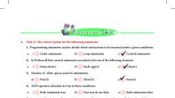
ACTIVITY3: Open the ‘FeeBook’ workbook and use the formulas to calculate the total fee and balance, fee amount of all the students., Format the worksheet as shown here:, •, ,  alculate the total fee under the column, C, head ‘TOTAL’., , , Total=Tution Fee+Bus Fee+Comp, Fee+Fine, •, ,  alculate the balance amount under the, C, column head ‘BALANCE’, Balance=Total ‐ Paid, , Assessment Sheet, A., , Tick () the correct option for the following statements., 1. MS Excel is distributed by this company., , a), , Mitsubishi, , b), , Microsoft, , c), , Apple, , b), , Workbook, , c), , Document, , 2. An Excel file is also called as this., a), , Spreadsheet, , 3. This is not an open source freewere spreadsheet software., a), , Google sheets, , b), , Openoffice‐Calc, , c), , MS Excel, , b), , Column, , c), , Cell, , 4. The basic unit of the spreadsheet., a), , Row, , 5. They are used to perform calculations without typing long and complex formulas., a), , Functions , , b), , Auto Calculators, , c), , Operations, , 6. All the formulas and functions in MS Excel must begin with this sign., a), , @, , b), , #, , c), , =, , c), , colon, , c), , Calculation bar, , 7. In cell reference, this is used to separate the address of two cells., a), , semi colon, , b), , full stop, , 8. The bar that is used to edit or enter the formula or function., a), , Formula bar, , 46 Brainy Gigabyte+ 7, , b), , Function bar

Page 19 :
9. The values in a function on which calculations are performed., a), , Numbers, , b), , Cell values, , c), , Arguments, , 10. The button on the editing group of the home tab used for quick addition of numbers in cells., a), , Auto Add, , b), , AutoSum, , c), , Quick Sum, , c), , AVERAGE, , 11. The function that is used to check a condition., a), , b), , IF, , SUM, , 12. The function that tells you how many entries are there in the specified cells., a), , AVERAGE, , b), , AUTO COUNT, , c), , COUNT, , 13. The formula in C2 is =A2+B2. The change in formula if we copied it in cell C3., a), B., , = A3+B3, , =A?+B?, , c), , = A2+B2, , Give one word answer for the following statements., Help Box, , C., , b), , Plus sign, LibreOffice Calc, Book1, VisiCalc, 16,384, 1,048,576, Tools, , 1. The first computer spreadsheet program., , _____________, , 2. Number of rows in an Excel 2010 sheet., , _____________, , 3. Number of columns in an Excel 2010 sheet., , _____________, , 4. The default name that appears for a new workbook., , _____________, , 5. T,  he option in the Save As dialog box that provides the facility to create the, password to protect a workbook., , _____________, , 6. The shape of the mouse pointer while copying the formula using drag method., , _____________, , 7. Name any open source alternative to MS Excel., , _____________, , Observe the following window and write the output for the formulas/functions given below., 1. =C4*D4, , _____________, , 2. =SUM(E4:E8), , _____________, , 3. =AVERAGE(E4:E8), , _____________, , 4. =MIN(D4:D8), , _____________, , 5. =MAX(E4:E8), , _____________, , 6. =COUNT(A4:A8), , _____________, , 7. =IF(E3>=150,"Out of Budget", "With in Budget"), , _____________, More on MS Excel 47

Page 20 :
D., , E., , F., , Which of the following statements are True or False., 1. In formulas, recalculation is required if we change values in the cells., , _____________, , 2. Cell references in the formulas are not case sensitive., , _____________, , 3. Formula can't be copied to other cells., , _____________, , 4. IF function always returns values either true or false., , _____________, , 5. AutoSum only adds a row of numbers., , _____________, , Write the syntax for following Excel functions., 1. SUM, , Syntax : _____________________________________________________________, , 2. AVERAGE, , Syntax : _____________________________________________________________, , 3. MAX, , Syntax : _____________________________________________________________, , 4. IF, , Syntax : _____________________________________________________________, , Answer the following questions., 1. What is MS Excel? How is it helpful for us?, _______________________________________________________________________________, _______________________________________________________________________________, 2. Why do we need formulas? Write the general rules while typing a formula., _______________________________________________________________________________, _______________________________________________________________________________, 3. Explain different methods of calculating the sum of a range of cells., _______________________________________________________________________________, _______________________________________________________________________________, 4. W,  hat happens if we make the corrections in the data after typing formula? Do we need to type the, formula again or there is some facility in MS Excel to avoid retyping?, _______________________________________________________________________________, _______________________________________________________________________________, 5. What are functions? Explain with an example., _______________________________________________________________________________, _______________________________________________________________________________, 6. What is the difference between protecting a workbook and protecting a worksheet?, _______________________________________________________________________________, _______________________________________________________________________________, 48 Brainy Gigabyte+ 7

Page 21 :
Application Based Questions, 1, ,  ohan is designing a class-wise fee collection, R, report of a school. Study the Excel worksheet as, shown here, carefully and help him to answer the, following questions:, , , a) The formula to find out the total monthly fee of a class., , 2, , Formula, _____________, , Output, _____________, , b) The formula to find out total fee monthly collection of, the class., , _____________, , _____________, , c) The formula to find out the total monthly fee collection, of the school., , _____________, , _____________, , d) The formula to find out the yearly fee collection of the, school., , _____________, , _____________, ,  bserve the following spreadsheet, O, window and help Kanika to write the, correct formulas/functions with their, respective output., , a), , Formula, _____________, , Output, _____________, , b), , _____________, , _____________, , c), , _____________, , _____________, , d), , _____________, , _____________, a, b, c, d, , More on MS Excel 49