Page 1 :
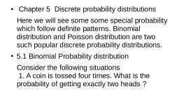
15.7.1, , Theoretical, , probability, , distribution, , in the table, , The probability distribution, as given, of actual observations or by experiments., , above, has, , been, , developed out, distribution or, , However, the probability, considerati0TS On, theoretical, from, purely, of, variables, can, be, interest, developed, many, We, We, distributions., certain assumptions. They are known as theoretical probability, having, shall describe here three such, important theoretical distributions of probability, a wide, range of applications. These are:, 1. Binomial distribution,, , 2. Pois30n, and, 3. Normal distribution., , distribution,

Page 2 :
Cnapier, , Binomial distribution, 15.8, , of the most widely, , e, , This 1, ine, , Out of, , mt (i.c.,, , of1, , experin, , eNale, , male, , o, orr, , a, , cncountered, , process called the, trial) results in only, , a, , female, head, , dead, , tail,, , or, , probability distribution in applicd statistics,, If, , Bernoulli trial., 0ne, , or, , of the, , two, , random process, , a, , mutually, , or, , erclusve outcomes, , then known, alive etc., the trial is, , as, , a, , Bernoulla t r i a l, , Bernoulli, , 1., , of, 2., from, , forms what is, , Sequence of Bernoulli, , the, trials satisfying, , Bernoulli process., erclusive,, in one of two possible, but mutually, Each trial results, other a failure., is termed arbitrarily a success and the, , itions, , c o n d i t, , A, , process, , which, The probability, , of, , following, , called a, , success, , p and that, , of the failure, , q, , (= 1-p), , outcomes, , remain unaltered, , trial to trial., , the outcome of any, implying thereby that, independent,, 3., other trial., not a t e c t e d by the outcome of any, particular trial is, This means to find the, binomial distribution, P(r), for, Expression, in n (n > r), r times exactly, thrice,.,, event, twice,, once,, probability of happening of an, , The trials, , all, , are, , number of trials., , trial is p and the probability, of A is r, Since there are n trials and the happening, 1, is, q., p, happening, of not, this, r times. We may represent, does not happen is 7, times, the number of times it, The probability of happening, , event, , an, , A,, , say in, , one, , =, , -, , -, , pictorially as follows., , (n-r) times, , r times, , A, , indicating the happening, , (15.8.1), , .. AA,, , AAAA.., , AAA..., , and A the failure. Now, the order of arrangement (15.8.1), , above has the probability, p, , PPP, , (7n T ) times, , T times, , But (15.8.1), , is, , just only, , one, , (15.8.2), , qqq*, , order of arranging r, , numbers of A's and, , (n -r), , number, , of A's. There could be many other different arrangements., of, (15.8.1) p"q"-x No. of different arrangements, otA's and (n -r) number of AS., P(r) = "C.p"q", The probability of, , =, , r, , number, , (15.8.3), , = (r +1)th term of (p + q)", distribution., , xpression (15.8.3) is known as the binomial, of happening, IfT, P(0) ""Copq" q" probability, ntri, =, , =, , =, , A 0-times i.e., in all the, , rials, the outcome is a failure., , Ifr, 1, , P(1), , Ifr, **2, P(2), , =, , =, , A 1-time., nCipgn-1 probability of happening, A, "Cop?gn-2 probability of happening 2-times,, =, , =, , and, , so on.

Page 3 :
The above terms are plainly the successive terms in the expansion ot the binomial, , distribution., Bernoulli distribution after Swiss mathcmati, , and hence the name binomial, P+g, T h e distribution is also called the, , cian James Bernoulli who had developed it., , and the cxperiment is repeated, experinent consists of independent trials, s u c c e s s is, number of sets with r, Ntimes, then the frequency ofr success, i.e.,, I t each, , NP(r) = N"Crp'q", , T are given by the, cach, the frequencies of 0, 1,2,3,**,, ot successes, The possible number, Corresponding terms of the expansion of N(p + q)"'., distrabution., the binomial frequency, constitute, with, the, frequencies, expected, along, Hence tor N sets of, , n, , trials, , Fields of, , ypes, , applications, of problems that incude,, , finds applications in many, This binomial distribution, , among ot hers,, , 1. No. of defectives in a sample from production line,, 2. Estimation of reliability of systems., 3. Radar detection, and the, 4. Number of rounds fired from, , following table, , success, , gun, , hitting, , a, , target,, , etc., , Mean of binomial distribution, , 15.8.1, The, , a, , occurs, the, , is rather self-explanatory., , corresponding frequency, , Successes (r), , (f), , It, , gives the, , and the, , number of times, , product, , of, , Frequency (f), , (rf)-value, , npg-1, , Tpg-1, , nan)q-2, 2, , n(n- 1)p?qn-2, , 1, , and, , r, , (r) the, , f., , np, , Efr =npg"-+n(n -1)p°q"-3 +Tn(n-1)(n-2),3-3, 2!, =, , p-1, , np, , nplq + p)", and, , f, , =, , -1)(n-2)3++P, 2!, , 1!, =, , +np-+, , (, , np, , n(, 2!, , p+q= 1), , n - 2 4 +p", , = (g +p)" = 1 (:: p+q= 1), Mean, , of, , binomial distribution, u, , =, , =, , np, , +np"

Page 4 :
Variance and standard deviation of binomial distribution, 1 5 . 8 . 2, , variance and the standard deviation of, derive, to the following table., , To derive the, , Th, , binomial, , distribution,, , we, , take, , recourse, , Successes (r), , (r3f)-value, , Frequency (f), , 0, , 0, , 7pg-l, , 1, , Tnpg-1, , 2, , p-2, , 2(n, , -, , 1)p?q"-2, , n, , p, , '.Total frequency =2f=1, as betore, , rf, , =, , =, , =, , npq, , +2n(n, , np g-1, , ) n - 2 , n - 3 4., , -, , 1)p*g"-24 u3n(n-1)(n-2),3g-3, 2!, , +.+ n^p", , 2n-1), pg-2+.. +np"-1, 1!, , np lg-1, , 1!, , 2 , (T-1)(n2),2n-34++p", , 1, , 2!, , p-2, n-22-1)(7-2,2a-3, 4, +, 2!, , (n -1)p*, , = np|(p+q)*- + (n- 1)p(p + 4)"=, , =, , p+q= 1), np[1 + (n- 1)p] (, (: 1-p= g), , np |np +9, , 2, , (, , Variance, o=, , deviation, a, , Standard, The following, , Worth noting., ., , It is, , a, , characteristics, , r-successes, , The probability of, for S e t s of such trials, the, mean, , in, , independent trials, , distribution, , Standard deviation. is ynp4, distribution, W h e n p = 0.5, the, be the n-value., , n, , theoretical frequency, , of the binomial, , =, , npq, , mpq, , form depends, its general, distribution and, discrete, , 2., , The, , =, , +npq- (np), , binomial distribution, properties of the, , or, , namely p, q and n., , ,, , =np, , is jt, , three, , on, , is given, , are, , parameters,, , and, , by "Crp'q"-, , is N"Cp"q"=r., =, , is symmetrical, , np, its, , ab0ut, , variance, , the, , is npq and, , so, , mean u, whatever, , its, , may

Page 5 :
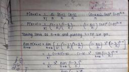
15.9, , Poisson distributioon, , prolbability dlistribution, related, but have a large nunber of independent, , This discrcte, rare, , to, , probabilities of events that, , the, , chances lor, , ocurrence,, , are, , ver, , developed by, , was, , Poisson distribution fro, The best example of, , French mathematician S.D. Poisson., radioactive disintegration., physical science is that of the, The, , of Poisson distribution, , characteristics, , following, , are, , worthy of cOmprehension, becomes, , very very, , 7, binomial distribution, 1. It is the limiting form of the, for cach trial becomes, the constant probability of success, large, i.e., n > o and p,, remains finite., a m a n n e r that np(=m or u), such, in, 0, i.e.,, p>, very small,, is, when, , n, , single parameter, , 2. It cosists of a, , only., , Thc entire, , distribution, , obtained, , very, , once, , the mean jt is known., , probability model in biology, to (i) arrival pattern of, to problems relating, its, applications, from, and medicine, apart, defcctive vehicles in a workshop ctc., (ii) spatial, calls,, telephonic, in, hospitals,, patients, etc., of certain spare parts, distribution of bomb hits, (ii) demand pattern, the Poisson process is described by, used, Poisson distribution has been, , As in binomial distribution,, , Poisson process:, , 1. The, an, , the, , an, , length of the, , interval., , is proportional to the, , Pr), , =, , a, , probability of exactly, already stated,, , Poisson distribution- The, , Expression for, trials in, , second, , same or, , single, , n, , a, , of, , any other interval., of the event must be possible, infinite number of o c c u r r e n c e s, in a given interval, o c c u r r e n c e of the event, of, , in the, , 2. Theoretically, an, in the interval and the probability, , in, , occurrence, , i.e.,, of the event (successes) are independent,, of, on the probability, interval of space and time has no effect, , occurrences, , event in, , Occurrence, , as a, , extensivcly, , binomial distribution, , "Cp'q-, , r!(n -, , is,, , as, , TP(1-P)", , T-successes, , (:p+9=1), , r)!, , n-T, , bn(n-1(n -2)- (n-r+ )1((1-"), replacing np by, , or, , m, , n(n, , -, , p by m/n., , 1)(n, , n n, , n, , 2)...(n r +1) m", -, , -, , r!, , n, , n°, , T, , 1, -T m', , -(1)1-)-1-(1-")"1-), Let, , now n, , oo,, , so, , that, , Pr)= (1 -0)(1, , we, , have, , me-m, , -0)- (1 0)e-m x, -, , Li1, , m, , (1- 0)", =e, , =, , r, , (15.9.1)

Page 6 :
T, , h, , e, , e, , pression (15.9.1) gives, , x, , p, , r, , e, , s, , s, , i, , o, , the Poisson distribution of, , probability of T-success., , that th, the probabilities of 0,1,2,..,T,.. . successes in Poisson distribiition, Note that, , respectively, , by, , given, , P(0)= e"; P(1) = me m; P(2) = me, 2!, , are, , m em, , P3), , =, , m'e, , P(r) =men, , ;, , 3 3!, , etc., , T'he sum of all these probabilities is given by, e, , m, , nem, , me, , n em, , 2!, as, , it should, , be., , have obtained the Poisson distribution, distribution when p -0, n > oo such that np, , It is to be noted also that, , limiting, , =1,, , 3, , case, , of the binomial, , as, , we, , =, , andn p = = m., , 15.9.1, 15.9.1, , Mean and Standard deviation of Poisson distribution, , The mean of the Poisson distribution p is given by, , =pT, , =, , PoT0 +P1T1 +P2T2, , + p3t3 +, m, , 2, , m.0+ mem,1+ * e - , 2 + e .-m.3, 3+., , =, , 3!, , 1, , = me"+ m'e, , m'em +, , 2 70, m2, , e1+m+, me -(e), , =1+m+, , m, , The variance of the Poisson distribution is given by, , =pa- ., NOW,, Now,, , pr = por +pirf +p2rz + P3*3+**, m, , = e 0 + me . 1 +, , 3m, , 2+, , m', , m.32 +..., , 4m3, , me"1+2m+o+ 3, , me, , -m, , 1, , mt m, , 2!, , +, , the, , finite

Page 7 :
m, , =meme+m | 1+ m +, = me, .'a, , =, , m(1, , e, +, , +7me"=1m(1 +m), , pa- 2, , m) m=, -, , S.D =, , Note that in Poisson distribution,, , a, , =, , m, , =, , pr, , Vm, , mean=, , variance, , m., , =, , I n finding the mean and the standard deviation, we could as well take the, , of the binomial distribution, , and make, , that np= m., , oo, p > 0, , n», , Mean,, , Lt(np), , =, , Standard deviation, a, , =, , sults, , 1). We further, , (i.e.,, , note, , m, , =, , Lt (Vnpq) =, , Vm, , Poisson distribution may as well be stated as: 1fr be the number of occurrences, Tundom events in, , of some, , an, , interval, , of time, , or, , space, the, , probability that, , r, , will, , ocCur, , is given by, f(a) =, , eAA, , =, , 0, 1,2,, , (15.9.2), , *,, , number of occurrences, parumeter of the distribution, being the average, of the random event in the given interval., f(r) =1, implying that the distribution, I t can be shown that f(r) 20 and, , where A is the, , (15.9.1), , satisfies the requirements of, , 15.10, We shall, , a, , probability, , distribution., , Normal distribution, consider the most important distribution in statistics, , now, , the, , normas, , distribution- first published by de Moivre. Many other mathematicians, notabl, therefore frequentiy, contributed much to its development. The distribution is, , Gauss,, , referred to, , as, , the Gaussian distribution., , Unlike the previous two, which, , were, , distributions of, , a, , discrete variable, it is, , continuous probability distribution., , be, uwhose variation depends on random c a u s e s will, lts importance lies in that a large, normal distribution., , Any quantity, according to, distributions, , approximate to, , distribute, numoe, , normal distribution., , is, The normal or Gaussian distribution, , defined by, (15.10.1, , -u/2o2, , fr)=y 2To, , arbitrary constants., It is derived as the limiting form of the binomial distribution for large va, , where the, , mean, , and, , thestandard deviationa, , and p, and q are not small., , > 0, , are, , of

Page 8 :
Let, , 18, , v a r i a t e z = (r define aa variate, , define, , u)/a and substitute in (15.10.1) so as to get, , 1, , J:)= 27, h, , (15.10.2)), , is known as the standard form of normal distribution (discussed more in Art., , which, , 10.2 of, , 5 10.1, , this, , Chapter)., , Characteristics (properties) of normal distribution, , 1 5 . 1 0 . 1, , ofthe important characteristic properties of the normal distribution, , Some of t, , Cnie, , curve are, , stated below., , 1. The curve represented by equation (15.10.1) is called the normal probability, , The curve is bell-shaped and symmetrical about its mean ., , As shown in, , curve., , Eo, 15.1, the normal probability curve on either side of 4 is a mirror-image of the, other side., , X, Fig 15.1, , The marimum ordinate is 1/V2To, obtained by puttingr = u, decreasing rapidly, on both-sides of the mean. Its points of inflezion, found by putting d'y/dr2 = 0 and, verifying that these points d'y/dr" # 0, are given by z = pto i.e., equidistant from, the mean on either side., , 2. The mean, the median and the mode, , are, , all, , equal,, , as, , it is, , symmetrical., , The odd order moments about the mean are, , H2n+1, , (-4)T, 2n+1, , V2T J =, , Since the, 0, , 1, V2To, , -/20 dr, , 2n+1e/2 dz,, , where, , z, , =, , (r, , -, , 4)/a, , 0,, , integrand z2n+1e-*/2., , an, , odd function., , normal distribution, all order moments about mean are zero., , Skeuness of the curve B1, , u3/, , = 0., , iane normal distribution is completely determined by the two parameters p and o,, at is,, , se, different normal distribution is specified for each different u and o. Different, s shift the, the graph of the distribution along the r-axis as shown in Fig. 15.2. Different, s ictate, the, t e the different degree of flatness or peakedness of the distribution graph, , g"nd. 15.3)., Math. Phy, , [41)

Page 9 :
2, , Fig 15.2, n, , Fig. 15.2,, , three normal distributions with different means (, ) i l the, i.c., a is shown. Fig. 15.3 shows thee norimal i s t ribat, variability, with different, ions, standard deviations O,O and oa but with, nean 1 . ,, the, same, h e total area, under the curve above the x-axis is one squae, unit. Ifollows, rom the fact, that the normal distribution is a, The, distribution., probability, synmetry, dictates that, me, , drawn, , amount of, , 50% of the, , area, , at the mean., , is to the right and 50% to the left of, , a, , perpendir ular, , 02, , Fig 15.3, , 0.95, , 0.68, , 0.018, , 0.018, , 0.025, , 20, , 10 1, -1o H H+10, , H-20 u, , (a), , (b), , 0.997, , 0.0015, , 30, , 30, H+30, , u-30, (c), Fig 15.4, , 5., , (a) P(4-a, , (b) P(u.- 2o, (c, , Plu-, , <ut a), , < r, <z, , 3d <, , r, , 26, , =, , <u+20), <p+ 3a), , 68%, =, , =, , 95.5%, , 99.7%, , 0.0015, , M+20, , 0.025

Page 10 :
uean th, that, These mean, , if we erect perpendiculars at a distance of a, , i.e., 1 standard, , frotm the mean in both directions, the arca enclosed by the perpendiculars,, yia, and the, the curve will be approximately 68%, of the total arca (Fig. 15.4a). If, T-AXIS and, , distance of 2a, i.c., 2, S.D., on either side of, e aabout 95% of the area will be enclosed (Fig. 15.4b), and extending them a, , boundaries are, neral boun, , extended, , a, , i., the 1of 33a,, 0 , i.c., 3x S.D. will cause approximately 99.7% of the total area being, d, , i, , s, , t, , a, , n, , c, , e, , of, , enclosed (Fig. 15.4c)., Erom, , above,, , it 1s Clear that, , practically all thc, , values of the variable, , r, , lie between, , and 3o with respect to the mcan, in normal distribution. For instance, if the, ts of the Indian adults be normally distributed with mean u 165.28 cm and, heights, e.00 cm, it means that 68% of the adults will have a height bctween 170.28 cm, 160.28 cm and 99.7% will show a height between 180.28 cm to 150.28 cm., =, , 15.10.2, , Standard form of normal distribution, , The characteristic 3 in Art. 15.10.1 implies that the normal distribution is a farnily of, , istributions where one member is distinguished from the other by the values of u and, . The most important member of this family is the standard normal distribution,, also called the unit normal distribution since it has a standard deviation a, mean u, , =, , =, , 1 and, , 0., , The standard normal distribution, as already indicated, can be obtained from, 15.10.1) by substituting a random variable, z, , =, , (r, , -, , u)/o., , The equation for the standard normal distribution i.e., probability density function, Can then be written as, , 1, , f(E) 27, , =e, , -z2/2,, , - O0, , O, , z <, , (15.10.3), , 1, , Fig 15.5, , The, Cgraph, , (or curve) of the standard normal distribution is shown in Fig. 15.5., , The, ne probability of r, , ve, , from, , lying between t1 and t2 is given by the area under the normal, , ri to r2, 1.e.,, , PlrSr ra), , T2e-4)"/20 da:, =, , /2na, , J, , 1 -/2dz, z, , V2T, , =, , (r, , -, , 4)/a, , dz, , =, , dz/a)

Page 11 :
1, , V2T LJo, Pa(z) Pi(2), , =, , where, , Z2, , 2 dz, , Z1, , /2dz\, , Jo, , -, , P() =, , 1, , d, , 2T Jo, , The values of each of the above integrals, are now available in Tables, to the, statisticians. We also give the table, containing different values of z between the, limits, 0 and 3.0, at an interval of 0.05 and the, values of, , corresponding, , The, , function,, , integral, , is known, , =, , V2T Jo, generally denoted, , by f(z),, , Applications, , of normal, applications such as, 1., , Calculation of, , 2., , Computation, , 3. Statistical, , errors, , of, , the, , probability integral, corresponds to Fig. 15.5., as, , distribution- The, , made by chance in all, , probability, , inference, , and, , f{2, , of the hit of, , a, , the, , error, , normal distribution find various, , experimental, , measurements., , shot., , in almost every branch of, , or, , science,, , etc.

Page 12 :
15.4 A, , Example, show, , an even, , that the, , sum, , an, , number than, , of, , an, , biased that when, , so, , odd number., , lf, , throun,, , it is thrown, , twice,, , it is, is tsd, , twice, , on, , throw, , shows an even, , as, , likela, what ic, is the probabilitto, , thrown is odd?, the two numbers, , The biased die, , Solution., , gives, , sir-faced die is, , number, twice, , odd number., Probability of showing an even number, P (even), , 1, , as, , (AMIE, frecmond1., equently as it, , 2, , 2, , 3, 1, Probability of showing an odd number, P, , The, , sum, , (Old), , 7, , 1, , of two numbers is odd if, and the second, , a, , the first is, , (b), , first is odd and the second, , even, , Probability of the, , sum, , P, , odd,, , or, , even., , to be odd is, , P(even) x P (odd) + P (odd)x P (even), , -))-3*i-;, Example 15.5 Calculate the probability of obtaining 4 heads, , in 6, , unbiased coin., Solution., , By, , But, P(r), , the, =, , problem, here,, , p, , =, , $,, , "C,q"=Tp", according, :, , q=, , to, , 6,, , n, , =, , =, , 15x, , (, , r, , =, , 4., , the binomial distribution., , G), , ="Cagp=, , P(4), , 6 and, , 6, , 15, , 64, 64, , tosses, using, , an

Page 13 :
A die is, 15.7 A, ple 15., throuwn 8 times., Ex, Find the probability that 5' will, ezactly, twrce,, tuice, (ii), (ii) at least seven times, 5, show, and (iii) at least once., E x a m p l e, , TH, The, probability of showing 5 in a single trial, hability of not showing a 5 in a, single trial is, , Solution., , is p, , 1/6., , given by, , q=1-p =1-, , 6, , Probability of showing 5 eractly twice in 8, throwsis, P, , =BCap, , L)Probability of showing 5, P, , (ii), , Probability, 8, , times), , is, , of, , =28 (), , at least 7 times, , (), , i.e., 7 times, , Obtain P(X, , 3olution., Solution., , showing, , '5' at least, , once, , P(1) + P(2) + P(3) + ., , 4)., , Since X is, , 8 times is, , -( )+G)-, , 15.8 Let X, =, , or, , =, , +, , (i.e.,, , P(8), , =, , =, , Example, , 68, , P(7)+ P(8) *Cpq+*Cap*g, , =, , given by, , P, , 28x 566, , a, , once,, , 1, , 41, 68, , twice, thrice,, , P(X = 1) = e-", , m, , 1, , =, , follow Poisson distribution such that P(X, , P(X = a) = e-"m",, , =, , /58, -, , 6, , 1), , =, , m, , a = 0,1,2,3,.., , =, , mem, , 1!, , P(X = 2) = e-m, , Now,, , P(X, , = 1), , = P(X = 2) >, , 1, m'em, , e m = 5e-"m, , m = 2, , P(X = 4)e-m m = = z e 22, = =0.090023, 4!, , times,, , P(0), , -, , 1-5Cop°, , Poisson variate with parameter, , 4, , P(X, , =, , 2).

Page 14 :
stributed, , Jldin, , 15.12, , A, , manufacturer produces envelopes whose weight is, normally, with mean =, 1.95 and standard deviation o, 0.05g. The envelopes, lots of 1000. How many envelopes in a lot will be, heavier than 2g? Use the, , Exampl, , =, , followrng fact, , 1, , V2T Jo, Solution., , Given P(0<z< ), Also, given, , u, , 1, , -*/2dx =0.3413, , =, , 2T, , 1.95,, , =, , /2 d =0.3413, , o, , 0.05 and, , =, , x, , =, , 2., , 2-1.95, , =, , 1, , 0.05, , P(z>1), Number of, , envelopes, N, , =, , area of curve right, , =, , =, , 0.5-0.3413, , =, , 0.1587, , heavier than, 1000, , x, , 2g, , 0.1587, , =, , in, , a, , to, , z, , =, , lot of 1000 is, , 158.7, , =, , 159., , 1, , given by