Notes of C2, Economics production and cost..pdf - Study Material
Page 1 :
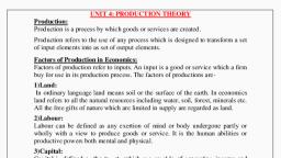
CHAPTER-3, PRODUCTION AND COST, , The production function shows the relationship between input and output. A, production function can be written as:q=f(x1, x2), Where ‘q’ is equal to output ( x1 x2) are the various input/factors, of production., ISOQUANT, An isoquant shows the different combination of two inputs that yield the same, level of output., , The Short Run and The Long Run, In the short run, a firm cannot vary all the input. One factor remain same/fixed in, the short run. The factor that remains fixed is called fixed input. The factor that, the firm can vary is called variable input.
Page 2 :
In the long run, all factors of production can be varied. So in the long run there is, no fixed input., Total Product, Average Product and Marginal Product, Total Product (T.P), The relationship between variable input and output, keeping all other input, constant is refered to as total product of the variable input. It is called total return, or total physical product (TPP)., Average Product (A.P), Average Product is defined as the output per unit of variable input., AP = TP ÷ No of Input, , Marginal Product (M.P), Marginal Product is defined as the change in output per unit of change in the, input., MP = Change in output ÷ Change in input, Or, MP= Δ output ÷ Δ input, Or, MP = TPn-TPn-1, The sum of MP will be the total product., The law of variable proportion or the law of diminishing return, The law of variable proportion or the law of diminishing marginal product states, that when the quantity of one factor is increased keeping the quantity of other, factor fixed, the marginal product of a variable factor increases and after a
Page 3 :
certain stage it starts diminishing. The concept of law of diminishing marginal, product is related to the law of variable proportion., Shapes of TP, MP and AP Curves, The law of variable proportion can be explained with the help of a table and, diagram., Units of labour, , TP, , AP, , MP, , 0, , 0, , 0, , -, , 1, , 20, , 20, , 20, , 2, , 50, , 25, , 30, , 3, , 90, , 30, , 40, , 4, , 120, , 30, , 30, , 5, , 140, , 28, , 20, , 6, , 150, , 25, , 10, , 7, , 150, , 21.4, , 0, , 8, , 140, , 17.4, , -10
Page 4 :
According to the law of variable proportion the marginal product of an output, initially rises and then after a certain stage it starts falling. So marginal product, curve looks like an inverse ‘U’ shaped curve., When we increase the amount of input, the AP also rises. When MP, becomes less than AP, the AP curves also start falling so AP curve is also inverse, ‘U’ shaped., The law of variable proportion has three stages:i), , Stage 1:- Increasing Return/Increase in Returns to a factor, , In this stage, total product increases at an increasing rate. Here, AP and MP increase., ii), , Stage 2:- Diminishing Return/Diminishing returns to a factor, , In this stage, TP increases at a diminishing rate, here AP and MP, FALLS. This stage ends when MP become zero., iii), , Stage 3:- Negative Return
Page 5 :
In this stage, TP declines and MP become negative., The Relation Between AP and MP, i), ii), iii), , When MP>AP, AP rises., When MP=AP, AP will at its maximum., When MP<AP, AP falls., , Relation Between TP and MP, i), ii), iii), iv), , When TP increases at an increasing rate, MP increases., When TP increases at an diminishing rate, MP decreases., When TP reaches the maximum, MP is zero., When TP decreases, MP become negative., , Reasons Behind The Law of Variable Proportion, When we increase the amount of the variable input, the factor proportion, become more and more suitable for the production, so marginal product, increases but after a certain level of employment, the production process become, too crowded with variable input and the factor proportion become less and less, suitable for production, so marginal product starts falling. When more and more, quantity of variable factors are added to the fixed factors, the ratio of proportion, changes, so the law is called the law of variable proportion., Return To Scale [Fixed Proportion:-Long Run Production Function], Return to scale is a long run production function. In the long run all factors of, productions are varied. Returns to scale refers to changes in output when all, inputs are changed in the same proportion., It has three stages:i), , Increasing Returns to Scale [IRS], IRS refers when a proportional increase in all inputs in an increasing, output by more than proportion.
Page 6 :
ii), , iii), , Constant Returns to Scale [CRS], CRS refers when a proportional increase in all inputs results in an, increase in output by same proportion., Decreasing Return to Scale [DRS], , DRS refers when a proportional increase in al inputs results in an, increasing output by less than proportion., These three stages occur due to the operation of economies of scale, and diseconomies of scale., Consider a production function:q=f(x1, x2), When the firm produces ‘q’ amount of output using x 1 amount of factor 1 and, x2 amount of factor 2. Suppose the firm increases both the factor ‘t’, Times, mathematically we can say that production function exhibits constant, returns to scale if we have,, f(tx1, tx2)=tf(x1.x2), Similarly the production function exhibit increasing returns to scale if ,, f(tx1,tx2)>tf(x1.x2), Similarly it exhibit decreasing returns to scale if,, f(tx1,tx2)<tf(x1.x2), Cobb-Douglas Production Function, Consider a production function,, Q=ALα Kβ, OR, , A=Efficiency parameter, L=Labour
Page 7 :
Q= Lα Kβ, , K=Capital, , OR, Q=Xα1Xβ2, Where α and β are constant. The firm produces Q amount of output using, labour (L) and capital (K), this is called Cobb- Douglas Production Function., If we increase both the input ‘t’ times, we get the new output, Q=tα+β.Lα.Kβ, OR, Q=tα+β.xα1.xβ2, When α+β=1, we have constant returns to scale., When α+β>1, we have increasing returns to scale., When α+β<1, we have decreasing returns to scale., COSTS, In order to produce output, the firm needs to employ inputs. A given level of, output can be produced in many ways. A firm will choose that combination of, input which is least expensive. The relationship between output and cost is called, the cost function., Short Run Cost, Total Fixed Cost (TFC), The cost that a firm incurs to employ fixed input is called the total fixed, cost. Whatever may be the level of output, TFC remains the same., Total Variable Cost (TVC)
Page 8 :
The cost that a firm incurs to employ variable input is called the total, variable cost (TVC), Total Cost (TC), The sum of fixed cost and variable cost is called the total cost of a firm., TC=TFC+TVC, When output increases, total variable cost increases so total cost is also, increased. When output is zero, TC=TFC. The relationship between TFC, TC, and, TVC are shown in the following table and diagram., Output, , TFC, , TVC, , TC, , 0, , 100, , 0, , 100, , 1, , 100, , 50, , 150, , 2, , 100, , 70, , 170, , 3, , 100, , 80, , 180, , 4, , 100, , 105, , 205, , 5, , 100, , 135, , 235, , 6, , 100, , 170, , 270
Page 9 :
As output increases TVC and TC increases, TVC and TC have the same shape i.e,, inverse ‘s’ shape. TC starts from the origin of TFC because, when output is 0,, TC=TFC. The TFC curve is parallel to ‘x’ axis because TFC remain the same with the, increase in output., The Short Run Average Cost (SAC), It is the total cost per unit of output., SAC=TC÷Q, SAC*Q=TC, Q= Output Produced, Average Variable Cost (AVC), It is the variable cost per unit of output., AVC=TVC÷Q, AVC*Q=TVC, Average Fixed Cost (AFC), It is the fixed cost per unit of output., AFC=TFC÷Q, AFC*Q=TFC, Short Run Marginal Cost (SMC), It refers to the change in total cost due to change in output., SMC=Change in TC ÷ Change in Q, , i.e, ΔTC÷ΔQ, , OR, SMC= TCn-TCn-1, NB :- The sum of marginal cost gives up total variable cost.
Page 10 :
The following table shows the TFC, TVC, TC, AVC, AFC, MC, ATC., , UNIT OF, OUTPUT, 0, 1, 2, 3, 4, 5, 6, , TFC, , TVC, , TC, , 40, 40, 40, 40, 40, 40, 40, , 0, 60, 80, 90, 110, 150, 200, , 40, 100, 120, 130, 150, 190, 240, , AFC, , AVC, , ATC, , MC, , 40, 20, 13.3, 10, 8, 6.6, , 0, 60, 40, 30, 27.5, 60, 33.3, , 100, 60, 43.3, 37.5, 38, 39.9, , 60, 20, 10, 20, 40, 50, , From the table it is clear that when output increases AFC decreases. As output, move towards to infinity AFC move towards zero. AFC curve is a rectangular, hyperbola i.e, Q*AFC=TFC, , The shape of AVC, SAC, SMC are ‘U’ shaped. When output increases initially AVC, and SMC fall, then it reaches a maximum and start to rise.
Page 11 :
Relationship between MC and AC, When MC<AC, AC falls., When MC=AC, AC will at its minimum., When MC>AC, AC rises., Long Run Cost, In the long run all inputs are variable. So in the long run the total cost and total, variable cost are same. Long Run Average Cost (LRAC) is defined as cost per unit, of output., LRAC= TC÷Q, Shapes of the long run cost curve., The shape of the long run average cost curve is ‘u’ shaped because of the, operation of the return to scale. When increasing return of scale operate, AC falls.
Page 12 :
When constant returns to scale operate AC remain constant. When diminishing, return to scale operate, AC rises. As long as AC is falling, MC must be less than AC., When AC is rising MC must be greater than AC. MC cuts the LRAC at the minimum, point. So long run marginal cost curve is also ‘u’ shaped. This is shown in the, following diagram.
 Learn better on this topic