Page 1 :
F.Y.B.Sc. (CS), SEMESTER - I (CBCS), , DISCRETE MATHEMATICS, SUBJECT CODE : USCS105

Page 3 :
CONTENTS, Unit No., , Title, , Page No., , 1., , Module - I, Recurrence Relations - Functions, , 01, , 2., , Recurrence Relations - Relations, , 06, , 3., , Recurrence Relations -, , 12, , Module - II, 4., , Permutations and Combinations, , 19, , 5., , Counting Principles, , 26, , 6., , Languages, Grammars and Machines, , 32, , Module - III, 7., , Graphs, , 45, , 8., , Trees, , 68, , 

Page 4 :
Syllabus, F.Y.B.Sc. (CS) Discrete Mathematics, Semester I (CBCS), Objectives:, The purpose of the course is to familiarize the prospective learners, with mathematical structures that are fundamentally discrete. This course, introduces sets and functions, forming and solving recurrence relations, and different counting principles. These concepts are useful to study or, describe objects or problems in computer algorithms and programming, languages., Expected Learning Outcomes:, 1) To provide overview of theory of discrete objects, starting with, relations and partially ordered sets., 2) Study about recurrence relations, generating function and operations, on them., 3) Give an understanding of graphs and trees, which are widely used in, software., 4) Provide basic knowledge about models of automata theory and the, corresponding formal languages., Unit I :, Recurrence Relations, (a) Functions: Definition of function. Domain, co domain and the range of, a function. Direct and inverse images. Injective, surjective and bijective, functions. Composite and inverse functions., (b) Relations: Definition and examples. Properties of relations , Partial, Ordering sets, Linear Ordering Hasse Daigrams, Maximum and Minimum, elements, Lattices, (c) Recurrence Relations: Definition of recurrence relations, Formulating, recurrence relations, solving recurrence relations- Back tracking method,, Linear homogeneous recurrence relations with constant coefficients., Solving linear homogeneous recurrence relations with constant, coefficients of degree two when characteristic equation has distinct roots, and only one root, Particular solutions of non linear homogeneous, recurrence relation, Solution of recurrence relation by the method of, generation functions, Applications- Formulate and solve recurrence, relation for Fibonacci numbers, Tower of Hanoi, Intersection of lines in a, plane, Sorting Algorithms., Unit II, Counting Principles, Languages and Finite State Machine, (a) Permutations and Combinations: Partition and Distribution of objects,, Permutation with distinct and indistinct objects, Binomial numbers,, Combination with identities : Pascal Identity, Vandermonde’s Identity,, Pascal triangle, Binomial theorem, Combination with indistinct objects., (b) Counting Principles: Sum and Product Rules, Two-way counting, Tree, diagram for solving counting problems, Pigeonhole Principle (without, I

Page 5 :
proof); Simple examples, Inclusion Exclusion Principle (Sieve formula), (Without proof)., (c) Languages, Grammars and Machines: Languages, regular Expression, and Regular languages, Finite state Automata, grammars, Finite state, machines, Gödel numbers, Turing machines., Unit III, Graphs and Trees, (a) Graphs : Definition and elementary results, Adjacency matrix, path, matrix, Representing relations using diagraphs, Warshall’s algorithm shortest path, Linked representation of a graph, Operations on graph with, algorithms - searching in a graph; Insertion in a graph, Deleting from a, graph, Traversing a graph- Breadth-First search and Depth-First search., (b) Trees: Definition and elementary results. Ordered rooted tree, Binary, trees, Complete and extended binary trees, representing binary trees in, memory, traversing binary trees, binary search tree, Algorithms for, searching and inserting in binary search trees, Algorithms for deleting in a, binary search tree, Text books:, 1. Discrete Mathematics and Its Applications, Seventh Edition by, Kenneth H. Rosen, McGraw Hill Education (India) Private Limited., (2011), 2. Norman L. Biggs, Discrete Mathematics, Revised Edition, Clarendon, Press, Oxford 1989., 3. Data Structure Seymor Lipschutz, Schaum’s out lines, McGraw-Hill, Inc., Additional References:, 1. Elements of Discrete Mathematics: C.L. Liu , Tata McGraw- Hill, Edition ., 2. Concrete Mathematics (Foundation for Computer Science): Graham,, Knuth, Patashnik Second Edition, Pearson Education., 3. Discrete Mathematics : Semyour Lipschutz, Marc Lipson, Schaum’s, out lines, McGraw - Hill Inc., 4. Foundations in Discrete Mathematics: K.D. Joshi, New Age, Publication, New Delhi., , , , II

Page 6 :
Module I, Recurrence Relations, , 1, FUNCTIONS, Unit Structure:, 1.1.1 Introduction., 1.1.2 Functions., 1.1.3 Domain, Co-domain and the range of a function., 1.1.4 Injective, surjective and bijective functions., 1.1.5 Composite and inverse functions, 1.1.5 Summary, 1.1.6 Exercise, 1.1.7 Reference., , 1.1.1 INTRODUCTION, In many instances we assign to each element of a set a particular, element of a second set (which may be the same as the first). For example,, suppose that each student in a discrete mathematics class is assigned a, letter grade from the set {A, B, C, D, F}. And suppose that the grades are, A for Adams, C for Chou, B for Good friend, A for Rodriguez, and F for, Stevens., , 1.1.2 FUNCTIONS, Let A and B be nonempty sets. A function f from A to B is an assignment, of exactly one element of B to each element of A. We write f (a) = b if b is, the unique element of B assigned by the function f to the element a of A., If f is a function from A to B, we write f : A → B. Functions are, sometimes also called mappings or transformations., e.g. f(x) = x2 shows us that function "f" takes "x" and squares it. Here f, stands for function; x stands for input; x2 stands for output., f(x) = x2, , 1

Page 7 :
Function, Input, 0, 1, 2, 3, 4, 5, …, , Input, Relationship, x2, x2, x2, x2, x2, x2, x2, , Output, Output, 0, 1, 4, 9, 16, 25, …, , Functions are specified in many different ways. Sometimes we, explicitly state the assignments, as in Figure 1. Often we give a formula,, such as f (x) = x + 1, to define a function. Other times we use a computer, program to specify a function., If f is a function from A to B, we say that A is the domain of f and, B is the codomain of f. If f (a) = b, we say that b is the image of a and a is, a preimage of b. The range, or image, of f is the set of all images of, elements of A. Also, if f is a function from A to B, we say that f maps A, to B., , 1.1.3 DOMAIN, CO-DOMAIN AND THE RANGE OF A, FUNCTION, Let G be the function that assigns a grade to a student in our, discrete mathematics class. Note that G(Adams) = A, for instance. The, domain of G is the set {Adams, Chou, Goodfriend, Rodriguez, Stevens},, and the codomain is the set {A, B, C, D, F}. The range of G is the set {A,, B, C, F}, because each grade except D is assigned to some student., Generally function is called as domain. The Possible outcome is, called as co-domain. The actual outcome is called as range of a function., Consider a function f(x) = 2x + 1, , 1, , 1, 2, 3, 4, 5, 6, B, 7, 8, 9, , 2, 3, 4, , A, , 2

Page 8 :
In above example A = {1, 2, 3, 4 } is domain , B = {1,2,3,4,5,6,7,8,9} is a, co-domain and Range = {3, 5, 7, 9}, Range is calculated in following manner:, f(x) = 2x + 1 …. For x =1 …… f(1) = 2 (1) + 1= 2 + 1 = 3, f(x) = 2x + 1 …. For x =2 …… f(1) = 2 (2) + 1= 4 + 1 = 5, f(x) = 2x + 1 …. For x =3 …… f(1) = 2 (3) + 1= 6 + 1 = 7, f(x) = 2x + 1 …. For x =4 …… f(1) = 2 (4) + 1= 8 + 1 = 9, , 1.1.4 INJECTIVE,, FUNCTIONS, , SURJECTIVE, , AND, , BIJECTIVE, , Injective, A function f is injective if and only if whenever f(x) = f(y), x = y., Example: f(x) = x+5 from the set of real numbers real numbers to real, numbers is an injective function., Is it true that whenever f(x) = f(y), x = y ?, Imagine x=3, then:, f(x) = 8, Now I say that f(y) = 8, what is the value of y? It can only be 3, so x=y, Surjective, A function f (from set A to B) is surjective if and only if for every, y in B, there is at least one x in A such that f(x) = y, in other words f is, surjective if and only if f(A) = B., In simple terms: every B has some A., Example: The function f(x) = 2x from the set of natural numbers natural, numbers to the set of non-negative even numbers is a surjective function., BUT f(x) = 2x from the set of natural numbers natural numbers to natural, numbers is not surjective, because, for example, no member in natural, numbers can be mapped to 3 by this function., Bijective, A function f (from set A to B) is bijective if, for every y in B, there is, exactly one x in A such that f(x) = y, Alternatively, f is bijective if it is a one-to-one correspondence between, those sets, in other words both injective and surjective., Example: The function f(x) = x2 from the set of positive real numbers to, positive real numbers is both injective and surjective. Thus it is also, bijective., But the same function from the set of all real numbers real, numbers is not bijective because we could have, for example, both, f(2)=4 and, f(-2)=4, 3

Page 9 :
1.1.5 COMPOSITE AND INVERSE FUNCTIONS, The process of combining functions so that the output of one, function becomes the input of another is known as a composition of, functions. The resulting function is known as a composite function. We, represent this combination by the following notation:, (f∘ g)(x) =f(g(x)), We read the left-hand side as “ f“ composed with g at x , and, the right-hand side as “ f of g of x .” The two sides of the equation have, the same mathematical meaning and are equal. The open circle symbol, ∘, , is called the composition operator. Composition is a binary operation that, takes two functions and forms a new function, much as addition or, multiplication takes two numbers and gives a new number., If f(x)=−2xf(x)=−2x and g(x)=x2−1g(x)=x2−1,, evaluate f(g(3))f(g(3)) and g(f(3))g(f(3))., To evaluate f(g(3))f(g(3)), first substitute, or input the value, of 33 into g(x)g(x) and find the output. Then substitute that value into, the f(x)f(x) function, and simplify:, g(3)=(3)2−1=9−1=8g(3)=(3)2−1=9−1=8, f(8)=−2(8)=−16f(8)=−2(8)=−16, Therefore, f(g(3))=−16f(g(3))=−16, To evaluate g(f(3))g(f(3)), find f(3)f(3) and then use that output value as, the input value into the g(x)g(x) function:, f(3)=−2(3)=−6f(3)=−2(3)=−6, g(−6)=(−6)2−1=36−1=35g(−6)=(−6)2−1=36−1=35, Therefore, g(f(3))=35g(f(3))=35, An inverse function, which is notated f−1(x)f−1(x), is defined as the, inverse function of f(x)f(x) if it consistently reverses the f(x)f(x) process., That is, if f(x)f(x) turns aa into bb, then f−1(x)f−1(x) must turn bb into aa., More concisely and formally, f−1(x)f−1(x) is the inverse function, of f(x)f(x) if:, f(f−1(x))=xf(f−1(x))=x, Below is a mapping of function f(x)f(x) and its inverse, function, f−1(x)f−1(x). Notice that the ordered pairs are reversed from the, original function to its inverse. Because f(x)f(x) maps aa to 33, the, inverse f−1(x)f−1(x) maps 33 back to aa., 4

Page 10 :
1.2.5 SUMMARY, This chapter gives introductory review on functions and their, examples. It will create base for advanced level., , 1.2.6 EXERCISE, 1. Specify a codomain for each. Under what conditions is each of these, functions withthe codomain you specified onto?, 2. Specify a codomain for each. Under what conditions is each of the, functions with the codomain you specified onto?, 3. Give an example of a function from N to N that is, a) one-to-one but not onto., b) onto but not one-to-one., c) both onto and one-to-one (but different from the identity function)., d) neither one-to-one nor onto., 4. Give an explicit formula for a function from the set ofintegers to the set, of positive integers that is, a) one-to-one, but not onto., b) onto, but not one-to-one., c) one-to-one and onto., d) neither one-to-one nor onto, , 1.2.7 REFERENCES:1. Discrete Mathematics and Its Applications, Seventh Edition by Kenneth, H. Rosen, McGraw Hill Education (India) Private Limited. (2011), 2. Norman L. Biggs, Discrete Mathematics, Revised Edition, Clarendon, Press, Oxford 1989., 3. Data Structures Seymour Lipschutz, Schaum’s out lines, McGraw- Hill, Inc., 4. Elements of Discrete Mathematics: C.L. Liu , Tata McGraw- Hill, Edition ., 5. Concrete Mathematics (Foundation for Computer Science): Graham,, Knuth, Patashnik Second Edition, Pearson Education., 6., , Discrete Mathematics: Semyour Lipschutz, Marc Lipson, Schaum’s, out lines, McGraw- Hill Inc., , 7. Foundations in Discrete Mathematics: K.D. Joshi, New Age, Publication, New Delhi., , , , 5

Page 11 :
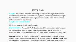
2, RELATIONS, Unit Structure: 1.2.1 Introduction., 1.2.2 Partial Ordering Set., 1.2.3 Hasse Diagram., 1.2.4 Maximum and Minimum Element, 1.2.5 Summary, 1.2.6 Exercise, 1.2.7 Reference., , 1.2.1 INTRODUCTION, A relation between two sets is a collection of ordered pairs, containing one object from each set. If the object x is from the first set and, the object y is from the second set, then the objects are said to be related if, the ordered pair (x,y) is in the relation. A function is a type of relation., , 1.2.2 PARTIAL ORDERING SET, DEFINITION 1 A relation R on a set S is called a partial ordering or, partial order if it is reflexive, antisymmetric, and transitive. A set S, together with a partial ordering R is called a partially ordered set, or poset,, and is denoted by (S, R). Members of S are called elements of the poset., EXAMPLE 1 Show that the “greater than or equal” relation (≥) is a, partial ordering on the set of integers. Solution: Because a ≥ a for every, integer a, ≥ is reflexive. If a ≥ b and b ≥ a, then a = b. Hence, ≥ is, antisymmetric. Finally, ≥ is transitive because a ≥ b and b ≥ c imply that a, ≥ c. It follows that ≥ is a partial ordering on the set of integers and (Z, ≥) is, a poset, EXAMPLE 2 Show that the inclusion relation ⊆ is a partial ordering on, the power set of a set S. Solution: Because A ⊆ A whenever A is a subset, of S, ⊆ is reflexive. It is antisymmetric because A ⊆ B and B ⊆ A imply, that A = B. Finally, ⊆ is transitive, because A ⊆ B and B ⊆ C imply that, A ⊆ C. Hence, ⊆ is a partial ordering on P (S), and (P (S), ⊆) is a poset., DEFINITION 2 The elements a and b of a poset (S, ) are called, comparable if either a b or b a. When a and b are elements of S such that, neither a b nor b a, a and b are called incomparable. EXAMPLE 5 In the, 6

Page 12 :
poset (Z+, |), are the integers 3 and 9 comparable? Are 5 and 7, comparable? Solution: The integers 3 and 9 are comparable, because 3 | 9., The integers 5 and 7 are incomparable, because 5 | 7 and 7 | 5. ▲ The, adjective “partial” is used to describe partial orderings because pairs of, elements may be incomparable. When every two elements in the set are, comparable, the relation is called a total ordering, , 1.2.3 HASSE DIAGRAMS, Many edges in the directed graph for a finite poset do not have to, be shown because they must be present. For instance, consider the directed, graph for the partial ordering {(a, b) | a ≤ b} on the set {1, 2, 3, 4}, shown, in Figure 2(a). Because this relation is a partial ordering, it is reflexive,, and its directed graph has loops at all vertices. Consequently, we do not, have to show these loops because they must be present; in Figure 2(b), loops are not shown. Because a partial ordering is transitive, we do not, have to show those edges that must be present because of transitivity. For, example, in Figure 2(c) the edges (1, 3), (1, 4), and (2, 4) are not shown, because they must be present. If we assume that all edges are pointed, “upward” (as they are drawn in the figure), we do not have to show the, directions of the edges; Figure 2(c) does not show directions. In general,, we can represent a finite poset (S, ) using this procedure: Start with the, directed graph for this relation. Because a partial ordering is reflexive, a, loop (a, a) is present at every vertex a. Remove these loops. Next, remove, all edges that must be in the partial ordering because of the presence of, other edges and transitivity. That is, remove all edges (x, y) for which, there is an element z ∈ S such that x ≺ z and z ≺ x. Finally, arrange each, edge so that its initial vertex is below its terminal vertex (as it is drawn on, paper). Remove all the arrows on the directed edges, because all edges, point “upward” toward their terminal vertex. These steps are well defined,, and only a finite number of steps need to be carried out for a finite poset., When all the steps have been taken, the resulting diagram contains, sufficient information to find the partial ordering, as we will explain later., The resulting diagram is called theHasse diagram of(S, ), named after the, twentieth-century German mathematician Helmut Hasse who made, extensive use of them. Let (S, ) be a poset. We say that an element y ∈ S, covers an element x ∈ S if x ≺ y and there is no element z ∈ S such that x, ≺ z ≺ y. The set of pairs (x, y) such that y covers x is called the covering, relation of (S, ). From the description of the Hasse diagram of a poset, we, see that the edges in the Hasse diagram of (S, ) are upwardly pointing, edges corresponding to the pairs in the covering relation of (S, )., Furthermore, we can recover a poset from its covering relation, because it, is the reflexive transitive closure of its covering relation. (Exercise 31 asks, for a proof of this fact.) This tells us that we can construct a partial, ordering from its Hasse diagram., , 7

Page 13 :
EXAMPLE 12 Draw the Hasse diagram representing the partial ordering, {(a, b)|a divides b} on, {1, 2, 3, 4, 6, 8, 12}., Solution: Begin with the digraph for this partial order, as shown in Figure, 3(a). Remove all loops, as shown in Figure 3(b). Then delete all the edges, implied by the transitive property. These are (1, 4), (1, 6), (1, 8), (1, 12),, (2, 8), (2, 12), and (3, 12). Arrange all edges to point upward, and delete, all arrows to obtain the Hasse diagram. The resulting Hasse diagram is, shown in Figure 3(c)., , 1.2.4 MAXIMUM AND MINIMUM ELEMENTS, Elements of posets that have certain extremal properties are, important for many applications. An element of a poset is called maximal, if it is not less than any element of the poset. That is, a is maximal in the, poset (S, ) if there is no b ∈ S such that a ≺ b. Similarly, an element of a, poset is called minimal if it is not greater than any element of the poset., That is, a is minimal if there is no element b ∈ S such that b ≺ a. Maximal, , 8

Page 14 :
and minimal elements are easy to spot using a Hasse diagram. They are, the “top” and “bottom” elements in the diagram., EXAMPLE 1 : Which elements of the poset ({2, 4, 5, 10, 12, 20, 25}, |), are maximal, and which are minimal? Solution: The Hasse diagram in, Figure 5 for this poset shows that the maximal elements are 12, 20, and, 25, and the minimal elements are 2 and 5. As this example shows, a poset, can have more than one maximal element and more than one minimal, element. Sometimes there is an element in a poset that is greater than, every other element. Such an element is called the greatest element. That, is, a is the greatest element of the poset (S, ≺), Lattices, A partially ordered set in which every pair of elements has both a, least upper bound and a greatest lower bound is called a lattice. Lattices, have many special properties. Furthermore, lattices are used in many, different applications such as models of information flow and play an, important role in Boolean algebra., EXAMPLE 2 Determine whether the posets represented by each of the, Hasse diagrams in Figure 8 are lattices. Solution: The posets represented, by the Hasse diagrams in (a) and (c) are both lattices because in each poset, every pair of elements has both a least upper bound and a greatest lower, bound, as the reader should verify. On the other hand, the poset with the, Hasse diagram shown in (b) is not a lattice, because the elements b and c, have no least upper bound. To see this, note that each of the elements d, e,, and f is an upper bound, but none of these three elements precedes the, other two with respect to the ordering of this poset., , 1.2.5 SUMMARY, Relationships among elements of more than two sets often arise., For instance, there is a relationship involving the name of a student, the, student’s major, and the student’s grade point average., , 9

Page 15 :
Si, milarly, there is a relationship involving the airline, flight number, starting, point, destination, departure time, and arrival time of a flight. An example, of such a relationship in mathematics involves three integers, where the, first integer is larger than the second integer, which is larger than the third., Another example is the betweenness relationship involving points on a, line, such that three points are related when the second point is between, the first and the third., , 1.2.6 EXERCISE, 1. List the ordered pairs in the relation R fromA = {0, 1, 2, 3, 4} to B = {0,, 1, 2, 3}, where (a, b) ∈ Rif and only if, a) a = b., b) a + b = 4., c) a>b., d) a | b., e) gcd(a, b) = 1., f ) lcm(a, b) = 2., 2. a) List all the ordered pairs in the relationR = {(a, b) | a divides b} on, the set {1, 2, 3, 4, 5, 6}., b) Display this relation graphically., c) Display this relation in tabular form., 3. For each of these relations on the set {1, 2, 3, 4}, decidewhether it is, reflexive, whether it is symmetric, whetherit is antisymmetric, and, whether it is transitive., a) {(2, 2), (2, 3), (2, 4), (3, 2), (3, 3), (3, 4)}, b) {(1, 1), (1, 2), (2, 1), (2, 2), (3, 3), (4, 4)}, c) {(2, 4), (4, 2)}, d) {(1, 2), (2, 3), (3, 4)}, e) {(1, 1), (2, 2), (3, 3),(4, 4)}, f ) {(1, 3), (1, 4), (2, 3), (2, 4), (3, 1), (3, 4)}, 4. Determine whether the relation R on the set of all peopleis reflexive,, symmetric, antisymmetric, and/or transitive, where (a, b) ∈ R if and only, if, a) a is taller than b., b) a and b were born on the same day., c) a has the same first name as b., d) a and b have a common grandparent., , 10

Page 16 :
5. Determine whether the relation R on the set of all Webpages is, reflexive, symmetric, antisymmetric, and/or transitive, where (a, b) ∈ R if, and only if, a) everyone who has visited Web page a has also visitedWeb page b., b) there are no common links found on both Webpage a and Web page b., c) there is at least one common link on Web page a andWeb page b, , 1.2.7 REFERENCES:1. Discrete Mathematics and Its Applications, Seventh Edition by Kenneth, H. Rosen, McGraw Hill Education(India) Private Limited. (2011), 2. Norman L. Biggs, Discrete Mathematics, Revised Edition, Clarendon, Press, Oxford 1989., 3. Data Structures Seymour Lipschutz, Schaum’s out lines, McGraw- Hill, Inc., 4. Elements of Discrete Mathematics: C.L. Liu , Tata McGraw- Hill, Edition ., 5. Concrete Mathematics (Foundation for Computer Science): Graham,, Knuth, Patashnik Second Edition,Pearson Education., 6. Discrete Mathematics: Semyour Lipschutz, Marc Lipson, Schaum’s out, lines, McGraw- Hill Inc., 7. Foundations in Discrete Mathematics: K.D. Joshi, New Age, Publication, New Delhi., , , , 11

Page 17 :
3, RECURRENCE RELATION, Unit Structure: 3.3.1 Introduction., 3.3.2 Recurrence Relation., 3.3.3 Linear homogeneous recurrence relations with constant, coefficients., 3.3.4 Solving Linear Recurrence Relations., 3.3.5 Linear No homogeneous Recurrence Relations with Constant, Coefficients., 3.3.6 Summary, 3.3.7 Exercise, 1.3.8 References, , 3.3.1INTRODUCTION, This chapter is focusing on Recurrence relations and example, , 3.3.2 RECURRENCE RELATION, A recurrence relation is an equation that recursively defines a, sequence where the next term is a function of the previous terms, (Expressing Fnas some combination of Fi with i<n)., Example − Fibonacci series − Fn=Fn−1+Fn−2, Tower of Hanoi − Fn=2Fn−1+1, Linear Recurrence Relations, A linear recurrence equation of degree k or order k is a recurrence, equation which is in the format xn=A1xn−1+A2xn−1+A3xn−1+…Akxn−k(An, is a constant and Ak≠0) on a sequence of numbers as a first-degree, polynomial., These are some examples of linear recurrence equations, , 12

Page 18 :
Three cases may occur while finding the roots −, Case 1 − If this equation factors as (x−x1)(x−x1)=0 and it produces two, distinct real roots x1 and x2, then Fn=axn1+bxn2 is the solution. [Here, a, and b are constants], Case 2 − If this equation factors as (x−x1)2=0 and it produces single real, root x1, then Fn=axn1+bnxn1 is the solution., Case 3 − If the equation produces two distinct complex roots, x1 and x2 in, polar form x1=r∠θ and x2=r∠(−θ), then Fn=rn(acos(nθ)+bsin(nθ)) is the, solution., Problem 1, Solve the recurrence relation Fn=5Fn−1−6Fn−2 where F0=1 and F1=4, Solution, The characteristic equation of the recurrence relation is −, x2−5x+6=0,, So, (x−3)(x−2)=0, Hence, the roots are −, x1=3 and x2=2, The roots are real and distinct. So, this is in the form of case 1, Hence, the solution is −, Fn=axn1+bxn2, Here, Fn=a3n+b2n (As x1=3 and x2=2), Therefore,, 1=F0=a30+b20=a+b, 4=F1=a31+b21=3a+2b, Solving these two equations, we get a=2 and b=−1, Hence, the final solution is −, Fn=2.3n+(−1).2n=2.3n−2n, A recurrence relation is an equation that recursively defines a, sequence, i.e., each term of the sequence is defined as a function of the, preceding terms. A recursive formula must be accompanied by initial, conditions (information about the beginning of the sequence).The first, method is called backtracking, and consists of taking a linear recurrence, defining an, and replace the terms an−1, an−2, . . . with the relation that, defines an, but where n is replaced by n − 1, n − 2, etc. This is best, illustrated on an example., Example 61. Consider the linear recurrence, an = an−1 + 3, a1 = 2., Then an−1 = an−2 + 3 an−2 = an−3 + 3 an−3 = an−4 + 3 and so on and so forth., 13

Page 19 :
Therefore an = an−1 + 3 = (an−2 + 3) + 3 = an−2 + 2 · 3 = (an−3 + 3) + 6 = an−3, + 3 · 3 = . . . = a1 + 3(n − 1)., The last equality follows because a generic term is of the form an−i+ 3i,, therefore when n − i = 1, i = n − 1. By plugging the initial condition, we, conclude an = 2 + 3(n − 1)., Once the solution has been found, you may wonder how to check whether, this is the right answer. One way to do it is by proving it by induction!, , 3.3.3, LINEAR, HOMOGENEOUS, RECURRENCE, RELATIONS WITH CONSTANT COEFFICIENTS, A linear homogeneous relation of degree d is of the form, an = c1an-1+c2an-2+…..+cdan-d, Example 63. The Fibonacci sequence fn= fn−1 + fn−2 is a homogeneous, relation. Let us compute its characteristic equation:, xn − xn−1 − xn−2 = 0 ⇐⇒ xn−2, (x2 − x − 1) = 0, therefore x2 − x − 1 = 0 is the characteristic equation., Let us focus on quadratic characteristic equations, that is of the formx2 −, c1x − c2 = 0which corresponds to linear recurrences of the form, an = c1an−1 + c2an−2., Suppose that x2 − c1x − c2 = 0 has two distinct real roots s1, s2, then, s21 − c1s1 − c2 = 0, s22 − c1s2 − c2 = 0., Thereforesn1 − c1sn−11 − c2sn−2 = 0, sn2 − c1sn−12 − c2sn−2 = 0, and we have that if s is a solution of x2 −c1x−c2 = 0 then snis a solution, ofan = c1an−1+c2an−2. This tells us that solutions of an are composed of, sn1, sn2., Note the term ”composed” is used, because if a sequence a0nbalso, satisfies therecurrence of an, then an + a’nsatisfies the recurrence of an as, well, as doesmultiples of an, , 3.3.4 SOLVING LINEAR RECURRENCE RELATIONS:A linear homogeneous recurrence relation of degree k with, constant coefficients is a recurrence relation of the form an = c1an−1 + c2an−2, +···+ ckan−k,where c1, c2,...,ck are real numbers, and ck ≠ 0, The recurrence relation in the definition is linear because the righthand side is a sum of previous terms of the sequence each multiplied by a, function of n. The recurrence relation is homogeneous because no terms, occur that are not multiples of the aj s. The coefficients of the terms of the, sequence are all constants, rather than functions that depend on n. The, 14

Page 20 :
degree is k because an is expressed in terms of the previous k terms of the, sequence., A consequence of the second principle of mathematical induction, is that a sequence satisfying the recurrence relation in the definition is, uniquely determined by this recurrence relation and the k initial conditions, a0 = C0, a1 = C1,...,ak−1 = Ck−1.EXAMPLE 1 The recurrence relation Pn =, (1.11)Pn−1 is a linear homogeneous recurrence relation of degree one. The, recurrence relation fn = fn−1 + fn−2 is a linear homogeneous recurrence, relation of degree two. The recurrence relation an = an−5 is a linear, homogeneous recurrence relation of degree five., Example 2 presents some examples of recurrence relations that are not, linear homogeneous recurrence relations with constant coefficients, , 3.3.5 LINEAR NONHOMOGENEOUS RECURRENCE, RELATIONS WITH CONSTANT COEFFICIENTS, We have seen how to solve linear homogeneous recurrence relations with, constant coefficients. Is there a relatively simple technique for solving a, linear, but not homogeneous, recurrence relation with constant, coefficients, such as an = 3an−1 + 2n? We will see that the answer is yes for, certain families of such recurrence relations. The recurrence relation an =, 3an−1 + 2n is an example of a linear nonhomogeneous recurrence relation, with constant coefficients, that is, a recurrence relation of the form an =, c1an−1 + c2an−2 +···+ ckan−k + F (n),, where c1, c2,...,ck are real numbers and F (n) is a function not identically, zero depending only on n. The recurrence relation an = c1an−1 + c2an−2 +···+, ckan−k is called the associated homogeneous recurrence relation. It plays an, important role in the solution of the nonhomogeneous recurrence relation., Merge Sort The merge sort algorithm (introduced in Section 5.4) splits a, list to be sorted with n items, where n is even, into two lists with n/2, elements each, and uses fewer than n comparisons to merge the two sorted, lists of n/2 items each into one sorted list. Consequently, the number of, comparisons used by the merge sort to sort a list of n elements is less than, M(n), where the function M(n) satisfies the divide-and-conquer recurrence, relation M(n) = 2M(n/2) + n., Tower of Honoi, The Tower of Hanoi A popular puzzle of the late nineteenth, century invented by the French mathematician Édouard Lucas, called the, Tower of Hanoi, consists of three pegs mounted on a board together with, disks of different sizes. Initially these disks are placed on the first peg in, order of size, with the largest on the bottom (as shown in Figure 2). The, rules of the puzzle allow disks to be moved one at a time from one peg to, another as long as a disk is never placed on top of a smaller disk. The goal, of the puzzle is to have all the disks on the second peg in order of size,, 15

Page 21 :
with the largest on the bottom. Let Hn denote the number of moves needed, to solve the Tower of Hanoi problem with n disks. Set up a recurrence, relation for the sequence {Hn}. Solution: Begin with n disks on peg 1. We, can transfer the top n − 1 disks, following the rules of the puzzle, to peg 3, using Hn−1 moves (see Figure 3 for an illustration of the pegs and disks at, this point). We keep the largest disk fixed during these moves. Then, we, use one move to transfer the largest disk to the second peg. We can, transfer the n − 1 disks on peg 3 to peg 2 using Hn−1 additional moves,, placing them on top of the largest disk, which always stays fixed on the, bottom of peg 2. Moreover, it is easy to see that the puzzle cannot be, solved using fewer steps. This shows that Hn= 2Hn−1 + 1. The initial, condition is H1 = 1, because one disk can be transferred from peg 1 to peg, 2, according to the rules of the puzzle, in one move, , We can use an iterative approach to solve this recurrence relation. Note, that Hn = 2Hn−1 + 1 = 2(2Hn−2 + 1) + 1 = 22Hn−2 + 2 + 1 = 22(2Hn−3 + 1) +, 2 + 1 = 23Hn−3 + 22 + 2 + 1 . . . = 2n−1H1 + 2n−2 + 2n−3 +···+ 2 + 1 =, 2n−1 + 2n−2 +···+ 2 + 1 = 2n − 1. We have used the recurrence relation, repeatedly to express Hn in terms of previous terms of the sequence. In the, next to last equality, the initial condition H1 = 1 has been used. The last, equality is based on the formula for the sum of the terms of a geometric, series, which can be found in Theorem 1 in Section 2.4. The iterative, approach has produced the solution to the recurrence relation Hn = 2Hn−1, + 1 with the initial condition H1 = 1. This formula can be proved using, mathematical induction. This is left for the reader as Exercise 1. A myth, created to accompany the puzzle tells of a tower in Hanoi where monks, 16

Page 22 :
are transferring 64 gold disks from one peg to another, according to the, rules of the puzzle. The myth says that the world will end when they finish, the puzzle. How long after the monks started will the world end if the, monks take one second to move a disk? From the explicit formula, the, monks require 264 − 1 = 18,446,744,073,709,551,615 moves to transfer, the disks. Making one move per second, it will take them more than 500, billion years to complete the transfer, so the world should survive a while, longer than it already has, , 3.3.6 SUMMARY, This chapter gives introductory view about recurrence relation and, also explains and demonstrates some basic examples., , 3.3.7 EXERCISE, 1. Use mathematical induction to verify the formula derivedin Example 2, for the number of moves required to complete the Tower of Hanoi, puzzle., 2. a) Find a recurrence relation for the number of permutations of a set, with n elements., b) Use this recurrence relation to find the number of permutations of a set, with n elements using iteration., 3. A vending machine dispensing books of stamps acceptsonly one-dollar, coins, $1 bills, and $5 bills., a) Find a recurrence relation for the number of waysto deposit n dollars in, the vending machine, wherethe order in which the coins and bills are, depositedmatters., b) What are the initial conditions?, c) How many ways are there to deposit $10 for a bookof stamps?, 4. A country uses as currency coins with values of 1 peso,2 pesos, 5 pesos,, and 10 pesos and bills with values of5 pesos, 10 pesos, 20 pesos, 50, pesos, and 100 pesos. Finda recurrence relation for the number of, ways to pay a billof n pesos if the order in which the coins and bills, arepaid matters, , 3.3.8 REFERENCES:1. Discrete Mathematics and Its Applications, Seventh Edition by Kenneth, H. Rosen, McGraw Hill Education(India) Private Limited. (2011), 17

Page 23 :
2. Norman L. Biggs, Discrete Mathematics, Revised Edition, Clarendon, Press, Oxford 1989., 3. Data Structures Seymour Lipschutz, Schaum’s out lines, McGraw- Hill, Inc., 4. Elements of Discrete Mathematics: C.L. Liu , Tata McGraw- Hill, Edition ., 5. Concrete Mathematics (Foundation for Computer Science): Graham,, Knuth, Patashnik Second Edition,Pearson Education., 6. Discrete Mathematics: SemyourLipschutz, Marc Lipson, Schaum’s out, lines, McGraw- Hill Inc., 7. Foundations in Discrete Mathematics: K.D. Joshi, New Age, Publication, New Delhi., , , , 18

Page 24 :
Module - II, Counting Principles, Languages and Finite, State Machine, , 4, PERMUTATIONS AND COMBINATIONS, Unit Structure: 4.1.1 Introduction., 4.1.2 Permutation and combinations., 4.1.3 Pascal’s Triangle., 4.1.4 Vandermonde’s Identity., 4.1.5 Summary, 4.1.6 Exercise, 4.1.7 References, , 4.1.1INTRODUCTION, Combinatory is very important part in discrete mathematics. It is, used to solve many more mathematical and general problems, , 4.1.2 PERMUTATION AND COMBINATIONS:Many counting problems can be solved by finding the number of, ways to arrange a specified number of distinct elements of a set of a, particular size, where the order of these elements matters. Many other, counting problems can be solved by finding the number of ways to select, particular number of elements from a set of a particular size, where the, order of the elements selected does not matter. For example, in how many, ways can we select three students from a group of five students to stand in, line for a picture? How many different committees of three students can be, formed from a group of four students? In this section we will develop, methods to answer questions such as these., A permutation of a set of distinct objects is an ordered arrangement, of these objects. We also are interested in ordered arrangements of some, of the elements of a set. An ordered arrangement of r elements of a set is, called an r-permutation., , 19

Page 25 :
Let S = {1, 2, 3}. The ordered arrangement 3, 1, 2 is a permutation, of S. The ordered arrangement 3, 2 is a 2-permutation of S. The number of, r-permutations of a set with n elements is denoted by P (n, r). We can find, P (n, r) using the product rule., Problem 1: How many ways are there to select a first-prize winner, a, second-prize winner, and a third-prize winner from 100 different people, who have entered a contest?, Because it matters which person wins which prize, the number of, ways to pick the three prize winners is the number of ordered selections of, three elements from a set of 100 elements, that is, the number of 3permutations of a set of 100 elements. Consequently, the answer is, P (100, 3) = 100 · 99 · 98 = 970,200., Problem 2: Suppose that there are eight runners in a race. The winner, receives a gold medal, the second place finisher receives a silver medal,, and the third-place finisher receives a bronze medal. How many different, ways are there to award these medals, if all possible outcomes of the race, can occur and there are no ties?, Solution: The number of different ways to award the medals is the, number of 3-permutations of a set with eight elements. Hence, there are P, (8, 3) = 8 · 7 · 6 = 336 possible ways to award the medals., Problem 3: Suppose that a saleswoman has to visit eight different cities., She must begin her trip in a specified city, but she can visit the other seven, cities in any order she wishes. How many possible orders can the, saleswoman use when visiting these cities?, Solution: The number of possible paths between the cities is the number, of permutations of seven elements, because the first city is determined, but, the remaining seven can be ordered arbitrarily. Consequently, there are 7!, = 7 · 6 · 5 · 4 · 3 · 2 · 1 = 5040 ways for the saleswoman to choose her tour., If, for instance, the saleswoman wishes to find the path between the cities, with minimum distance, and she computes the total distance for each, possible path, she must consider a total of 5040 paths!, Problem 4: How many permutations of the letters ABCDEFGH contain, the string ABC ?, Solution: Solution: Because the letters ABC must occur as a block, we, can find the answer by finding the number of permutations of six objects,, namely, the block ABC and the individual letters D, E, F, G, and H., Because these six objects can occur in any order, there are 6! = 720, permutations sof the letters ABCDEFGH in which ABC occurs as a block., , 20

Page 26 :
Combinations, An r-combination of elements of a set is an unordered selection of r, elements from the set. Thus, an r-combination is simply a subset of the set, with r elements., Example 1: Let S be the set {1, 2, 3, 4}. Then {1, 3, 4} is a 3-combination, from S. (Note that {4, 1, 3} is the same 3-combination as {1, 3, 4},, because the order in which the elements of a set are listed does not, matter.), Example 2: - How many poker hands of five cards can be dealt from a, standard deck of 52 cards? Also, how many ways are there to select 47, cards from a standard deck of 52 cards?, Solution: Because the order in which the five cards are dealt from a deck, of 52 cards does not matter, there are, C(52, 5) =, different hands of five cards that can be dealt. To compute the value of, C(52, 5), first divide the numerator and denominator by 47! to obtain, , C(52, 5) =, This expression can be simplified by first dividing the factor 5 in the, denominator into the factor 50 in the numerator to obtain a factor 10 in the, numerator, then dividing the factor 4 in the denominator into the factor 48, in the numerator to obtain a factor of 12 in the numerator, then dividing, the factor 3 in the denominator into the factor 51 in the numerator to, obtain a factor of 17 in the numerator, and finally, dividing the factor 2 in, the denominator into the factor 52 in the numerator to obtain a factor of 26, in the numerator. We find that C(52, 5) = 26 · 17 · 10 · 49 · 12 =, 2,598,960., Consequently, there are 2,598,960 different poker hands of five, cards that can be dealt from a standard deck of 52 cards., Example 3:- A group of 30 people have been trained as astronauts to go, on the first mission to Mars. How many ways are there to select a crew of, six people to go on this mission (assuming that all crew members have the, same job)?, Solution:-The number of ways to select a crew of six from the pool of 30, people is the number of 6-combinations of a set with 30 elements, because, the order in which these people are chosen does not matter. By Theorem 2,, the number of such combinations is, C(30, 6) =, , =, , = 593,775., 21

Page 27 :
Example 4 : How many bit strings of length n contain exactly r 1s?, Solution :- The positions of r 1s in a bit string of length n form an rcombination of the set {1, 2, 3,...,n}. Hence, there are C(n, r) bit strings of, length n that contain exactly r 1s, Binomial Number:Binomial number is a number of the form, , where, and are integers. Binomial numbers can be factored algebraically as, , ,, (1), , for all ,, (2), for odd, and, (3), for all positive integers, , . For example,, (4), (5), (6), (7), (8), (9), (10), (11), (12), , and, (13), (14), (15), (16), (17), (18), (19), (20), (21), Rather, surprisingly,, the, number, of, factors, of, with and symbolic and a positive integer is given by, ,, where, is the number of divisors of and, is the divisor, function. The first few terms are therefore 1, 2, 2, 3, 2, 4, 2, ..., Pascal’s Identity and Triangle, The binomial coefficients satisfy many different identities. We, introduce one of the most important of these now., Proof: We will use a combinatorial proof. Suppose that T is a set, containing n + 1 elements. Let a be an element in T , and let S = T − {a}., Note that there are n+1 k subsets of T containing k elements. However, a, 22

Page 28 :
subset of T with k elements either contains a together with k − 1 elements, of S, or contains k elements of S and does not contain a. Because there are, n k−1 subsets of k − 1 elements of S, there are n k−1 subsets of k, elements of T that contain a. And there are n k subsets of k elements of T, that do not contain a, because there are n k subsets of k elements of S., Consequently, (pg 440-441), 4.1.3 PASCAL’S TRIANGLE., Remark: Pascal’s identity, together with the initial conditions n 0 = n n =, 1 for all integers n, can be used to recursively define binomial coefficients., This recursive definition is useful in the computation of binomial, coefficients because only addition, and not multiplication, of integers is, needed to use this recursive definition. Pascal’s identity is the basis for a, geometric arrangement of the binomial coefficients in a triangle, as shown, in Figure 1. The nth row in the triangle consists of the binomial, coefficients n k , k = 0, 1, . . . , n. This triangle is known as Pascal’s, triangle. Pascal’s identity shows that when two adjacent binomial, coefficients in this triangle are added, the binomial coefficient in the next, row between these two coefficients is produced, 4.1.4 VANDERMONDE’S IDENTITY, Definition :-Let m, n, and r be nonnegative integers with r not exceeding, either m or n. Then m + n r = r k = 0 m r − k n k, Remark: This identity was discovered by mathematician AlexandreThéophileV and ermonde in the eighteenth century. Proof: Suppose that, there are m items in one set and n items in a second set. Then the total, number of ways to pick r elements from the union of these sets is m + n r, . Another way to pick r elements from the union is to pick k elements from, the second set and then r − k elements from the first set, where k is an, integer with 0 ≤ k ≤ r. Because there are n k ways to choose k elements, from the second set and m r − k ways to choose r − k elements from the, first set, the product rule tells us that this can be done in m r − k n k, ways. Hence, the total number of ways to pick r elements from the union, also equals r k = 0 m r−k n k . We have found two expressions for the, number of ways to pick r elements from the union of a set with m items, and a set with n items. Equating them gives us Vandermonde’s identity., , 4.1.5 SUMMARY, This Chapter is focused on basic mathematical operations like, permutation and Combintion. This is the basic information required as per, syllabus., , 23

Page 29 :
4.1.6 EXERCISE, 1. List all the permutations of {a, b, c}., 2. How many different permutations are there of the set{a, b, c, d, e, f, g}?, 3. How many permutations of {a, b, c, d, e, f, g} end witha?, 4. How many permutations of the letters ABCDEFG contain, a) the string BCD?, b) the string CFGA?, c) the strings BA and GF?, d) the strings ABC and DE?, e) the strings ABC and CDE?, f ) the strings CBA and BED?, 5. How many permutations of the letters ABCDEFGH contain, a) the string ED?, b) the string CDE?, c) the strings BA and FGH?, d) the strings AB, DE, and GH?, e) the strings CAB and BED?, f ) the strings BCA and ABF?, 6. How many ways are there for eight men and five womento stand in a, line so that no two women stand next to eachother? [Hint: First position, the men and then considerpossible positions for the women.], 7. How many ways are there for 10 women and six mento stand in a line, so that no two men stand next to eachother? [Hint: First position the, women and then considerpossible positions for the men.], 8. One hundred tickets, numbered 1, 2, 3,..., 100, are soldto 100 different, people for a drawing. Four different prizesare awarded, including a grand, prize (a trip to Tahiti). Howmany ways are there to award the prizes if, a) there are no restrictions?, b) the person holding ticket 47 wins the grand prize?, c) the person holding ticket 47 wins one of the prizes?, d) the person holding ticket 47 does not win a prize?, e) the people holding tickets 19 and 47 both win prizes?, f ) the people holding tickets 19, 47, and 73 all winprizes?, g) the people holding tickets 19, 47, 73, and 97 all winprizes?, h) none of the people holding tickets 19, 47, 73, and 97wins a prize?, i) the grand prize winner is a person holding ticket 19 ,47, 73, or 97?, j) the people holding tickets 19 and 47 win prizes, butthe people, holding tickets 73 and97 do not win prizes?, , 24

Page 30 :
4.1.7 REFERENCES:1. Discrete Mathematics and Its Applications, Seventh Edition by Kenneth, H. Rosen, McGraw Hill Education(India) Private Limited. (2011), 2. Norman L. Biggs, Discrete Mathematics, Revised Edition, Clarendon, Press, Oxford 1989., 3. Data Structures Seymour Lipschutz, Schaum’s out lines, McGraw- Hill, Inc., 4. Elements of Discrete Mathematics: C.L. Liu , Tata McGraw- Hill, Edition ., 5. Concrete Mathematics (Foundation for Computer Science): Graham,, Knuth, Patashnik Second Edition, Pearson Education., 6. Discrete Mathematics: Semyour Lipschutz, Marc Lipson, Schaum’s out, lines, McGraw- Hill Inc., 7. Foundations in Discrete Mathematics: K.D. Joshi, New Age, Publication, New Delhi., , , , 25

Page 31 :
5, COUNTING PRINCIPLES, LANGUAGES, AND FINITE STATE MACHINE, Unit Structure: 5.2.1 Introduction., 5.2.2 Basic Counting Principles, 5.2.3 Inclusion Exclusion, 5.2.4 Tree Diagrams, 5.2.5 Summary, 5.2.6 Exercise, 5.2.7 References, , 5.2.1INTRODUCTION, Suppose that a password on a computer system consists of six,, seven, or eight characters. Each of these characters must be a digit or a, letter of the alphabet. Each password must contain at least one digit. How, many such passwords are there? The techniques needed to answer this, question and a wide variety of other counting problems will be introduced, in this section., , 5.2.2 BASIC COUNTING PRINCIPLES, There are two basic counting principles Product rule and Sum rule, The product rule applies when a procedure is made up of separate tasks., THE PRODUCT RULE Suppose that a procedure can be broken down, into a sequence of two tasks. If there are n1 ways to do the first task and, for each of these ways of doing the first task, there are n2 ways to do the, second task, then there are n1n2 ways to do the procedure, EXAMPLE 1 A new company with just two employees, Sanchez and, Patel, rents a floor of a building with 12 offices. How many ways are there, to assign different offices to these two employees?, Solution: The procedure of assigning offices to these two employees, consists of assigning an office to Sanchez, which can be done in 12 ways,, then assigning an office to Patel different from the office assigned to, 26

Page 32 :
Sanchez, which can be done in 11 ways. By the product rule, there are 12 ·, 11 = 132 ways to assign offices to these two employees., EXAMPLE 2 The chairs of an auditorium are to be labeled with an, uppercase English letter followed by a positive integer not exceeding 100., What is the largest number of chairs that can be labeled differently?, Solution: The procedure of labeling a chair consists of two tasks, namely,, assigning to the seat one of the 26 uppercase English letters, and then, assigning to it one of the 100 possible integers. The product rule shows, that there are 26 · 100 = 2600 different ways that a chair can be labeled., Therefore, the largest number of chairs that can be labeled differently is, 2600, THE SUM RULE If a task can be done either in one of n1 ways or in one, of n2 ways, where none of the set of n1 ways is the same as any of the set, of n2 ways, then there are n1 + n2 ways to do the task., EXAMPLE 12 Suppose that either a member of the mathematics faculty, or a student who is a mathematics major is chosen as a representative to a, university committee. How many different choices are there for this, representative if there are 37 members of the mathematics faculty and 83, mathematics majors and no one is both a faculty member and a student?, Solution: There are 37 ways to choose a member of the mathematics, faculty and there are 83 ways to choose a student who is a mathematics, major. Choosing a member of the mathematics faculty is never the same, as choosing a student who is a mathematics major because no one is both a, faculty member and a student. By the sum rule it follows that there are 37, + 83 = 120 possible ways to pick this representative., , 5.2.3 INCLUSION EXCLUSION, The subtraction rule is also known as the principle of inclusion–, exclusion, especially when it is used to count the number of elements in, the union of two sets. Suppose that A1 and A2 are sets. Then, there are, |A1| ways to select an element from A1 and |A2| ways to select an element, from A2. The number of ways to select an element from A1 or from A2,, that is, the number of ways to select an element from their union, is the, sum of the number of ways to select an element from A1 and the number, of ways to select an element from A2, minus the number of ways to select, an element that is in both A1 and A2. Because there are|A1 ∪ A2|ways to, select an element in either A1 or in A2, and |A1 ∩ A2| ways to select an, element common to both sets, we have |A1 ∪ A2| = |A1| + |A2| − |A1 ∩, A2|., , 27

Page 33 :
5.2.4TREE DIAGRAMS, Counting problems can be solved using tree diagrams. A tree, consists of a root, a number of branches leaving the root, and possible, additional branches leaving the endpoints of other branches. (We will, study trees in detail in Chapter 11.) To use trees in counting, we use a, branch to represent each possible choice. We represent the possible, outcomes by the leaves, which are the endpoints of branches not having, other branches starting at them., , EXAMPLE 21 How many bit strings of length four do not have two, consecutive 1s?, Solution: The tree diagram in Figure 2 displays all bit strings of length, four without two consecutive 1s. We see that there are eight bit strings of, length four without two consecutive 1s., EXAMPLE 22 A playoff between two teams consists of at most five, games. The first team that wins three games wins the playoff. In how, many different ways can the playoff occur?, Solution: The tree diagram in Figure 3 displays all the ways the playoff, can proceed, with the winner of each game shown. We see that there are, 20 different ways for the playoff to occur., The Pigeonhole Principle:, Suppose that a flock of 20 pigeons flies into a set of 19 pigeonholes to, roost. Because there are 20 pigeons but only 19 pigeonholes, a least one of, these 19 pigeonholes must have at least two pigeons in it. To see why this, is true, note that if each pigeonhole had at most one pigeon in it, at most, 28

Page 34 :
19 pigeons, one per hole, could be accommodated. This illustrates a, general principle called the pigeonhole principle, which states that if there, are more pigeons than pigeonholes, then there must be at least one, pigeonhole with at least two pigeons in it (see Figure 1). Of course, this, principle applies to other objects besides pigeons and pigeonholes., THE PIGEONHOLE PRINCIPLE If k is a positive integer and k + 1 or, more objects are placed into k boxes, then there is at least one box, containing two or more of the objects., , Proof: We prove the pigeonhole principle using a proof by contraposition., Suppose that none of the k boxes contains more than one object. Then the, total number of objects would be at most k., This is a contradiction, because there are at least k + 1 objects., The pigeonhole principle is also called the Dirichlet drawer principle, after, the nineteenth century German mathematician G. Lejeune Dirichlet, who, often used this principle in his work., (Dirichlet was not the first person to use this principle; a demonstration, that there were at least two Parisians with the same number of hairs on, their heads dates back to the 17th century—see Exercise 33.) It is an, important additional proof technique supplementing those we have, developed in earlier chapters. We introduce it in this chapter because of its, many important applications to combinatorics., We will illustrate the usefulness of the pigeonhole principle. We first show, that it can be used to prove a useful corollary about functions, EXAMPLE 1 Among any group of 367 people, there must be at least two, with the same birthday, because there are only 366 possible birthdays., EXAMPLE 2 In any group of 27 English words, there must be at least two, that begin with the same letter,because there are 26 letters in the English, alphabet., , 29

Page 35 :
5.2.5 SUMMARY, This section is focused on Tree structure and Inclusion exclusion, principal with variety of examples., , 5.2.6 EXERCISE, 1. There are 18 mathematics majors and 325 computer science majors at a, college., a) In how many ways can two representatives be picked so that one is a, mathematics major and the other is a computer science major?, b) In how many ways can one representative be picked who is either a, mathematics major or a computer science major?, 2. An office building contains 27 floors and has 37 officeson each floor., How many offices are in the building?, 3. A multiple-choice test contains 10 questions. There are four possible, answers for each question., a) In how many ways can a student answer the question son the test if the, student answers every question?, b) In how many ways can a student answer the question son the test if the, student can leave answers blank?, 4. A particular brand of shirt comes in 12 colors, has a male version and a, female version, and comes in three sizes for each sex. How many, different types of this shirt a remade?, 5. Six different airlines fly from New York to Denver andseven fly from, Denver to San Francisco. How many different pairs of airlines can you, choose on which to book a trip from New York to San Francisco via, Denver, when you pick an airline for the flight to Denver and an, airline for the continuation flight to San Francisco?, 6. There are four major auto routes from Boston to Detroit and six from, Detroit to Los Angeles. How many major auto routes are there from, Boston to Los Angeles via Detroit?, 7. How many different three-letter initials can people have?, 8. How many different three-letter initials with none of the letters repeated, can people have?, 9. How many different three-letter initials are there that begin with an A?, 10. How many bit strings are there of length eight?, 11. How many bit strings of length ten both begin and end with a 1?, 12. How many bit strings are there of length six or less, not counting the, empty string?, 30

Page 36 :
13. How many bit strings with length not exceeding n, wheren is a positive, integer, consist entirely of 1s, not counting the empty string?, 14. How many bit strings of length n, where n is a positive integer, start, and end with 1s?, 15. How many strings are there of lowercase letters of length four or less,, not counting the empty string?, 16. How many strings are there of four lowercase letters thathave the letter, x in them?, , 5.2.7 REFERENCES, 1. Discrete Mathematics and Its Applications, Seventh Edition by Kenneth, H. Rosen, McGraw Hill Education(India) Private Limited. (2011), 2. Norman L. Biggs, Discrete Mathematics, Revised Edition, Clarendon, Press, Oxford 1989., 3. Data Structures Seymour Lipschutz, Schaum’s out lines, McGraw- Hill, Inc., 4. Elements of Discrete Mathematics: C.L. Liu , Tata McGraw- Hill, Edition ., 5. Concrete Mathematics (Foundation for Computer Science): Graham,, Knuth, Patashnik Second Edition,Pearson Education., 6. Discrete Mathematics: SemyourLipschutz, Marc Lipson, Schaum’s out, lines, McGraw- Hill Inc., 7. Foundations in Discrete Mathematics: K.D. Joshi, New Age, Publication, New Delhi., , , , 31

Page 37 :
6, COUNTING PRINCIPLES, LANGUAGES, AND FINITE STATE MACHINE, Unit Structure: 6.3.1 Introduction., 6.3.2 Languages and Grammars., 6.3.3 Phrase-Structure Grammars., 6.3.4 Types of Phrase-Structure Grammars, 6.3.5, Finite-State Machines with Output, 6.3.6, Finite-State Automata, 6.3.7, Regular Sets and Regular Grammars, 6.3.8, Turing machine, 6.3.9, Godel Numbers, 6.3.10 Summary, 6.3.11 Exercise, 6.3.12 References, , 6.3.1 INTRODUCTION, This chapter is mainly focused on Finite state machines., , 6.3.2 LANGUAGES AND GRAMMARS, Words in the English language can be combined in various ways., The grammar of English tells us whether a combination of words is a valid, sentence. For instance, the frog writes neatly is a valid sentence, because it, is formed from a noun phrase, the frog, made up of the article the and the, noun frog, followed by a verb phrase, writes neatly, made up of the verb, writes and the adverb neatly. We do not care that this is a nonsensical, statement, because we are concerned only with the syntax, or form, of the, sentence, and not its semantics, or meaning. We also note that the, combination of words swims quickly mathematics is not a valid sentence, because it does not follow the rules of English grammar., The syntax of a natural language, that is, a spoken language, such, as English, French, German, or Spanish, is extremely complicated. In fact,, it does not seem possible to specify all the rules of syntax for a natural, language. Research in the automatic translation of one language to another, has led to the concept of a formal language, which, unlike a natural, 32

Page 38 :
language, is specified by a well-defined set of rules of syntax. Rules of, syntax are important not only in linguistics, the study of natural languages,, but also in the study of programming languages., We will describe the sentences of a formal language using a, grammar. The use of grammars helps when we consider the two classes of, problems that arise most frequently in applications to programming, languages: (1) How can we determine whether a combination of words is a, valid sentence in a formal language? (2) How can we generate the valid, sentences of a formal language? Before giving a technical definition of a, grammar, we will describe an example of a grammar that generates a, subset of English. This subset of English is defined using a list of rules, that describe how a valid sentence can be produced. We specify that, 1. a sentence is made up of a noun phrase followed by a verb phrase;, 2. a noun phrase is made up of an article followed by an adjective, followed by a noun, or, 3. a noun phrase is made up of an article followed by a noun;, 4. a verb phrase is made up of a verb followed by an adverb, or, 5. a verb phrase is made up of a verb;, 6. an article is a, or, 7. an article is the;, 8. an adjective is large, or, 9. an adjective is hungry;, 10. a noun is rabbit, or, 11. a noun is mathematician;, 12. a verb is eats, or, 13. a verb is hops;, 14. an adverb is quickly, or, 15. an adverb is wildly, , 6.3.3 PHRASE-STRUCTURE GRAMMARS, DEFINITION 1 A vocabulary (or alphabet) V is a finite, nonempty set of, elements called symbols. A word (or sentence) over V is a string of finite, length of elements of V . The empty string or null string, denoted by λ, is, the string containing no symbols. The set of all words over V is denoted, by V∗. A language over V is a subset of V∗., Note that λ, the empty string, is the string containing no symbols., It is different from ∅, the empty set. It follows that {λ} is the set, containing exactly one string, namely, the empty string. Languages can be, specified in various ways. One way is to list all the words in the language., Another is to give some criteria that a word must satisfy to be in the, language. In this section, we describe another important way to specify a, language, namely, through the use of a grammar, such as the set of rules, we gave in the introduction to this section. A grammar provides a set of, symbols of various types and a set of rules for producing words. More, 33

Page 39 :
precisely, a grammar has a vocabulary V , which is a set of symbols used, to derive members of the language., Some of the elements of the vocabulary cannot be replaced by, other symbols. These are called terminals, and the other members of the, vocabulary, which can be replaced by other symbols, are called, nonterminals. The sets of terminals and nonterminals are usually denoted, by T and N, respectively. In the example given in the introduction of the, section, the set of terminals is {a, the, rabbit, mathematician, hops, eats,, quickly, wildly}, and the set of nonterminals is {sentence, noun phrase,, verb phrase, adjective, article, noun, verb, adverb}. There is a special, member of the vocabulary called the start symbol, denoted by S, which is, the element of the vocabulary that we always begin with. In the example, in the introduction, the start symbol is sentence. The rules that specify, when we can replace a string from V ∗, the set of all strings of elements in, the vocabulary, with another string are called the productions of the, grammar. We denote by z0 → z1 the production that specifies that z0 can, be replaced by z1 within a string. The productions in the grammar given in, the introduction of this section were listed. The first production, written, using this notation, is sentence → noun phrase verb phrase. We, summarize this terminology in Definition 2., DEFINITION 2 A phrase-structure grammar G = (V, T, S, P ) consists of, a vocabulary V , a subset T of V consisting of terminal symbols, a start, symbol S from V , and a finite set of productions P . The set V − T is, denoted by N. Elements of N are called nonterminal symbols. Every, production in P must contain at least one nonterminal on its left side., EXAMPLE 1 Let G = (V, T, S, P ), where V = {a, b, A, B, S}, T = {a, b},, S is the start symbol, and P =, {S → ABa, A → BB, B → ab, AB → b}. G is an example of a phrasestructure grammar. ▲, We will be interested in the words that can be generated by the, productions of a phrasestructure grammar., , 6.3.4 TYPES OF PHRASE-STRUCTURE GRAMMARS, A type 0 grammar has no restrictions on its productions. A type 1, grammar can have productions of the form w1 → w2, where w1 = lAr and, w2 = lwr, where A is a nonterminal symbol, l and r are strings of zero or, more terminal or nonterminal symbols, and w is a nonempty string of, terminal or nonterminal symbols. It can also have the production S → λ as, long as S does not appear on the right-hand side of any other production., A type 2 grammar can have productions only of the form w1 → w2, where, w1 is a single symbol that is not a terminal symbol. A type 3 grammar can, have productions only of the form w1 → w2 with w1 = A and either w2 =, aB or w2 = a, where A and B are nonterminal symbols and a is a terminal, symbol, or with w1 = S and w2 = λ., 34

Page 40 :
Type 2 grammars are called context-free grammars because a, nonterminal symbol that is the left side of a production can be replaced in, a string whenever it occurs, no matter what else is in the string.A language, generated by a type 2 grammar is called a context-free language. When, there is a production of the form lw1r → lw2r (but not of the form w1 →, w2), the grammar is called type 1 or context-sensitive because w1 can be, replaced by w2 only when it is surrounded by the strings l and r. A, language generated by a type 1 grammar is called a context-sensitive, language. Type 3 grammars are also called regular grammars. A language, generated by a regular grammar is called regular. Section 13.4 deals with, the relationship between regular languages and finite-state machines., 6.3.5 FINITE-STATE MACHINES WITH OUTPUT, DEFINITION 1 A finite-state machine M = (S, I, O, f, g, s0) consists of a, finite set S of states, a finite input alphabet I, a finite output alphabet O, a, transition function f that assigns to each state and input pair a new state, an, output function g that assigns to each state and input pair an output, and an, initial state s0, , Let M = (S, I, O, f, g, s0) be a finite-state machine. We can use a state table, to represent the values of the transition function f and the output function, g for all pairs of states and input. Wepreviously constructed a state table, for the vending machine discussed in the introduction to this section, EXAMPLE 1 The state table shown in Table 2 describes a finite-state, machine with S = {s0, s1, s2, s3}, I = {0, 1}, and O = {0, 1}. The values of, the transition function f are displayed in the first two columns, and the, values of the output function g are displayed in the last two columns., Another way to represent a finite-state machine is to use a state diagram,, which is a directed graph with labeled edges. In this diagram, each state is, represented by a circle. Arrows labeled with the input and output pair are, shown for each transition., , 35

Page 41 :
An input string takes the starting state through a sequence of states,, as determined by the transition function. As we read the input string, symbol by symbol (from left to right), each input symbol takes the, machine from one state to another. Because each transition produces an, output, an input string also produces an output string., Suppose that the input string is x = x1x2 . . . xk. Then, reading this, input takes the machine from state s0 to state s1, where s1 = f (s0, x1), then, to state s2, where s2 = f (s1, x2), and so on, with sj = f (sj−1, xj ) for j = 1, 2,, . . . , k, ending at state sk = f (sk−1, xk). This sequence of transitions, produces an output string y1y2 . . . yk, where y1 = g(s0, x1) is the output, corresponding to the transition from s0 to s1, y2 = g(s1, x2) is the output, corresponding to the transition from s1 to s2, and so on. In general, yj =, g(sj−1, xj ) for j = 1, 2, . . . , k. Hence, we can extend the definition of the, output function g to input strings so that g(x) = y, where y is the output, corresponding to the input string x. This notation is useful in many, applications., EXAMPLE 4 Find the output string generated by the finite-state machine, in Figure 3 if the input string is 101011., Solution: The output obtained is 001000. The successive states and, outputs are shown in Table 4., , 36

Page 42 :
6.3.6 FINITE-STATE AUTOMATA, A finite-state automaton M = (S, I, f, s0, F ) consists of a finite set S of, states, a finite input alphabet I, a transition function f that assigns a next, state to every pair of state and input (so that f : S × I → S), an initial or, start state s0, and a subset F of S consisting of final (or accepting states)., Example : - A finite-state automaton M = (S, I, f, s0, F ) consists of a finite, set S of states, a finite inputalphabet I, a transition function f that assigns a, next state to every pair of state and input(so that f : S × I → S), an initial, or start state s0, and a subset F of S consisting of final(or accepting states)., Regular Expression:DEFINITION 1 The regular expressions over a set I are defined, recursively by:, the symbol ∅ is a regular expression;, the symbol λ is a regular expression;, the symbol x is a regular expression whenever x ∈ I;, the symbols (AB), (A ∪ B), and A∗ are regular expressions whenever, Aand B are regular expressions., Each regular expression represents a set specified by these rules:, ∅represents the empty set, that is, the set with no strings;, λ represents the set {λ}, which is the set containing the empty string;, x represents the set {x} containing the string with one symbol x;, (AB) represents the concatenation of the sets represented by A and by B;, (A ∪B) represents the union of the sets represented by A and by B;, 37

Page 43 :
A∗represents the Kleene closure of the set represented by A., Sets represented by regular expressions are called regular sets. Henceforth, regular expressions will be used to describe regular sets, so when we refer, to the regular set A, we will mean the regular set represented by the, regular expression A. Note that we will leave out outer parentheses from, regular expressions when they are not needed., EXAMPLE 1 What are the strings in the regular sets specified by the, regular expressions 10∗, (10)∗, 0 ∪01,, 0(0 ∪1)∗, and (0∗1)∗?, Solution: The regular sets represented by these expressions are given in, Table 1, as the reader should verify, , EXAMPLE 2 Find a regular expression that specifies each of these sets:, (a) the set of bit strings with even length, (b) the set of bit strings ending with a 0 and not containing 11, (c) the set of bit strings containing an odd number of 0s, Solution: (a) To construct a regular expression for the set of bit strings, with even length, we use the fact that such a string can be obtained by, concatenating zero or more strings each consisting of two bits. The set of, strings of two bits is specified by the regular expression (00 ∪01 ∪10, ∪11). Consequently, the set of strings with even length is specified by (00, ∪01 ∪10 ∪11)* ., (b) A bit string ending with a 0 and not containing 11 must be the, concatenation of one or more strings where each string is either a 0 or a, 10. (To see this, note that such a bit string must consist of 0 bits or 1 bits, each followed by a 0; the string cannot end with a single 1 because we, know it ends with a 0.) It follows that the regular expression (0 ∪10)∗ (0, ∪10) specifies the set of bit strings that do not contain 11 and end with a, 0. [Note that the set specified by (0 ∪10)∗includes the empty string,, which is not in this set, because the empty string does not end with a 0.], (c) A bit string containing an odd number of 0s must contain at least one 0,, which tells us that it starts with zero or more 1s, followed by a 0, followed, by zero or more 1s. That is, each such bit string begins with a string of the, form 1j 01k for nonnegative integersj and k. Because the bit string, 38

Page 44 :
contains an odd number of 0s, additional bits after this initial block can be, split into blocks each starting with a 0 and containing one more 0. Each, such block is of the form 01p01q, where p and q are nonnegative integers., Consequently, the regular expression 1∗01∗(01∗01∗)∗specifies the set of, bit strings with an odd number of 0s., , 6.3.7 REGULAR SETS AND REGULAR GRAMMARS:In Section 13.1 we introduced phrase-structure grammars and defined, different types of grammars. In particular we defined regular, or type 3,, grammars, which are grammars of the form G = (V, T , S, P ), where each, production is of the form S → λ, A → a, or A → aB, where a is a terminal, symbol, and A and B are nonterminal symbols. As the terminology, suggests, there is a close connection between regular grammars and, regular sets., THEOREM 1A set is generated by a regular grammar if and only if it is a, regular set., Proof: First we show that a set generated by a regular grammar is a, regular set. Suppose that G = (V, T , S, P ) is a regular grammar generating, the set L(G).To show that L(G) is regular we will build a nondeterministic, finite-state machine M = (S, I, f, s0, F ) that recognizes L(G)., Let S, the set of states, contain a state s A for each no terminal symbol A of, G and an additional state sF, which is a final state. The start state s0 is the, state formed from the start symbol S. The transitions of M are formed from, the productions of G in the following way. A transition from sAto sFon, input of a is included if A → a is a production, and a transition from sAto, sBon input of a is included if A → aBis a production. The set of final states, includes sFand also includes s0 if S → λ is a production in G. It is not hard, to show that the language recognized by M equals the language generated, by the grammar G, that is, L(M) = L(G). This can be done by determining, the words that lead to a final state. The details are left as an exercise for, the reader., , 39

Page 45 :
6.3.8 TURING MACHINE, There are other machines called linear bounded automata, more, powerful than pushdown automata, that can recognize sets such as, {0n1n2n | n = 0, 1, 2, . . . }. In particular, linear bounded automata can, recognize context-sensitive languages. However, these machines cannot, recognize all the languages generated by phrase-structure grammars. To, avoid the limitations of special types of machines, the model known as a, Turing machine, named after the British mathematician Alan Turing, is, 40

Page 46 :
used. A Turing machine is made up of everything included in a finite-state, machine together with a tape, which is infinite in both directions. A Turing, machine has read and write capabilities on the tape, and it can move back, and forth along this tape. Turing machines can recognize all languages, generated by phrase-structure grammars. In addition, Turing machines can, model all the computations that can be performed on a computing, machine. Because of their power, Turing machines are extensively studied, in theoretical computer science., DEFINITION 1 A Turing machine T = (S, I, f, s0) consists of a finite set S, of states, an alphabet I containingthe blank symbol B, a partial function f, from S × I to S × I × {R, L}, and a starting state s0, To interpret this definition in terms of a machine, consider a control unit, and a tape divided into cells, infinite in both directions, having only a, finite number of nonblank symbols on it at any given time, as pictured in, Figure 1. The action of the Turing machine at each step of its operation, depends on the value of the partial function f for the current state and tape, symbol., At each step, the control unit reads the current tape symbol x. If the control, unit is in state s and if the partial function f is defined for the pair (s, x), with f (s, x) = (s, x, d), the control unit, 1. enters the state s’,, 2. writes the symbol x in the current cell, erasing x, and, 3. moves right one cell if d = R or moves left one cell if d = L., We write this step as the five-tuple (s, x, s’, x’, d). If the partial function f, is undefined for the pair (s, x), then the Turing machine T will halt., A common way to define a Turing machine is to specify a set of fivetuples of the form (s, x, s’, x’, d). The set of states and input alphabet is, implicitly defined when such a definition is used., At the beginning of its operation a Turing machine is assumed to be in the, initial state s0 and to be positioned over the leftmost nonblank symbol on, the tape. If the tape is all blank, the control head can be positioned over, any cell. We will call the positioning of the control head over the leftmost, nonblank tape symbol the initial position of the machine., EXAMPLE 1 What is the final tape when the Turing machine T defined, by the seven fivetuples(s0, 0, s0, 0, R), (s0, 1, s1, 1, R), (s0, B, s3, B, R),, (s1, 0, s0, 0, R), (s1, 1, s2, 0, L), (s1, B, s3, B, R), and (s2, 1, s3, 0, R) is run on the tape shown in Figure, 2(a)?, , 41

Page 47 :
Solution: We start the operation with T in state s0 and with T positioned, over the leftmost nonblank symbol on the tape. The first step, using the, five-tuple (s0, 0, s0, 0, R), reads the 0 in the leftmost nonblank cell, stays, in state s0, writes a 0 in this cell, and moves one cell right., The second step, using the five-tuple (s0, 1, s1, 1, R), reads the 1 in the, current cell, enters state s1, writes a 1 in this cell, and moves one cell, right. The third step, using the five-tuple (s1, 0, s0, 0, R), reads the 0 in the, current cell, enters state s0, writes a 0 in this cell, and moves one cell, right. The fourth step, using the five-tuple (s0, 1, s1, 1, R), reads the 1 in, the current cell, enters state s1, writes a 1 in this cell, and moves right one, cell. The fifth step, using the five-tuple (s1, 1, s2, 0, L), reads the 1 in the, current cell, enters state s2, writes a 0 in this cell, and moves left one cell., The sixth step, using the five-tuple (s2, 1, s3, 0, R), reads the 1 in the, 42

Page 48 :
current cell, enters the state s3, writes a 0 in this cell, and moves right one, cell. Finally, in the seventh step, the machine halts because there is no, five-tuple beginning with the pair (s3, 0) in the description of the machine., , 6.3.9 GODEL NUMBERS:, In mathematical logic, a Gödel numbering is a function that assigns, to each symbol and well-formed formula of some formal language a, unique natural number, called its Gödel number. The concept was used by, Kurt Gödel for the proof of his incompleteness theorems. (Gödel 1931), A Gödel numbering can be interpreted as an encoding in which a, number is assigned to each symbol of a mathematical notation, after which, a sequence of natural numbers can then represent a sequence of symbols., These sequences of natural numbers can again be represented by single, natural numbers, facilitating their manipulation in formal theories of, arithmetic., Gödel noted that statements within a system can be represented by, natural numbers. The significance of this was that properties of statements, – such as their truth and falsehood – would be equivalent to determining, whether their Gödel numbers had certain properties. The numbers, involved might be very long indeed (in terms of number of digits), but this, is not a barrier; all that matters is that we can show such numbers can be, constructed., In simple terms, we devise a method by which every formula or, statement that can be formulated in our system gets a unique number, in, such a way that we can mechanically convert back and forth between, formulas and Gödel numbers. Clearly there are many ways this can be, done. Given any statement, the number it is converted to is known as its, Gödel number. A simple example is the way in which English is stored as, a sequence of numbers in computers using ASCII or Unicode:, The word HELLO is represented by (72,69,76,76,79) using decimal, ASCII., The logical formula x=y => y=x is represented by, (120,61,121,32,61,62,32,121,61,120) using decimal ASCII., , 6.3.10 SUMMARY, Here, we introduced the concept of a Turing machine. We have, shown how Turing machines can be used to recognize sets., , 43

Page 49 :
6.3.11 EXERCISE, 1. Construct a deterministic finite-state automaton that recognizes the set, of all bit strings beginning with 01., 2. Construct a deterministic finite-state automaton that recognizes the set, of all bit strings that end with 10., 3. Construct a deterministic finite-state automaton thatrecognizes the set, of all bit strings that contain thestring 101., 4. Construct a deterministic finite-state automaton that recognizes the set, of all bit strings that do not contain threeconsecutive 0s., 5. Construct a deterministic finite-state automaton that recognizes the set, of all bit strings that contain exactlythree 0s., 6. Construct a deterministic finite-state automaton that recognizes the set, of all bit strings that contain at leastthree 0s., 7. Construct a deterministic finite-state automaton that recognizes the set, of all bit strings that contain three consecutive 1s., 8. Construct a deterministic finite-state automaton that recognizes the set, of all bit strings that begin with 0 orwith 11., 9. Construct a deterministic finite-state automaton that recognizes the set, of all bit strings that begin and end with 11., 10. Construct a deterministic finite-state automaton that recognizes the set, of all bit strings that contain an even number of 1s., 11. Construct a deterministic finite-state automaton that recognizes the set, of all bit strings that contain an odd numberof 0s., , 6.3.12 REFERENCES, 1., , 2., 3., 4., 5., 6., 7., , Discrete Mathematics and Its Applications, Seventh Edition by, Kenneth H. Rosen, McGraw Hill Education (India) Private Limited., (2011), Norman L. Biggs, Discrete Mathematics, Revised Edition, Clarendon, Press, Oxford 1989., Data Structures Seymour Lipschutz, Schaum’s out lines, McGraw- Hill, Inc., Elements of Discrete Mathematics: C.L. Liu , Tata McGraw- Hill, Edition ., Concrete Mathematics (Foundation for Computer Science): Graham,, Knuth, Patashnik Second Edition, Pearson Education., Discrete Mathematics: SemyourLipschutz, Marc Lipson, Schaum’s out, lines, McGraw- Hill Inc., Foundations in Discrete Mathematics: K.D. Joshi, New Age, Publication, New Delhi., , , 44

Page 50 :
7, GRAPHS, Unit Structure, 7.0 Objective, 7.1 Definition, 7.2 Adjacency matrix, 7.3 path matrix, 7.4 Representing relations using diagraphs, 7.5 Warshall’s algorithm- shortest path, 7.6 Linked representation of a graph, 7.7 Operations on graph with algorithms, 7.8 Traversing a graph7.8.1 Breadth-First search and, 7.8.2 Depth-First search., , 7.0 OBJECTIVE, ● This chapter will cover these topics like Graphs, directed graphs ,, operations on graphs , finding shortest paths which appear in many, areas of mathematics and computer science., ● Graphs are discrete structures consisting of vertices and edges that, connect these vertices. There are different kinds of graphs, depending, on whether edges have directions, whether multiple edges can connect, the same pair of vertices, and whether loops are allowed., ● We will describe how graphs can be used to model acquaintanceships, between people, collaboration between researchers, telephone calls, between telephone numbers, and links between websites., ● We will show how graphs can be used to model roadmaps and the, assignment of jobs to employees of an organization., ● Graphs can be used to determine whether a circuit can be implemented, on a planar circuit board., ● We can determine whether two computers are connected by a, communications link using graph models of computer networks., ● Graphs with weights assigned to their edges can be used to solve, problems such as finding the shortest path between two cities in a, transportation network., ● We can also use graphs to schedule exams and assign channels to, television stations., 45

Page 51 :
● This chapter will introduce the basic concepts of graph theory and, present many different graph models., ● To solve the wide variety of problems that can be studied using, graphs, we will introduce many different graph algorithms. We will, also study the complexity of these algorithms., , 7.1 DEFINITION AND ELEMENTARY RESULTS:, The definition of a graph:, Graph:, A graph G = (V , E) consists of V , a nonempty set of vertices (or nodes), and E, a set of edges. Each edge has either one or two vertices associated, with it, called its endpoints., An edge is said to connect its endpoints., ● By definition we can say:, ● A graph G consists of two things:, ● (i) A set V = V (G) whose elements are called vertices, points, or, nodes of G., ● (ii) A set E = E(G) of unordered pairs of distinct vertices called, edges of G., ● Vertices u and v are said to be adjacent or neighbors if there is an, edge e = {u, v}., ● In such a case, u and v are called the endpoints of e, and e is said to, connect u and v., ● Also, the edge e is said to be incident on each of its endpoints u, and v., ● Specifically, each vertex v in V is represented by a dot (or small, circle), and, ● each edge e = {v1, v2} is represented by a curve which connects, its endpoints v1 and v2, ● For example, following Fig. represents the graph G(V,E) where:, , 46

Page 52 :
(i) V consists of vertices A, B, C, D., (ii) E consists of edges, e1 = {A,B},, e2 = {B,C},, e3 = {C,D},, e4 = {A,C},, e5 = {B,D}., The definition A directed graph (or digraph):, A directed graph (or digraph):, A directed graph (or digraph) (V , E) consists of a nonempty set of, vertices V and a set of directed edges (or arcs) E., Each directed edge is associated with an ordered pair of vertices., The directed edge associated with the ordered pair (u, v) is said to start at, u and end at v., , Graph Theory common terminology :, ●, , An arc is a directed line (a pair of ordered vertices)., , ●, , An edge is line joining a pair of nodes., , ○, , Incident edges are edges which share a vertex. A edge and vertex are, incident if the edge connects the vertex to another., , ●, , A loop is an edge or arc that joins a vertex to itself., , ●, , A vertex, sometimes called a node, is a point or circle. It is the, fundamental unit from which graphs are made., , ○, , Adjacent vertices are vertices which are connected by an edge., , ○, , The degree of a vertex is simply the number of edges that connect to, that vertex. Loops count twice., , ○, , A predecessor is the node (vertex) before a given vertex on a path., 47

Page 53 :
○, , A successor is the node (vertex) following a given vertex on a path., , ●, , A walk is a series of vertices and edges., , ○, , A circuit is a closed walk with every edge distinct., , ○, , A closed walk is a walk from a vertex back to itself; a series of, vertices and edges which begins and ends at the same place., , ○, , A cycle is a closed walk with no repeated vertices (except that the first, and last vertices are the same)., , ○, , A path is a walk where no repeated vertices. A u-v path is a path, beginning at u and ending at v., , ○, , A u-v walk would be a walk beginning at u and ending at v., , Commonly used, terms in graph, , Definition, , End Vertices, , The two vertices u and v are end vertices of the, edge (u, v)., , Parallel Vertices, , Edges that have the same end vertices are parallel., , Loop, , An edge of the form (v, v) is a loop., , Undirected, Graph, , An undirected graph is one in which edges have, no orientation., , Simple Graph, , A graph is simple if it has no parallel edges or, loops., The given graph is not simple., , Empty Graph, , A graph with no edges (i.e. E is empty) is empty., , Null Graph, , A graph with no vertices (i.e. V and E are empty), is a null graph., , Trivial Graph, , A graph with only one vertex is trivial., , Adjacent Edges, , Edges are adjacent if they share a common end, vertex., , Adjacent, Vertices, , Two vertices u and v are adjacent if they are, connected by an edge, i.e., (u, v) is an edge., , Degree Of Vertex, , ●, The degree of the vertex v, written as d(v),, is the number of edges with v as an end vertex., ●, By convention, we count a loop twice and, parallel edges contribute separately., , Pendant Vertex, , A pendant vertex is a vertex whose degree is 1., , 48

Page 54 :
Pendent Edge, , An edge that has a pendant vertex as an end vertex, is a pendant edge., , Isolated Vertex, , An isolated vertex is a vertex whose degree is 0., , Complete Graph, , A simple graph is called a complete graph if each, pair of distinct vertices is joined by an edge, , Weighted Graph, , A graph is a weighted graph if a number (weight), is assigned to each edge., Such weights might represent,, for example, costs, lengths or capacities, etc., depending on the problem at hand ., These graph are also called as a network, , Isomorphic, Graph, , Two graphs are said to be isomorphic if there is, one to one correspondence between their vertices, and their edges such that incidences are preserved, Properties preserved by isomorphism of graphs., • must have the same number of vertices, • must have the same number of edges, • must have the same number of vertices with, degree k, • for every proper subgraph g of one graph, there, must be a proper subgraph of the other graph that, is isomorphic of g, , Parallel Edges, , In a graph, if a pair of vertices is connected by, more than one edge, then those edges are called, parallel edges., , Multi Graph, , A graph having parallel edges is known as a, Multigraph., , Connected, Graph, , A graph G is said to be connected if there exists a, path between every pair of vertices., There should be at least one edge for every vertex, in the graph., So that we can say that it is connected to some, other vertex at the other side of the edge., , Disconnected, Graph, , A graph G is disconnected, if it does not contain at, least two connected vertices., , 7.2 ADJACENCY MATRIX, One way to represent a graph without multiple edges is to list all, the edges of this graph. Another way to represent a graph with no multiple, edges is to use adjacency lists, which specify the vertices that are adjacent, to each vertex of the graph., 49

Page 55 :
Use adjacency lists to describe the simple graph given in Figure:, , An Adjacency List for a Simple Graph., Vertex, , Adjacent Vertices, , a, , b, c, e, , b, , a, , c, , a, d, e, , d, , c, e, , e, , a, c, d, , Represent the directed graph shown below Figure 2 by listing all, the vertices that are the terminal vertices of edges starting at each vertex of, the graph., , An Adjacency List for a Directed Graph., Initial Vertex, , Terminal Vertices, , a, , b, c, d, e, , b, , b, d, , c, , a, c, e, , d, , -, , e, , b, c, d, 50

Page 56 :
To simplify computation, graphs can be represented using, matrices., An adjacency matrix is a way of representing a graph as a matrix, of booleans (0's and 1's)., A finite graph can be represented in the form of a square matrix on, a computer, where the boolean value of the matrix indicates if there is a, direct path between two vertices., Definition:, Suppose that G = (V , E) is a simple graph where |V | = n. Suppose that, the vertices of G are listed arbitrarily as v1, v2,..., vn. The adjacency, matrix A (or AG) of G, with respect to this listing of the vertices, is the n, x n zero–one matrix with 1 as its (i, j )th entry when vi and vj are, adjacent, and 0 as its (i, j )th entry when they are not adjacent., In other words, if its adjacency matrix is A = [aij ], then, , For example, we have a graph below, Use an adjacency matrix to, represent the graph ., , Solution:, , Things to remember:, ● The adjacency matrix of a simple graph is symmetric, that is, aij =, aj i, because both of these entries are 1 when vi and vj are adjacent,, and both are 0 otherwise. Furthermore, because a simple graph has no, loops, each entry aii, i = 1, 2, 3,...,n, is 0., ● Adjacency matrices can also be used to represent undirected, graphs with loops and with multiple edges. A loop at the vertex vi is, represented by a 1 at the (i, i)th position of the adjacency matrix., When multiple edges connecting the same pair of vertices vi and vj , or, multiple loops at the same vertex, are present, the adjacency matrix is, no longer a zero–one matrix, because the (i, j )th entry of this matrix, equals the number of edges that are associated to {vi, vj }., 51

Page 57 :
● All undirected graphs, including multigraphs and pseudographs, have, symmetric adjacency matrices., ● Example: Adjacency matrix for given graph is :, , Pros of Adjacency Matrix, ● The basic operations like adding an edge, removing an edge, and, checking whether there is an edge from vertex i to vertex j are, extremely time efficient, constant time operations., ● If the graph is dense and the number of edges is large, an adjacency, matrix should be the first choice. Even if the graph and the adjacency, matrix is sparse, we can represent it using data structures for sparse, matrices., ● The biggest advantage, however, comes from the use of matrices. The, recent advances in hardware enable us to perform even expensive, matrix operations on the GPU., ● By performing operations on the adjacent matrix, we can get important, insights into the nature of the graph and the relationship between its, vertices., Cons of Adjacency Matrix, ● The VxV space requirement of the adjacency matrix makes it a, memory hog. Graphs out in the wild usually don't have too many, connections and this is the major reason why adjacency lists are the, better choice for most tasks., ● While basic operations are easy, operations like in Edges and out, Edges are expensive when using the adjacency matrix representation., , 7.3 PATH MATRIX:, First we will see the definition:, Definition:, Let G be a graph with m edges, and u and v be any two vertices in G. The, path matrix for vertices u and v denoted by P(u, v) = [pi j]q×m , where q is, the number of different paths between u and v., , 52

Page 58 :
In other word,, , Clearly, a path matrix is defined for a particular pair of vertices, the rows, in P(u, v) correspond to different paths between u and v, and the columns, correspond to different edges in G., For example, consider the graph in following Figure:, , The different paths between the vertices v3 and v4 are, p1 = {e8, e5},, p2 = {e8, e7, e3} and, p3 = {e8, e6, e4, e3}., The path matrix for v3, v4 is given by, , Things to remember about the path matrix., 1. A column of all zeros corresponds to an edge that does not lie in any, path between u and v. 2. A column of all ones corresponds to an edge, that lies in every path between u and v., 3. There is no row with all zeros., 4. The ring sum of any two rows in P(u, v) corresponds to a cycle or an, edge-disjoint union of cycles, , 7.4 REPRESENTING RELATIONS USING DIAGRAPHS:, ● In this section we will give a brief explanation of procedures for, graphing a relation., ● A graph is nothing more than an illustration that gives us, at a glance, a, clearer idea of the situation under consideration., ● A road map indicates where we have been and how to proceed to reach, our destination., ● A flow chart helps us to zero in on the procedures to be followed to, code a problem and/or organize the flow of information., 53

Page 59 :
● Example:, Let A={0,1,2,3} and let relation, The elements of A are called the vertices of the graph., They are represented by labeled points or occasionally by small, circles., Connect vertex a to vertex b with an arrow, called an edge of the, graph, going from vertex a to vertex b if and only if a r b., This type of graph of a relation r is called a directed graph or digraph., , The result is:, , Relations are represented using ordered pairs, matrix and digraphs:, Ordered Pairs –, ● In this set of ordered pairs of x and y are used to represent relation., In this corresponding values of x and y are represented using, parenthesis., ● Example: {(1, 1), (2, 4), (3, 9), (4, 16), (5, 25)}, Representing using Matrix –, ● In this zero-one is used to represent the relationship that exists, between two sets., ● In this if a element is present then it is represented by 1 else it is, represented by 0., ● In this method it is easy to judge if a relation is reflexive,, symmetric or transitive just by looking at the matrix., ● Example:, Let, , P = {1, 2, 3, 4}, Q = {a, b, c, d}, , and, , R = {(1, a), (1, b), (1, c), (2, b), (2, c), (2, d)}., , The matrix of relation R is shown as fig:, 54

Page 60 :
Digraph –, ● A digraph is known was directed graph. It consists of set ‘V’ of, vertices and with the edges ‘E’., ● Here E is represented by ordered pair of Vertices., ● In the edge (a, b), a is the initial vertex and b is the final vertex., ● If edge is (a, a) then this is regarded as loop., ● Example: Suppose we have relation forming, R = {(1, 2), (1, 3), (1, 4), (2, 3), (2, 4), (3, 4)}, This relation is represented using digraph as:, , 7.5 WARSHALL’S ALGORITHM- SHORTEST PATH, ● The Floyd Warshall Algorithm is for solving the All Pairs Shortest, Path problem., ● The problem is to find shortest distances between every pair of, vertices in a given edge weighted directed Graph., ● We initialize the solution matrix same as the input graph matrix as a, first step., ● Then we update the solution matrix by considering all vertices as an, intermediate vertex., 55

Page 61 :
●, , The idea is to one by one pick all vertices and updates all shortest, paths which include the picked vertex as an intermediate vertex in the, shortest path., , ● When we pick vertex number k as an intermediate vertex, we already, have considered vertices {0, 1, 2, .. k-1} as intermediate vertices., ● For every pair (i, j) of the source and destination vertices respectively,, there are two possible cases., 1) k is not an intermediate vertex in shortest path from i to j., We keep the value of dist[i][j] as it is., 2) k is an intermediate vertex in shortest path from i to j., We update the value of, dist[i][j] as dist[i][k] + dist[k][j] if dist[i][j] > dist[i][k] + dist[k][j], , Floyd Warshall Algorithm Complexity, ● Time Complexity, There are three loops. Each loop has constant complexities. So, the, time complexity of the Floyd-Warshall algorithm is O(n3)., ● Space Complexity, The space complexity of the Floyd-Warshall algorithm is O(n2)., Floyd Warshall Algorithm Applications, ● To find the shortest path is a directed graph, ● To find the transitive closure of directed graphs, ● To find the Inversion of real matrices, ● For testing whether an undirected graph is bipartite, , 56

Page 62 :
Example:, Let the given graph be:, , Solution:, Follow the steps below to find the shortest path between all the, pairs of vertices., 1. Create a matrix A0 of dimension n*n where n is the number of, vertices., The row and the column are indexed as i and j respectively. i and j, are the vertices of the graph., Each cell A[i][j] is filled with the distance from the ith vertex to the jth, vertex., If there is no path from ith vertex to jth vertex, the cell is left as infinity., , 2. Now, create a matrix A1 using matrix A0. The elements in the first, column and the first row are left as they are. The remaining cells are, filled in the following way., Let k be the intermediate vertex in the shortest path from source to, destination. In this step, k is the first vertex. A[i][j] is filled with (A[i][k] +, A[k][j]) if (A[i][j] > A[i][k] + A[k][j])., That is, if the direct distance from the source to the destination is, greater than the path through the vertex k, then the cell is filled with, A[i][k] + A[k][j]., In this step, k is vertex 1. We calculate the distance from source, vertex to destination vertex through this vertex k., 57

Page 63 :
For example: For A1[2, 4], the direct distance from vertex 2 to 4 is 4, and the sum of the distance from vertex 2 to 4 through vertex (ie. from, vertex 2 to 1 and from vertex 1 to 4) is 7. Since 4 < 7, A0[2, 4] is filled, with 4., 3. Similarly, A2 is created using A1. The elements in the second column, and the second row are left as they are., In this step, k is the second vertex (i.e. vertex 2). The remaining, steps are the same as in step 2., , 4. Similarly, A3 and A4 is also created., , 5. A4 gives the shortest path between each pair of vertices., 58

Page 64 :
7.6 LINKED REPRESENTATION OF A GRAPH:, In the linked representation, an adjacency list is used to store the, Graph into the computer's memory., Consider the undirected graph shown in the following figure and, check the adjacency list representation., , An adjacency list is maintained for each node present in the graph, which stores the node value and a pointer to the next adjacent node to the, respective node., If all the adjacent nodes are traversed then store the NULL in the, pointer field of last node of the list., The sum of the lengths of adjacency lists is equal to twice of the, number of edges present in an undirected graph., , Consider the directed graph shown in the following figure and, check the adjacency list representation of the graph., , In a directed graph, the sum of lengths of all the adjacency lists is, equal to the number of edges present in the graph., In the case of weighted directed graph, each node contains an extra, field that is called the weight of the node. The adjacency list, representation of a directed graph is shown in the following figure., , 59

Page 65 :
7.7 OPERATIONS ON GRAPH WITH ALGORITHMS The idea is to represent the graph as a list of linked lists where the, head of the linked list is the vertex and all the connected linked lists are, the vertices to which it is connected., Adding a Vertex in the Graph:, To add a vertex in the graph, the adjacency list can be iterated to, the place where the insertion is required and the new node can be created, using linked list implementation., For example,, if 5 needs to be added between vertex 2 and vertex 3 such that vertex 3, points to vertex 5 and vertex 5 points to vertex 2,, then a new edge is created between vertex 5 and vertex 3 and a new edge, is created from vertex 5 and vertex 2., After adding the vertex, the adjacency list changes to:, , Removing a Vertex in the Graph:, To delete a vertex in the graph, iterate through the list of each, vertex if an edge is present or not., 60

Page 66 :
If the edge is present, then delete the vertex in the same way as, delete is performed in a linked list., For example, the adjacency list translates to the below list if vertex, 4 is deleted from the list:, , 7.8 TRAVERSING A GRAPH:, This section discusses two important graph algorithms which, systematically examine the vertices and edges of a graph G., One is called a depth-first search (DFS) and the other is called a, breadth-first search (BFS). Other graph algorithms will be discussed in the, next chapter in connection with directed graphs. Any particular graph, algorithm may depend on the way G is maintained in memory. Here we, assume G is maintained in memory by its adjacency structure., Our test graph G with its adjacency structure appears in given Fig., where we assume the vertices are ordered alphabetically., , 61

Page 67 :
During the execution of our algorithms, each vertex (node) N of G, will be in one of three states, called the status of N, as follows:, STATUS = 1: (Ready state) The initial state of the vertex N., STATUS = 2: (Waiting state) The vertex N is on a (waiting) list,, waiting to be processed., STATUS = 3: (Processed state) The vertex N has been processed., The waiting list for the depth-first search (DFS) will be a, (modified) STACK (which we write horizontally with the top of STACK, on the left), whereas the waiting list for the breadth-first search (BFS) will, be a QUEUE., Depth-first Search:, ● The general idea behind a depth-first search beginning at a starting, vertex A is as follows. First we process the starting vertex A. Then we, process each vertex N along a path P which begins at A; that is, we, process a neighbor of A, then a neighbor of A, and so on., ● After coming to a “dead end,” that is to a vertex with no unprocessed, neighbor, we backtrack on the path P until we can continue along, another path P., ● And so on., ● The backtracking is accomplished by using a STACK to hold the, initial vertices of future possible paths., ● We also need a field STATUS which tells us the current status of any, vertex so that no vertex is processed more than once., ● The depth-first search (DFS) algorithm appears in Fig. 8-31., ● The algorithm will process only those vertices which are connected to, the starting vertex A, that is, the connected component including A., ● Suppose one wants to process all the vertices in the graph G. Then the, algorithm must be modified so that it begins again with another vertex, (which we call B) that is still in the ready state (STATE = 1)., ● This vertex B can be obtained by traversing through the list of vertices., ● Depth first search (DFS) algorithm starts with the initial node of the, graph G, and then goes to deeper and deeper until we find the goal, node or the node which has no children., ● The algorithm, then backtracks from the dead end towards the most, recent node that is yet to be completely unexplored., ● The data structure which is being used in DFS is stack., ● The process is similar to BFS algorithm., ● In DFS, the edges that leads to an unvisited node are called discovery, edges while the edges that leads to an already visited node are called, block edges., 62

Page 68 :
Algorithm, Step 1: SET STATUS = 1 (ready state) for each node in G, Step 2: Push the starting node A on the stack and set its STATUS = 2, (waiting state), Step 3: Repeat Steps 4 and 5 until STACK is empty, Step 4: Pop the top node N. Process it and set its STATUS = 3 (processed, state), Step 5: Push on the stack all the neighbours of N that are in the ready state, (whose STATUS = 1) and set their, STATUS = 2 (waiting state), [END OF LOOP], Step 6: EXIT, Example :, Consider the graph G along with its adjacency list, given in the, figure below. Calculate the order to print all the nodes of the graph starting, from node H, by using depth first search (DFS) algorithm., , Solution :, Push H onto the stack, STACK : H, POP the top element of the stack i.e. H, print it and push all the neighbours, of H onto the stack that are is ready state., Print H, STACK : A, Pop the top element of the stack i.e. A, print it and push all the neighbours, of A onto the stack that are in ready state., Print A, Stack : B, D, Pop the top element of the stack i.e. D, print it and push all the neighbours, of D onto the stack that are in ready state., Print D, Stack : B, F, 63

Page 69 :
Pop the top element of the stack i.e. F, print it and push all the neighbours, of F onto the stack that are in ready state., Print F, Stack : B, Pop the top of the stack i.e. B and push all the neighbours, Print B, Stack : C, Pop the top of the stack i.e. C and push all the neighbours., Print C, Stack : E, G, Pop the top of the stack i.e. G and push all its neighbours., Print G, Stack : E, Pop the top of the stack i.e. E and push all its neighbours., Print E, Stack :, Hence, the stack now becomes empty and all the nodes of the graph have, been traversed., The printing sequence of the graph will be :, H→A→D→F→B→C→G→E, Breadth-First search:, ● The general idea behind a breadth-first search beginning at a starting, vertex A is as follows. First we process the starting vertex A., ● Then we process all the neighbors of A., ● Then we process all the neighbors of neighbors of A. And so on., ● Naturally we need to keep track of the neighbors of a vertex, and we, need to guarantee that, ● no vertex is processed twice., ● This is accomplished by using a QUEUE to hold vertices that are, waiting to be processed, and by a field STATUS which tells us the, current status of a vertex., ● The breadth-first search (BFS) algorithm appears in Fig. 8-33, Again, the algorithm will process only those vertices which are connected to, the starting vertex A, that is, the connected component including A., ● Suppose one wants to process all the vertices in the graph G. Then the, algorithm must be modified so that it begins again with another vertex, (which we call B) that is still in the ready state (STATUS = 1)., ● This vertex B can be obtained by traversing through the list of vertices., 64

Page 70 :
● Breadth first search is a graph traversal algorithm that starts traversing, the graph from root node and explores all the neighbouring nodes., ● Then, it selects the nearest node and explore all the unexplored nodes., ● The algorithm follows the same process for each of the nearest node, until it finds the goal., ● The algorithm of breadth first search is given below., ● The algorithm starts with examining the node A and all of its, neighbours., ● In the next step, the neighbours of the nearest node of A are explored, and process continues in the further steps., ● The algorithm explores all neighbours of all the nodes and ensures that, each node is visited exactly once and no node is visited twice., Algorithm, Step 1: SET STATUS = 1 (ready state), for each node in G, Step 2: Enqueue the starting node A, and set its STATUS = 2, (waiting state), Step 3: Repeat Steps 4 and 5 until, QUEUE is empty, Step 4: Dequeue a node N. Process it, and set its STATUS = 3, (processed state)., Step 5: Enqueue all the neighbours of, N that are in the ready state, (whose STATUS = 1) and set, their STATUS = 2, (waiting state), [END OF LOOP], Step 6: EXIT, Example, Consider the graph G shown in the following image, calculate the, minimum path p from node A to node E. Given that each edge has a length, of 1., , 65

Page 71 :
Solution:, Minimum Path P can be found by applying breadth first search, algorithm that will begin at node A and will end at E. the algorithm uses, two queues, namely QUEUE1 and QUEUE2. QUEUE1 holds all the, nodes that are to be processed while QUEUE2 holds all the nodes that are, processed and deleted from QUEUE1., Lets start examining the graph from Node A., 1. Add A to QUEUE1 and NULL to QUEUE2., QUEUE1 = {A}, QUEUE2 = {NULL}, 2. Delete the Node A from QUEUE1 and insert all its neighbours. Insert, Node A into QUEUE2, QUEUE1 = {B, D}, QUEUE2 = {A}, 3. Delete the node B from QUEUE1 and insert all its neighbours. Insert, node B into QUEUE2., QUEUE1 = {D, C, F}, QUEUE2 = {A, B}, 4. Delete the node D from QUEUE1 and insert all its neighbours. Since F, is the only neighbour of it which has been inserted, we will not insert it, again. Insert node D into QUEUE2., QUEUE1 = {C, F}, QUEUE2 = { A, B, D}, 5. Delete the node C from QUEUE1 and insert all its neighbours. Add, node C to QUEUE2., QUEUE1 = {F, E, G}, QUEUE2 = {A, B, D, C}, 6. Remove F from QUEUE1 and add all its neighbours. Since all of its, neighbours has already been added, we will not add them again. Add node, F to QUEUE2., 66

Page 72 :
QUEUE1 = {E, G}, QUEUE2 = {A, B, D, C, F}, 7. Remove E from QUEUE1, all of E's neighbours has already been added, to QUEUE1 therefore we will not add them again. All the nodes are, visited and the target node i.e. E is encountered into QUEUE2., QUEUE1 = {G}, QUEUE2 = {A, B, D, C, F, E}, Now, backtrack from E to A, using the nodes available in QUEUE2., The minimum path will be A → B → C → E., , 7.9 EXERCISE, Solve the following:, 1. represent the given graph using an adjacency matrix, , 2. draw an undirected graph represented by the given adjacency matrix., , 3. Solve using BFS and DFS both on given graph:, , 4. Define incidence, adjacent and degree, 5. Define Isolated and pendent vertex , null graph with help of example., , , 67

Page 73 :
8, TREES, Unit Structure, 8.0 Objective, 8.1 Definition, 8.2 Ordered rooted tree, 8.3 Binary trees, 8.4 Complete and extended binary trees, 8.5 Representing binary trees in memory, 8.6 Traversing binary trees, 8.7 Binary search tree, Algorithms for searching and inserting in binary search trees, Algorithms for deleting in a binary search tree, 8.8 Exercise, , 8.0 OBJECTIVE, In this chapter we are going to learn about:, ● the definitions of the following terms: tree, rooted tree; m-ary (and, binary) tree; full m-ary tree., ● Determine its root, if it has one; Given a node in the tree,, determine its parent and all of its children, siblings, and, descendants, and determine whether the node is a leaf or an, internal vertex; and state whether the tree is m-ary or full m-ary for, some integer m., ● Given a binary tree and a node, find the left and right children of, that node and the left and right subtrees at those children., ● Use trees to model various kinds of networks., ● Use the formulas in the "Properties of Trees" subsection to draw, conclusions about the edges and nodes in a tree., ● Construct a binary search tree for an ordered set of objects and, then use Algorithm 1 to find and add items into the binary search, tree., ● Tree Traversal, ● Perform preorder, postorder, and inorder traversals of an ordered, rooted tree., 68

Page 74 :
8.1 DEFINITION, Tree is a discrete structure that represents, relationships between individual elements or nodes., , hierarchical, , A tree in which a parent has no more than two children is called a, binary tree., Definition of a Tree., A tree is a connected graph containing no cycles., A forest is a graph containing no cycles. Note that this means that a, connected forest is a tree., Tree - a directed, acyclic structure of linked nodes, Directed - one-way links between nodes (no cycles), Acyclic - no path wraps back around to the same node twice (typically, represents hierarchical data), Node - an object containing a data value and links to other nodes, Edge - directed link, representing relationships between nodes, Root - the start of the tree tree) The top-most node in the tree Node, without parents 1 is root node., , Parent (ancestor) - any node with at least one child The blue nodes in, given figure:, , 69

Page 75 :
Child (descendant) - any node with a parent , The blue nodes in given, figure:, , Siblings - all nodes on the same level,The blue nodes in given figure:, , Internal node - a node with at least one children (except root) All the, orange nodes as shown in fig., , External node - a node without children All the orange nodes as shown in, fig., , 70

Page 76 :
General Trees, A graph which has no cycle is called an acyclic graph., A tree is an acyclic graph or graph having no cycles., A tree or general trees is defined as a non-empty finite set of, elements called vertices or nodes having the property that each node can, have minimum degree 1 and maximum degree n., It can be partitioned into n+1 disjoint subsets such that the first, subset contains the root of the tree and remaining n subsets includes the, elements of the n subtree., Example:, , Ordered Trees:, If in a tree at each level, an ordering is defined, then such a tree is, called an ordered tree., Example:, , Properties of Trees, We wish to really understand trees. This means we should discover, properties of trees; what makes them special and what is special about, them., , 71

Page 77 :
● A tree is a connected graph with no cycles., ● To get a feel for the sorts of things we can say, we will consider three, propositions about trees., ● There is only one path between each pair of vertices of a tree., ● If a graph G there is one and only one path between each pair of, vertices G is a tree., ● A tree T with n vertices has n-1 edges., ● A graph is a tree if and only if it a minimal connected., , 8.2 ORDERED ROOTED TREE, ● A rooted tree G is a connected acyclic graph with a special node that is, called the root of the tree and every edge directly or indirectly, originates from the root., ● An ordered rooted tree is a rooted tree where the children of each, internal vertex are ordered., ● If every internal vertex of a rooted tree has not more than m children,, it is called an m-ary tree., ● If every internal vertex of a rooted tree has exactly m children, it is, called a full m-ary tree., ● If m = 2, the rooted tree is called a binary tree., ● An ordered tree is a rooted tree in which the children of each, vertex are assigned a fixed ordering., Definition:, If a directed tree has exactly one node or vertex called root whose, incoming degree is 0 and all other vertices have incoming degree one,, then the tree is called a rooted tree., Note: 1. A tree with no nodes is a rooted tree (the empty tree), 2. A single node with no children is a rooted tree., , 72

Page 78 :
● Data is often structured like a tree., ● For example, a book has a tree structure: draw a vertex for the, book itself., Then draw vertices for each chapter, connected to the book vertex., Under each chapter, draw a vertex for each section, connecting it, to the chapter it belongs to., The graph will not have any cycles; it will be a tree., But a tree with clear hierarchy which is not present if we don't, identify the book vertex as the “top”., ● As soon as one vertex of a tree is designated as the root, then every, other vertex on the tree can be characterized by its position relative, to the root., ● This works because there is a unique path between any two, vertices in a tree., ● So from any vertex, we can travel back to the root in exactly one, way., ● This also allows us to describe how distinct vertices in a rooted, tree are related., ● If two vertices are adjacent, then we say one of them is the parent, of the other, which is called the child of the parent., ● Of the two, the parent is the vertex that is closer to the root., ● Thus the root of a tree is a parent, but is not the child of any vertex, (and is unique in this respect: all non-root vertices have exactly, one parent)., ● The child of a child of a vertex is called the grandchild of the, vertex (and it is the grandparent)., ● More in general, we say that a vertex v is a descendent of a vertex, u provided u is a vertex on the path from v to the root., ● Then we would call u an ancestor of v., ● For most trees (in fact, all except paths with one end the root),, there will be pairs of vertices neither of which is a descendant of, the other., ● We might call these cousins or siblings., ● In fact, vertices u and v are called siblings provided they have the, same parent., ● In a rooted tree, the depth or level of a vertex v is its distance from, the root, i.e., the length of the unique path from the root to v. Thus,, the root has depth 0., ● The height of a rooted tree is the length of a longest path from the, root (or the greatest depth in the tree)., ● A leaf in a rooted tree is any vertex having no children., 73

Page 79 :
Example :, For given tree:, , We can say,, 1. The height of this tree is 3. Also,, 2. r, a, b, c, and d are the internal vertices;, 3. vertices e, f, g, h, i, and j are the leaves;, 4. vertices g, h, and i are siblings;, 5. vertex a is an ancestor of j; and, 6. j is a descendant of a., , 8.3 BINARY TREES, If the outdegree of every node is less than or equal to 2, in a, directed tree than the tree is called a binary tree., A tree consisting of the nodes (empty tree) is also a binary tree., A binary tree is shown in fig:, Basic Terminology:, ● Root: A binary tree has a unique node called the root of the tree., ● Left Child: The node to the left of the root is called its left child., ● Right Child: The node to the right of the root is called its right, child., Definition:, A binary tree is an ordered 2-ary tree in which each child is designated, either a left-child or a right-child., Example:, , 74

Page 80 :
The left / right subtree of a vertex v in a binary tree is the binary, subtree spanning the left / right -child of v and all of its descendants., , 8.4 COMPLETE AND EXTENDED BINARY TREES, A complete binary tree is a binary tree in which all the levels are, completely filled except possibly the lowest one, which is filled from the, left., A complete binary tree is just like a full binary tree, but with two, major differences. All the leaf elements must lean towards the left., Complete Binary Tree:, Complete binary tree is a binary tree if it is all levels, except possibly the, last, have the maximum number of possible nodes as for left as possible., The depth of the complete binary tree having n nodes is log2 n+1., Example: The tree shown in fig is a complete binary tree., , ● A complete binary tree is just like a full binary tree, but with two, major differences:, ○ All the leaf elements must lean towards the left., ○ The last leaf element might not have a right sibling i.e. a complete, binary tree doesn't have to be a full binary tree., Creation of Complete Binary Tree:, Suppose we have an array of 6 elements shown as below:, , Full Binary Tree vs. Complete Binary Tree, The above array contains 6 elements, i.e., 1, 2, 3, 4, 5, 6. The following, are the steps to be used to create a complete binary tree:, , 75

Page 81 :
Step 1: First, we will select the first element of the array, i.e., 1, and make, a root node of the tree. The number of elements available in the first level, is 1., Step 2: Now, we will select the second and third elements of the array., Keep the second element and third element of the array as the left and, right child of the root node respectively shown as below:, , As we can observe above, the number of elements available in the second, level is 2., Step 3: Now, we will select the next two elements from the array, i.e., 4, and 5. Keep these two elements on the left and right of node 2 shown as, below:, , As we can observe above that nodes 4 and 5 are the left and right child of, node 2 respectively., Step 4: Now, we will select the last element of the array, i.e., 6, and keep it, as left child of the node 3 as we know that in a complete binary tree, the, nodes are filled from the left side shown as below:, , As we can observe that the second level contains 3 elements., , 8.5 REPRESENTING BINARY TREES IN MEMORY, Before we start with representation , first let us understand the, following concept:, 76

Page 82 :
A binary search tree:, , ➢ A binary search tree is the most common of all the other types of, binary trees., ➢ It is a specialized binary tree that comes with properties that are, different and more useful than any other form of a binary tree., A binary search tree or BST:, , ➢ Just as its name suggests, a binary search tree is used to search data, in the tree., ➢ A BST comes with properties that allow it to facilitate efficient, searches., ➢ A BST is a binary tree that has the key of the node that is smaller, and greater than nodes in the right sub-tree and nodes in the left, sub-tree respectively., Now let's start with Representation of binary trees:, 1. Linked representation, , ➢ Binary trees in linked representation are stored in the memory as, linked lists., ➢ These lists have nodes that aren’t stored at adjacent or neighboring, memory locations and are linked to each other through the parentchild relationship associated with trees., ➢ In this representation, each node has three different parts –, ○ pointer that points towards the right node,, ○ pointer that points towards the left node,, ○ data element., , ➢ This is the more common representation., ➢ All binary trees consist of a root pointer that points in the direction, of the root node., ➢ When you see a root node pointing towards null or 0, you should, know that you are dealing with an empty binary tree., ➢ The right and left pointers store the address of the right and left, children of the tree., 2. Sequential representation, , ➢ Although it is simpler than linked representation, its inefficiency, makes it a less preferred binary tree representation of the two., ➢ The inefficiency lies in the amount of space it requires for the, storage of different tree elements., 77

Page 83 :
➢ The sequential representation uses an array for the storage of tree, elements., ➢ The number of nodes a binary tree has defines the size of the array, being used., ➢ The root node of the binary tree lies at the array’s first index., ➢ The index at which a particular node is stored will define the, indices at which the right and left children of the node will be, stored., ➢ An empty tree has null or 0 as its first index., Types of binary trees:, Full binary trees:, Full binary trees are those binary trees whose nodes either have, two children or none. In other words, a binary tree becomes a full, binary tree when apart from leaves, all its other nodes have two, children., Complete binary trees:, Complete binary trees are those that have all their different levels, completely filled. The only exception to this could be their last, level, whose keys are predominantly on the left., A binary heap is often taken as an example of a complete binary, tree., Perfect binary trees:, Perfect binary trees are binary trees whose leaves are present at the, same level and whose internal nodes carry two children., A common example of a perfect binary tree is an ancestral family, tree., Pathological degenerate binary trees:, Degenerate trees are those binary trees whose internal nodes have, one child., Their performance levels are similar to linked lists. Learn more, about the types of binary tree., Benefits of binary trees:, ● An ideal way to go with the hierarchical way of storing data, ● Reflect structural relationships that exist in the given data set, ● Make insertion and deletion faster than linked lists and arrays, ● A flexible way of holding and moving data, ● Are used to store as many nodes as possible, ● Are faster than linked lists and slower than arrays when comes to, accessing elements, , 78

Page 84 :
8.6 TRAVERSING BINARY TREE, ● Traversing means to visit all the nodes of the tree., ● There are three standard methods to traverse the binary trees., ● These are as follows:, ○ Preorder Traversal, ○ Postorder Traversal, ○ Inorder Traversal, 1. Preorder Traversal:, ● The preorder traversal of a binary tree is a recursive process., ● The preorder traversal of a tree is:, ○ Visit the root of the tree., ○ Traverse the left subtree in preorder., ○ Traverse the right subtree in preorder., 2. Postorder Traversal:, ● The postorder traversal of a binary tree is a recursive process., ● The postorder traversal of a tree is, ○ Traverse the left subtree in postorder., ○ Traverse the right subtree in postorder., ○ Visit the root of the tree., 3. Inorder Traversal:, ● The inorder traversal of a binary tree is a recursive process., ● The inorder traversal of a tree is, ○ Traverse in inorder the left subtree., ○ Visit the root of the tree., ○ Traverse in inorder the right subtree., Example: Determine the preorder, postorder and inorder traversal of the, binary tree as shown in fig:, , Solution: The preorder, postorder and inorder traversal of the tree is as, follows:, , 79

Page 85 :
8.7 BINARY SEARCH TREES, Binary search trees have the property that the node to the left contains, a smaller value than the node pointing to it and the node to the right, contains a larger value than the node pointing to it., ● It is not necessary that a node in a 'Binary Search Tree' point to the, nodes whose value immediately precede and follow it., Example: The tree shown in fig is a binary search tree., , Algorithm for : Inserting into a Binary Search Tree:, Consider a binary tree T., Suppose we have given an ITEM of information to insert in T., The ITEM is inserted as a leaf in the tree., The following steps explain a procedure to insert an ITEM in the binary, search tree T., I., II., , Compare the ITEM with the root node., If ITEM>ROOT NODE, proceed to the right child, and it becomes, a root node for the right subtree., , III., , If ITEM<ROOT NODE, proceed to the left child., , IV., , Repeat the above steps until we meet a node which has no left and, right subtree., , V., , Now if the ITEM is greater than the node, then the ITEM is, inserted as the right child, and if the ITEM is less than the node,, then the ITEM is inserted as the left child., , Example: Show the binary search tree after inserting 3, 1,4,6,9,2,5,7 into, an initially empty binary search tree., Solution: The insertion of the above nodes in the empty binary search tree, is shown in fig:, , 80

Page 86 :
Algorithm for Deletion in a Binary Search Tree:, Consider a binary tree T. Suppose we want to delete a given ITEM, from binary search tree., To delete an ITEM from a binary search tree we have three cases,, depending upon the number of children of the deleted node., 1. Deleted Node has no children:, Deleting a node which has no children is very simple, as replace the, node with null., 2. Deleted Node has Only one child:, Replace the value of a deleted node with the only child., 3. Deletion node has only two children:, ● In this case, replace the deleted node with the node that is, closest in the value to the deleted node., ● To find the nearest value, we move once to the left and then to, the right as far as possible., ● This node is called the immediate predecessor., ● Now replace the value of the deleted node with the immediate, predecessor and then delete the replaced node by using case1, or case2., Example: Show that the binary tree shown in fig (viii) after deleting the, root node., Solution:, 81

Page 87 :
To delete the root node, first replace the root node with the closest, elements of the root., For this, first, move one step left and then to the right as far as possible to, the node., Then delete the replaced node. The tree after deletion shown in fig:, , 8.8 EXERCISE:, Solve the following:, 1. Build a binary search tree for the words banana, peach, apple, pear,, coconut, mango, and papaya using alphabetical order., 2., , Build a binary search tree for the words oenology, phrenology,, campanology, ornithology, ichthyology, limnology, alchemy, and, astrology using alphabetical order., , 3. Traverse the given tree T in preorder , postorder and Inorder:, , , , 82