Page 1 :
DPUE, , Economics, Chapter 3, , Micro Economics

Page 2 :
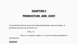
Chapter-3: Production and Costs, Introduction:, Production is the process by which inputs are transformed into ‘output’. Production is, carried out by producers or firms., A firm acquires different inputs like labour, machines, land, raw materials etc. It uses, these inputs to produce output. This output can be consumed by consumers, or used by other, firms for further production., In order to acquire inputs a firm has to pay for them. This is called the cost of, production. Once output has been produced, the firm sell it in the market and earns revenue., The difference between the revenue and cost is called the firm’s profit. We assume that the, objective of a firm is to earn the maximum profit that it can., , Production Function:, The production function of a firm is a relationship between inputs used and output, produced by the firm. For various quantities of inputs used, it gives the maximum quantity of, output that can be produced., A production function is defined for a given technology. It is the technological, knowledge that determines the maximum levels of output that can be produced using, different combinations of inputs., If the technology improves, the maximum levels of output obtainable for different input, combinations increase. We then have a new production function., The inputs that a firm uses in the production process are called factors of production., In order to produce output, a firm may require any number of different inputs. However, for, the time being, here we consider a firm that produces output using only two factors of, production – labour and capital., The production function, therefore, tells us the maximum quantity of output (q) that can, be produced by using different combinations of these two factors of productions- Labour (L), and Capital (K)., We may write the production function as:, q = ƒ(L,K), Where, L is labour and K is capital and q is the maximum output that can be produced.

Page 3 :
Isoquant:, An isoquant is the set of all possible combinations of the two inputs that yield the, same maximum possible level of output. Each isoquant represents a particular level of output, and is labelled with that amount of output., , In the above diagram, we place L on the X axis and K on the Y axis., , , We have three isoquants for the three output levels, namely q = q1, q = q2 and q = q3., , , , Two input combinations (L1, K2) and (L2, K1) give us the same level of output q1., , , , If we fix capital at K1 and increase labour to L3, output increases and we reach a higher, isoquant, q = q2., , , , When marginal products are positive, with greater amount of one input, the same level, of output can be produced only using lesser amount of the other., , , , Therefore, isoquants are negatively sloped., , The Short Run and The Long Run:, In the short run: at least one of the factor – labour or capital – cannot be varied, and therefore,, remains fixed. In order to vary the output level, the firm can vary only the other factor. The, factor that remains fixed is called the fixed factor whereas the other factor which the firm can, vary is called the variable factor., In the long run: all factors of production can be varied. A firm in order to produce different, levels of output in the long run may vary both the inputs simultaneously. So, in the long run,, there is no fixed factor., , , For different production processes, the long run periods may be different. It is not, advisable to define short run and long run in terms of say, days, months or years., , , , We define a period as long run or short run simply by looking at whether all the inputs, can be varied or not.

Page 4 :
Total Product, Average Product and Marginal Product:, Total Product (TP): It is the relationship between the variable input and output, keeping all, other inputs constant, is referred to as Total Product (TP) of the variable input. This is also, sometimes called total return or total physical product of the variable input., The total product is the total sum of the marginal product:, TPL=∑MPL, For example, TPL= 10+14+16+10+6+1, = 57, Average Product (AP): Average product is defined as the output per unit of variable input. It, is calculated as:, APL=, , TPL, L, , = 24/2 = 12, , Marginal Product (MP): Marginal product of an input is defined as the change in output per, unit of change in the input when all other inputs are held constant., MPL=, , Change in Output, Change in Input, , =, , ∆TPL, ∆L, , =, , 24-10, 2-1, , =14, , Or, MPL= (TP at L units) – (TP at L – 1 unit), Change in TP = 24 -10 = 14, Change in L = 1, Total Product, Marginal product and Average product, Labour, 0, 1, 2, 3, 4, 5, 6, , TP, , MP1, , AP1, , 0, 10, 24, 40, 50, 56, 57, , 10, 14, 16, 10, 6, 1, , 10, 12, 13.33, 12.5, 11.2, 9.5, , The Law of Diminishing Marginal Product:, The law of diminishing marginal product is that “the marginal product of a factor, input initially rises with its employment level. But after reaching a certain level of, employment, it starts falling”.

Page 5 :
From the above graph, placing labour on the X-axis and output on the Y-axis, we get, the curves as shown. TP, AP and MP curves are plotted., , , TP increases as labour input increases. But the rate at which it increases is not constant., , , , The rate at which TP increases, is shown by the MP., , , , Notice that the MP first increases and then begins to fall., , , , This tendency of the MP to first increase and then fall is called the law of variable, proportions., , Why does this happen?, Factor proportions represent the ratio in which the two inputs are combined to produce, output. As we hold one factor fixed and keep increasing the other, the factor proportions, change., Initially, as we increase the amount of the variable input, the factor proportions become, more and more suitable for the production and marginal product increases. But after a certain, level of employment, the production process becomes too crowded with the variable input., Each additional labour is now proportionally less. The marginal product begins to fall., , Shapes of Total Product, Marginal Product and Average Product Curves:, Total Product Curve (TPL):, We measure units of labour along the horizontal axis and output along the vertical axis., With L units of labour, the firm can at most produce q1 units of output., , Figure shows the shape of the total product curve for a, typical firm. When all other inputs are held constant, it, shows the different output levels obtainable from, different units of labour.

Page 6 :
Marginal Product (MPL) and Average Product (APL) curve:, According to the law of variable proportions, the marginal product of an input initially, rises and then after a certain level of employment, it starts falling. The MP curve therefore,, looks like an inverse ‘U’-shaped curve as in the figure., , , , For the first unit of the variable input, one can easily check that the MP and the AP are, same. Now as we increase the amount of input, the MP rises. AP being the average of, marginal products, also rises, but rises less than MP. Then, after a point, the MP starts, falling. However, as long as the value of MP remains higher than the value of the AP, the, AP continues to rise., , , , Once MP has fallen sufficiently, its value becomes less than the AP and the AP also starts, falling. So AP curve is also inverse ‘U’-shaped., , , , As long as the AP increases, it must be the case that MP is greater than AP. Otherwise, AP, cannot rise. Similarly, when AP falls, MP has to be less than AP. It, follows that MP curve, cuts AP curve from above at its maximum., , The following table gives the TP schedule of labour. Calculation of the corresponding Average, product and marginal product schedules., 0, 0, , TPL, L, L, 0, 1, 2, 3, 4, 5, , 15, 1, TPL, 0, 15, 35, 50, 40, 48, , 35, 2, , 50, 3, , MPL, 15, 20, 15, -10, 8, , 40, 4, , 48, 5, , APL, 15, 17.2, 16.66, 10, 9.6

Page 7 :
Returns to Scale:, The returns to scale can happen only in the long run as both the factors (Labour and, Capital) can be changed. One special case in the long run occurs when both factors are, increased by the same proportion, or factors are scaled up., Constant returns to scale (CRS): When a proportional increase in all inputs results in an, increase in output by the same proportion, the production function is said to display Constant, returns to scale (CRS)., Increasing Returns to Scale (IRS): When a proportional increase in all inputs results in an, increase in output by a larger proportion, the production function is said to display Increasing, Returns to Scale (IRS)., Decreasing Returns to Scale (DRS): DRS holds when a proportional increase in all inputs, results in an increase in output by a smaller proportion., , Cost Function:, The cost function describes the least cost of producing each level of output given prices, of factors of production and technology., Cobb-Douglas Production Function: Consider a production function, q = x1α x2β, Where, α and β are constants. The firm produces q amount of output using x 1 amount, of factor 1 and x2 amount of factor 2. This is called a Cobb-Douglas production function., , Short Run Costs:, Types of Short run costs are:, 1. Total Cost (TC) = Total Fixed Cost (TFC) + Total Variable Cost (TVC)., 2. Short Run Average Cost (SAC) = Average Fixed Cost (AFC) + Average Variable, Cost(AVC)., 3. Short Run Marginal Cost (SMC)., Various Concepts of Costs, Output, (units)(q), 0, 1, 2, 3, 4, 5, , TFC + TVC =, 20, 20, 20, 20, 20, 20, , 0, 10, 18, 24, 29, 33, , TC, 20, 30, 38, 44, 49, 53, , AFC + AVC =, 20, 10, 6.67, 5, 4, , 10, 9, 8, 7.25, 6.6, , SAC, 30, 19, 14.67, 12.25, 10.6, , SMC, 10, 8, 6, 5, 4

Page 8 :
, , Total Fixed Cost (TFC):, The cost that a firm incurs to employ these fixed inputs is called the total fixed cost, (TFC)., Example: Rent, salaries of the permanent employees, etc., Whatever amount of output the firm produces, this cost remains fixed for the firm., From the table: TFC = 20., , , , Total Variable Cost (TVC):, The cost that a firm incurs to employ these variable inputs is called the total variable, cost (TVC)., Example: Purchase of raw materials, fuel, etc., From the table: TVC = 10, , , , Total Cost (TC):, Adding the fixed and the variable costs, we get the total cost (TC) of a firm., TC = TFC + TVC, E.g.: TC = 20 + 10 = 30, , , , Average Fixed Cost (AFC):, It is the fixed cost per unit of output. In other words, it is average expenses incurred on, a single unit of output produced., AFC =, , 𝐓𝐅𝐂, 𝐪, , E.g.: AFC = 20/1 = 20, , , Average Variable Cost(AVC):, It is a variable cost for per unit of output. It can be calculated by dividing total variable, cost by the total units of output., AVC =, , 𝐓𝐕𝐂, 𝐪, , E.g.: AVC = 10/1 = 10, , , Short Run Average Cost (SAC):, It is the total cost per unit of output., SAC = AFC + AVC, E.g.: SAC= 20 + 10 = 30

Page 9 :
, , Short Run Marginal Cost (SMC):, It is defined as the change in total cost per unit of change in output., ∆TC, ∆q, , Change in Total Cost, =, Change in Output, , SMC=, , =, , 30-20, 1, , =10, , Long Run Costs:, In the long run, all inputs are variable. There are no fixed costs. The total cost and the, total variable cost therefore, coincide in the long run., Types of Long Run costs:, 1. Long run average cost (LRAC): It is defined as cost per unit of output., LRAC =, , 𝐓𝐂, 𝐪, , 2. Long run marginal cost (LRMC): It is the change in total cost per unit of change in, output., When output changes in discrete units, then, if we increase production from q1–1 to q1, units of output, the marginal cost of producing q1th unit will be measured as;, LRMC = (TC at q1 units) – (TC at q1 – 1 units), , Shapes of the Long Run Cost Curves:, IRS implies that if we increase all the inputs by a certain proportion, output increases, by more than that proportion. In other words, to increase output by a certain proportion, inputs, need to be increased by less than that proportion. With the input prices given, cost also increases, by a lesser proportion., DRS implies that if we want to increase the output by a certain proportion, inputs need, to be increased by more than that proportion. As a result, cost also increases by more than that, proportion. So, as long as DRS operates, the average cost must be rising as the firm increases, output., CRS implies a proportional increase in inputs resulting in a proportional increase in, output. So the average cost remains constant as long as CRS operates. It is argued that in a, typical firm IRS is observed at the initial level of production. This is then followed by the CRS, and then by the DRS. Accordingly, the LRAC curve is a ‘U’-shaped curve. Its downward, sloping part correspond to IRS and upward rising part corresponds to DRS. At the minimum, point of the LRAC curve, CRS is observed.

Page 10 :
For the first unit of output, both LRMC and LRAC are the same. Then, as output, increases, LRAC initially falls, and then, after a certain point, it rises. As long as average cost, is falling, marginal cost must be less than the average cost. When the average cost is rising,, marginal cost must be greater than the average cost. LRMC curve is therefore a ‘U’-shaped, curve. It cuts the LRAC curve from below at the minimum point of the LRAC., , Figure shows the shapes of the long run marginal cost and the long run average cost, curves for a typical firm., , , LRAC reaches its minimum at q1. To the left of q1, LRAC is falling and LRMC is, less than the LRAC curve., , , , To the right of q1, LRAC is rising and LRMC is higher than LRAC., , A firm’s SMC schedule is shown in the following table. TFC is Rs.100. Calculation of, TVC, TC, AVC and SAC schedules of the firm:, Q, , 0, , 1, , 2, , 3, , 4, , 5, , 6, , SMC, , -, , 500, , 300, , 200, , 300, , 500, , 800, , Q SMC TFC TVC=∑SMC TC=TFC+TVC AFC=TFC/Q AVC=TVC/Q SAC=AFC+AVC, 0, , -, , 100, , 0, , 100, , -, , -, , -, , 1, , 500, , 100, , 500, , 600, , 100, , 500, , 600, , 2, , 300, , 100, , 800, , 900, , 50, , 400, , 450, , 3, , 200, , 100, , 1000, , 1100, , 33.33, , 333.33, , 366.66, , 4, , 300, , 100, , 1300, , 1400, , 25, , 325, , 350, , 5, , 500, , 100, , 1800, , 1900, , 20, , 360, , 380, , 6, , 800, , 100, , 2600, , 2700, , 16.67, , 433.33, , 450, , ****