Page 1 :
B. Sc. DEGREE PROGRAMME, (2020 Admission onwards), , COPLEMENTARY MATHEMATICS, SECOND SEMESTER, COPLEMENTARY : MTS2C02 -, , MATHEMATICS-2, 4 hours/week, 3 Credits, 75 Marks [Int:15+Ext:60]
Page 2 :
SECOND SEMESTER, MTS2 C02:MATHEMATICS-2, 4 hours/week, , 3 Credits, , 75 Marks [Int:15+Ext:60], , Syllabus, Text (1), , Calculus I (2/e) : Jerrold Marsden & Alan Weinstein Springer-Verlag New, York Inc(1985) ISBN 0-387-90974-5, , Text (2), , Calculus II (2/e) : Jerrold Marsden & Alan Weinstein Springer-Verlag New, York Inc(1985) ISBN 0-387-90975-3, , Text (3), , Advanced Engineering Mathematics(6/e) : Dennis G Zill Jones & Bartlett, Learning, LLC(2018)ISBN: 978-1-284-10590-2, , Module- I, , Text (1) & (2), , 14 hrs, , 5.1: Polar coordinates and Trigonometry – Cartesian and polar coordinates, (Only representation of points in polar coordinates, relationship between Cartesian and, polar coordinates, converting from one system to another and regions represented by, inequalities in polar system are required), 5.3 : Inverse functions-inverse function test, inverse function rule, 5.6: Graphing in polar coordinates- Checking symmetry of graphs given in polar equation,, drawings, tangents to graph in polar coordinates, 8.3: Hyperbolic functions- hyperbolic sine, cosine, tan etc., derivatives, anti differentiation, formulas, 8.4: Inverse hyperbolic functions- inverse hyperbolic functions (their derivatives and anti, derivatives), 10.3: Arc length and surface area- Length of curves, Area of surface of revolution about x, and y axes, , Module- II, , Text (2), , 17 hrs, , 11.3: Improper integrals- integrals over unbounded intervals, comparison test, integrals of, unbounded functions, 11.4: Limit of sequences and Newton’s method ε-N definition, limit of powers,, comparison test, Newton’s method, 11.5: Numerical Integration- Riemann Sum, Trapezoidal Rule, Simpson’s Rule, , 82, , Page 84 of 100
Page 3 :
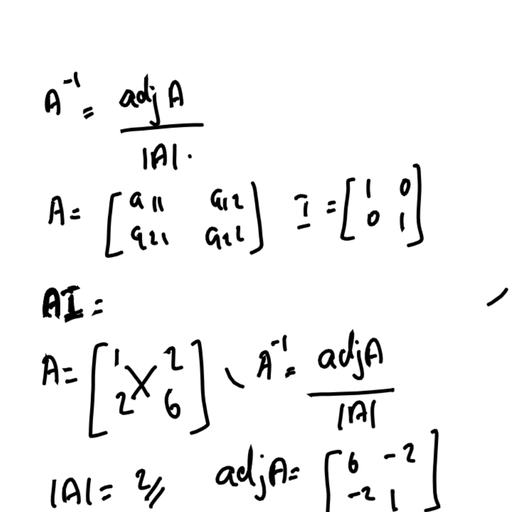
12.1: The sum of an infinite series- convergence of series, properties of limit of sequences, th, , (statements only), geometric series, algebraic rules for series, the i term test, 12.2: The comparison test and alternating series- comparison test, ratio comparison test,, alternating series, alternating series test, absolute and conditional convergence, , Text (3), , Module- III, , 19 hrs, , 7.6: Vector spaces – definition, examples , subspaces, basis, dimension, span, 7.7: Gram-Schmidt Orthogonalization Process- orthonormal bases for ℝ n, construction of, n, , orthonomal basis of ℝ, , 8.2: Systems of Linear Algebraic Equations- General form, solving systems, augmented, matrix, Elementary row operations, Elimination Methods- Gaussian elimination, Gauss–, Jordan elimination, row echelon form, reduced row echelon form, inconsistent system,, networks, homogeneous system, over and underdetermined system, 8.3: Rank of a Matrix- definition, row space, rank by row reduction, rank and linear system,, consistency of linear system, 8.4: Determinants- definition, cofactor (quick introduction), 8.5: Properties of determinant- properties, evaluation of determinant by row reducing to, triangular form, , Module- IV, , Text (3), , 14 hrs, , 8.6: Inverse of a Matrix – finding inverse, properties of inverse, adjoint method, row, operations method, using inverse to solve a linear system, 8.8: The eigenvalue problem- Definition, finding eigenvalues and eigenvectors, complex, eigenvalues, eigenvalues and singular matrices, eigenvalues of inverse, 8.9: Powers of Matrices- Cayley Hamilton theorem, finding the inverse, 8.10: Orthogonal Matrices- symmetric matrices and eigenvalues, inner product, criterion for, orthogonal matrix, construction of orthogonal matrix, 8.12:, Diagonalizationdiagonalizable, matrix-sufficient, diagonalizability of symmetric matrix, Quadratic Forms, , 83, , conditions,, , orthogonal, , Page 85 of 100
Page 4 :
References:, 1 Soo T Tan: Calculus Brooks/Cole, Cengage Learning(2010 )ISBN 0-534-46579-X, 2 Gilbert Strang: Calculus Wellesley Cambridge Press(1991)ISBN:0-9614088-2-0, 3, , Ron Larson. Bruce Edwards: Calculus(11/e) Cengage Learning(2018) ISBN: 978-1-33727534-7, , 4, , Robert A Adams & Christopher Essex : Calculus Single Variable (8/e) Pearson Education, Canada (2013) ISBN: 0321877403, , 5, , Joel Hass, Christopher Heil & Maurice D. Weir : Thomas’ Calculus(14/e), Pearson (2018) ISBN 0134438981, , 6, , Advanced Engineering Mathematics(7/e) Peter V O’Neil: Cengage, Learning(2012)ISBN: 978-1-111-42741-2, , 7, , Erwin Kreyszig: Advanced Engineering Mathematics(10/e) John Wiley & Sons(2011), ISBN: 978-0-470-45836-5, , 8, , 1Glyn James: Advanced Modern Engineering Mathematics(4/e) Pearson Education, Limited(2011) ISBN: 978-0-273-71923-6, , 84, , Page 86 of 100
Page 5 :
MODULE 1, Text (1) Calculus I (2/e) : Jerrold Marsden & Alan, Weinstein Springer-Verlag New York Inc(1985) ISBN, 0387909745, Text (2) Calculus II (2/e) : Jerrold Marsden & Alan, Weinstein Springer-Verlag New York Inc(1985) ISBN, 0387909753, Sections 5.1, 5.3, 5.6 - Text (1), 8.3, 8.4, 10.3 - Text (2)
Page 74 :
MODULE 2, Text (2) Calculus II (2/e) : Jerrold Marsden & Alan, Weinstein Springer-Verlag New York Inc(1985) ISBN, 0387909753, Sections 11.3-11.5, 12.1-12.2
Page 129 :
MODULE 3, Text (3) Advanced Engineering Mathematics(6/e) :, Dennis G Zill Jones & Bartlett Learning,, LLC(2018)ISBN: 9781284105902, Sections 7.6-7.7, 8.2-8.5
Page 130 :
63. Determine which of the following planes are perpendicular, , 43. ( 12 , 34 , � 12 ); 6i � 8j � 4k, 44. (�1, 1, 0); �i � j � k, , In Problems 45–50, find, if possible, an equation of a plane that, contains the given points., 45., 46., 47., 48., 49., 50., , (3, 5, 2), (2, 3, 1), (�1, �1, 4), (0, 1, 0), (0, 1, 1), (1, 3, �1), (0, 0, 0), (1, 1, 1), (3, 2, �1), (0, 0, 3), (0, �1, 0), (0, 0, 6), (1, 2, �1), (4, 3, 1), (7, 4, 3), (2, 1, 2), (4, 1, 0), (5, 0, �5), , In Problems 65–68, find parametric equations for the line of, intersection of the given planes., , In Problems 51–60, find an equation of the plane that satisfies, the given conditions., 51., 52., 53., 54., 55., 56., 57., 58., 59., 60., 61., , 62., , to the line x � 4 � 6t, y � 1 � 9t, z � 2 � 3t., (a) 4x � y � 2z � 1, (b) 2x � 3y � z � 4, (c) 10x � 15y � 5z � 2 (d) �4x � 6y � 2z � 9, 64. Determine which of the following planes are parallel to the, line (1 � x)/2 � (y � 2)/4 � z � 5., (a) x � y � 3z � 1, (b) 6x � 3y � 1, (c) x � 2y � 5z � 0, (d) �2x � y � 2z � 7, , Contains (2, 3, �5) and is parallel to x � y � 4z � 1, Contains the origin and is parallel to 5x � y � z � 6, Contains (3, 6, 12) and is parallel to the xy-plane, Contains (�7, �5, 18) and is perpendicular to the y-axis, Contains the lines x � 1 � 3t, y � 1 � t, z � 2 � t;, x � 4 � 4s, y � 2s, z � 3 � s, y�1, z25, x21, �, �, ;, Contains the lines, 2, �1, 6, r � �1, �1, 5� � t �1, 1, �3�, Contains the parallel lines x � 1 � t, y � 1 � 2t, z � 3 � t;, x � 3 � s, y � 2s, z � �2 � s, Contains the point (4, 0, �6) and the line x � 3t, y � 2t,, z � �2t, Contains (2, 4, 8) and is perpendicular to the line x � 10 � 3t,, y � 5 � t, z � 6 � 12 t, Contains (1, 1, 1) and is perpendicular to the line through, (2, 6, �3) and (1, 0, �2), Let �1 and �2 be planes with normal vectors n1 and n2,, respectively. �1 and �2 are orthogonal if n 1 and n2 are, orthogonal and parallel if n1 and n2 are parallel. Determine, which of the following planes are orthogonal and which, are parallel., (a) 2x � y � 3z � 1, (b) x � 2y � 2z � 9, (d) �5x � 2y � 4z � 0, (c) x � y � 32 z � 2, (e) �8x � 8y � 12z � 1 (f ) �2x � y � 3z � 5, Find parametric equations for the line that contains (�4, 1, 7), and is perpendicular to the plane �7x � 2y � 3z � 1., , 7.6, , 65. 5x � 4y � 9z � 8, , x � 4y � 3z � 4, 67. 4x � 2y � z � 1, x � y � 2z � 1, , x � 2y � z � 2, 3x � y � 2z � 1, 68. 2x � 5y � z � 0, y, �0, 66., , In Problems 69–72, find the point of intersection of the given, plane and line., 69., 70., 71., 72., , 2x � 3y � 2z � �7; x � 1 � 2t, y � 2 � t, z � �3t, x � y � 4z � 12; x � 3 � 2t, y � 1 � 6t, z � 2 � 12 t, x � y � z � 8; x � 1, y � 2, z � 1 � t, x � 3y � 2z � 0; x � 4 � t, y � 2 � t, z � 1 � 5t, , In Problems 73 and 74, find parametric equations for the line, through the indicated point that is parallel to the given planes., x � y � 4z � 2, 2x � y � z � 10; (5, 6, �12), 74. 2x �, z�0, �x � 3y � z � 1; (�3, 5, �1), 73., , In Problems 75 and 76, find an equation of the plane that contains the given line and is orthogonal to the indicated plane., 75. x � 4 � 3t, y � �t, z � 1 � 5t; x � y � z � 7, 76., , y�2, 22x, z28, �, �, ; 2x � 4y � z � 16 � 0, 3, 5, 2, , In Problems 77–82, graph the given equation., 77. 5x � 2y � z � 10, 79. �y � 3z � 6 � 0, 81. �x � 2y � z � 4, , 78. 3x � 2z � 9, 80. 3x � 4y � 2z � 12 � 0, 82. x � y � 1 � 0, , Vector Spaces, , INTRODUCTION In the preceding sections we were dealing with points and vectors in 2- and, , 3-space. Mathematicians in the nineteenth century, notably the English mathematicians Arthur, Cayley (1821–1895) and James Joseph Sylvester (1814–1897) and the Irish mathematician, William Rowan Hamilton (1805–1865), realized that the concepts of point and vector could, be generalized. A realization developed that vectors could be described, or defined, by analytic, rather than geometric properties. This was a truly significant breakthrough in the history of, mathematics. There is no need to stop with three dimensions; ordered quadruples �a1, a2, a3, a4�,, quintuples �a1, a2, a3, a4, a5�, and n-tuples �a1, a2, … , an� of real numbers can be thought of as, vectors just as well as ordered pairs �a1, a2� and ordered triples �a1, a2, a3�; the only difference, being that we lose our ability to visualize directed line segments or arrows in 4-dimensional,, 5-dimensional, or n-dimensional space., 7.6 Vector Spaces, , |, , 351
Page 131 :
n-Space In formal terms, a vector in n-space is any ordered n-tuple a � �a1, a2, … , an � of, real numbers called the components of a. The set of all vectors in n-space is denoted by R n. The, concepts of vector addition, scalar multiplication, equality, and so on, listed in Definition 7.2.1, carry over to R n in a natural way. For example, if a � �a1, a2, … , an � and b � �b1, b2, … , bn �,, then addition and scalar multiplication in n-space are defined by, a � b � �a1 � b1, a2 � b2, … , an � bn �, , ka � �ka1, ka2, … , kan �., , and, , (1), , The zero vector in R n is 0 � �0, 0, … , 0�. The notion of length or magnitude of a vector, a � �a1, a2, … , an� in n-space is just an extension of that concept in 2- and 3-space:, iai � "a 21 � a 22 � p � a 2n ., The length of a vector is also called its norm. A unit vector is one whose norm is 1. For a nonzero, vector a, the process of constructing a unit vector u by multiplying a by the reciprocal, 1, of its norm, that is, u �, a, is referred to as normalizing a. For example, if a � �3, 1, 2, �1�,, iai, then iai � "32 � 12 � 22 � (�1)2 � "15 and a unit vector is, u�, , 1, "15, , a� h, , 3, , ,, , 1, , ,, , 2, , "15 "15 "15, , ,�, , 1, "15, , i., , The standard inner product, also known as the Euclidean inner product or dot product,, of two n-vectors a � �a1, a2, … , an� and b � �b1, b2, … , bn� is the real number defined by, a b � �a1, a2, … , an� �b1, b2, … , bn� � a1b1 � a2b2 �, , � anbn., , (2), , Two nonzero vectors a and b in R n are said to be orthogonal if and only if a b � 0. For, example, a � �3, 4, 1, �6� and b � �1, 12 , 1, 1� are orthogonal in R 4 since a b � 3 1 � 4 12 �, 1 1 � (�6) 1 � 0., , Vector Space We can even go beyond the notion of a vector as an ordered n-tuple in Rn. A, , vector can be defined as anything we want it to be: an ordered n-tuple, a number, an array of numbers,, or even a function. But we are particularly interested in vectors that are elements in a special kind, of set called a vector space. Fundamental to the notion of vector space are two kinds of objects,, vectors and scalars, and two algebraic operations analogous to those given in (1). For a set of vectors we want to be able to add two vectors in this set and get another vector in the same set, and we, want to multiply a vector by a scalar and obtain a vector in the same set. To determine whether a, set of objects is a vector space depends on whether the set possesses these two algebraic operations, along with certain other properties. These properties, the axioms of a vector space, are given next., Definition 7.6.1, , Vector Space, , Let V be a set of elements on which two operations called vector addition and scalar multiplication, are defined. Then V is said to be a vector space if the following 10 properties are satisfied., Axioms for Vector Addition:, (i) If x and y are in V, then x � y is in V., (ii) For all x, y in V, x � y � y � x., (iii) For all x, y, z in V, x � (y � z) � (x � y) � z., (iv) There is a unique vector 0 in V such that, 0 � x � x � 0 � x., (v) For each x in V, there exists a vector �x such that, x � (�x) � (�x) � x � 0., Axioms for Scalar Multiplication:, (vi) If k is any scalar and x is in V, then kx is in V., (vii) k(x � y) � kx � ky, (viii) (k1 � k2)x � k1x � k2x, (ix) k1(k2x) � (k1k2)x, (x) 1x � x, , 352, , |, , CHAPTER 7 Vectors, , d commutative law, d associative law, d zero vector, d negative of a vector, , d distributive law, d distributive law
Page 132 :
In this brief introduction to abstract vectors we shall take the scalars in Definition 7.6.1 to be, real numbers. In this case V is referred to as a real vector space, although we shall not belabor this, term. When the scalars are allowed to be complex numbers we obtain a complex vector space., Since properties (i)–(viii) on page 352 are the prototypes for the axioms in Definition 7.6.1, it is, clear that R2 is a vector space. Moreover, since vectors in R3 and R n have these same properties,, we conclude that R3 and R n are also vector spaces. Axioms (i) and (vi) are called the closure, axioms and we say that a vector space V is closed under vector addition and scalar multiplication., Note, too, that concepts such as length and inner product are not part of the axiomatic structure, of a vector space., EXAMPLE 1, , Checking the Closure Axioms, , Determine whether the sets (a) V � {1} and (b) V � {0} under ordinary addition and multiplication by real numbers are vector spaces., SOLUTION (a) For this system consisting of one element, many of the axioms given in, Definition 7.6.1 are violated. In particular, axioms (i) and (vi) of closure are not satisfied., Neither the sum 1 � 1 � 2 nor the scalar multiple k � 1 � k, for k � 1, is in V. Hence V is, not a vector space., (b) In this case the closure axioms are satisfied since 0 � 0 � 0 and k � 0 � 0 for any real, number k. The commutative and associative axioms are satisfied since 0 � 0 � 0 � 0 and, 0 � (0 � 0) � (0 � 0) � 0. In this manner it is easy to verify that the remaining axioms are, also satisfied. Hence V is a vector space., The vector space V � {0} is often called the trivial or zero vector space., If this is your first experience with the notion of an abstract vector, then you are cautioned, to not take the names vector addition and scalar multiplication too literally. These operations, are defined and as such you must accept them at face value even though these operations may, not bear any resemblance to the usual understanding of ordinary addition and multiplication in,, say, R, R 2, R 3, or R n. For example, the addition of two vectors x and y could be x � y. With this, forewarning, consider the next example., EXAMPLE 2, , An Example of a Vector Space, , Consider the set V of positive real numbers. If x and y denote positive real numbers, then we, write vectors in V as x � x and y � y. Now, addition of vectors is defined by, x � y � xy, and scalar multiplication is defined by, kx � x k., Determine whether V is a vector space., SOLUTION We shall go through all ten axioms in Definition 7.6.1., For x � x � 0 and y � y � 0, x � y � xy � 0. Thus, the sum x � y is in V; V is, closed under addition., (ii) Since multiplication of positive real numbers is commutative, we have for all, x � x and y � y in V, x � y � xy � yx � y � x. Thus, addition is commutative., (iii) For all x � x, y � y, z � z in V,, , (i), , x � (y � z) � x(yz) � (xy)z � (x � y) � z., Thus, addition is associative., (iv) Since 1 � x � 1x � x � x and x � 1 � x1 � x � x, the zero vector 0 is 1 � 1., 1, (v) If we define �x � , then, x, 1, 1, x � (�x) � x � 1 � 1 � 0 and (�x) � x � x � 1 � 1 � 0., x, x, Therefore, the negative of a vector is its reciprocal., 7.6 Vector Spaces |, , 353
Page 133 :
(vi) If k is any scalar and x � x � 0 is any vector, then k x � x k � 0. Hence V is closed, under scalar multiplication., (vii) If k is any scalar, then, k(x � y) � (xy)k � xk yk � kx � ky., (viii) For scalars k1 and k2,, (k1 � k2)x � x (k1 � k2) � x k1 x k2 � k1x � k2x., (ix) For scalars k1 and k2,, k1(k2x) � (x k2)k1 � x k1 k2 � (k1k2)x., (x) 1x � x1 � x � x., Since all the axioms of Definition 7.6.1 are satisfied, we conclude that V is a vector space., Here are some important vector spaces—we have mentioned some of these previously. The, operations of vector addition and scalar multiplication are the usual operations associated with, the set., •, •, •, •, •, •, •, •, •, •, , The set R of real numbers, The set R2 of ordered pairs, The set R3 of ordered triples, The set R n of ordered n-tuples, The set Pn of polynomials of degree less than or equal to n, The set P of all polynomials, The set of real-valued functions f defined on the entire real line, The set C[a, b] of real-valued functions f continuous on the closed interval [a, b], The set C(�q , q ) of real-valued functions f continuous on the entire real line, The set C n [a, b] of all real-valued functions f for which f, f �, f �, … , f (n) exist and are, continuous on the closed interval [a, b], , Subspace It may happen that a subset of vectors W of a vector space V is itself a vector, , space., , Definition 7.6.2, , Subspace, , If a subset W of a vector space V is itself a vector space under the operations of vector addition, and scalar multiplication defined on V, then W is called a subspace of V., Every vector space V has at least two subspaces: V itself and the zero subspace {0}; {0} is a, subspace since the zero vector must be an element in every vector space., To show that a subset W of a vector space V is a subspace, it is not necessary to demonstrate, that all ten axioms of Definition 7.6.1 are satisfied. Since all the vectors in W are also in V, these, vectors must satisfy axioms such as (ii) and (iii). In other words, W inherits most of the properties of a vector space from V. As the next theorem indicates, we need only check the two closure, axioms to demonstrate that a subset W is a subspace of V., Theorem 7.6.1, , Criteria for a Subspace, , A nonempty subset W of a vector space V is a subspace of V if and only if W is closed under, vector addition and scalar multiplication defined on V:, (i) If x and y are in W, then x � y is in W., (ii) If x is in W and k is any scalar, then k x is in W., , EXAMPLE 3, , A Subspace, , Suppose f and g are continuous real-valued functions defined on the entire real line. Then we, know from calculus that f � g and k f, for any real number k, are continuous and real-valued, functions. From this we can conclude that C(� q , q ) is a subspace of the vector space of, real-valued functions defined on the entire real line., 354, , |, , CHAPTER 7 Vectors
Page 134 :
EXAMPLE 4, , A Subspace, , The set Pn of polynomials of degree less than or equal to n is a subspace of C(� q , q ), the, set of real-valued functions continuous on the entire real line., It is always a good idea to have concrete visualizations of vector spaces and subspaces. The, subspaces of the vector space R3 of three-dimensional vectors can be easily visualized by thinking of a vector as a point (a1, a2, a3). Of course, {0} and R 3 itself are subspaces; other subspaces, are all lines passing through the origin, and all planes passing through the origin. The lines and, planes must pass through the origin since the zero vector 0 � (0, 0, 0) must be an element in, each subspace., Similar to Definition 3.1.1 we can define linearly independent vectors., Definition 7.6.3, , Linear Independence, , A set of vectors {x1, x2, … , xn} is said to be linearly independent if the only constants satisfying the equation, k1x1 � k2x2 �, , (3), , � kn x n � 0, , are k1 � k2 �, � kn � 0. If the set of vectors is not linearly independent, then it is said to, be linearly dependent., In R3, the vectors i � �1, 0, 0�, j � �0, 1, 0�, and k � �0, 0, 1� are linearly independent since, the equation k1i � k2 j � k3k � 0 is the same as, k1�1, 0, 0� � k2�0, 1, 0� � k3�0, 0, 1� � �0, 0, 0�, , or, , �k1, k2, k3� � �0, 0, 0�., , By equality of vectors, (iii) of Definition 7.2.1, we conclude that k1 � 0, k2 � 0, and k3 � 0. In, Definition 7.6.3, linear dependence means that there are constants k1, k2, … , kn not all zero such, that k1x1 � k2x2 � � knxn � 0. For example, in R3 the vectors a � �1, 1, 1�, b � �2, �1, 4�,, and c � �5, 2, 7� are linearly dependent since (3) is satisfied when k1 � 3, k2 � 1, and k3 � �1:, 3�1, 1, 1� � �2, �1, 4� � �5, 2, 7� � �0, 0, 0�, , or, , 3a � b � c � 0., , We observe that two vectors are linearly independent if neither is a constant multiple of the, other., , Basis Any vector in R 3 can be written as a linear combination of the linearly independent, , vectors i, j, and k. In Section 7.2, we said that these vectors form a basis for the system of threedimensional vectors., Definition 7.6.4, , Basis for a Vector Space, , Consider a set of vectors B � {x1, x2, … , xn} in a vector space V. If the set B is linearly, independent and if every vector in V can be expressed as a linear combination of these vectors,, then B is said to be a basis for V., , Standard Bases Although we cannot prove it in this course, every vector space has a basis., The vector space Pn of all polynomials of degree less than or equal to n has the basis {1, x, x2, … , xn}, since any vector (polynomial) p(x) of degree n or less can be written as the linear combination, p(x) � cnxn � � c2x2 � c1x � c0. A vector space may have many bases. We mentioned previously the set of vectors {i, j, k} is a basis for R 3. But it can be proved that {u1, u2, u3}, where, u1 � �1, 0, 0�,, , u2 � �1, 1, 0�,, , u3 � �1, 1, 1�, , is a linearly independent set (see Problem 23 in Exercises 7.6) and, furthermore, every vector, a � �a1, a2, a3� can be expressed as a linear combination a � c1u1 � c2u2 � c3u3. Hence, the set, of vectors {u1, u2, u3} is another basis for R3. Indeed, any set of three linearly independent vectors is a basis for that space. However, as mentioned in Section 7.2, the set {i, j, k} is referred to, as the standard basis for R3. The standard basis for the space Pn is {1, x, x2, … , xn}. For the, 7.6 Vector Spaces, , |, , 355
Page 135 :
vector space R n, the standard basis consists of the n vectors, e1 � �1, 0, 0, … , 0�, e2 � �0, 1, 0, … , 0�, … , en � �0, 0, 0, … , 1�., , (4), , If B is a basis for a vector space V, then for every vector v in V there exist scalars ci, i � 1, 2, . . . , n, such that, v � c1x2 � c2x2 � p � cnxn., (5), Read the last sentence, several times., , The scalars ci , i � 1, 2, … , n, in the linear combination (5) are called the coordinates of v relative, to the basis B. In R n, the n-tuple notation �a1, a2, … , an� for a vector a means that real numbers, a1, a2, … , an are the coordinates of a relative to the standard basis with ei’s in the precise order, given in (4)., , Dimension If a vector space V has a basis B consisting of n vectors, then it can be proved, that every basis for that space must contain n vectors. This leads to the next definition., Definition 7.6.5, , Dimension of a Vector Space, , The number of vectors in a basis B for a vector space V is said to be the dimension of the, space., , Dimensions of Some Vector Spaces, , EXAMPLE 5, , (a) In agreement with our intuition, the dimensions of the vector spaces R, R 2, R 3, and R n, are, in turn, 1, 2, 3, and n., (b) Since there are n � 1 vectors in the standard basis B � {1, x, x2, … , x n}, the dimension, of the vector space Pn of polynomials of degree less than or equal to n is n � 1., (c) The zero vector space {0} is given special consideration. This space contains only 0, and since {0} is a linearly dependent set, it is not a basis. In this case it is customary to take, the empty set as the basis and to define the dimension of {0} as zero., If the basis of a vector space V contains a finite number of vectors, then we say that the vector, space is finite dimensional; otherwise it is infinite dimensional. The function space C n (I ) of n, times continuously differentiable functions on an interval I is an example of an infinite-dimensional, vector space., , Linear Differential Equations Consider the homogeneous linear nth-order differential, , equation, , an(x), , d ny, d n 2 1y, dy, �, a, (x), � p � a1(x), � a0(x)y � 0, n21, n, n21, dx, dx, dx, , (6), , on an interval I on which the coefficients are continuous and an(x) � 0 for every x in the interval., A solution y1 of (6) is necessarily a vector in the vector space C n (I). In addition, we know from, the theory examined in Section 3.1 that if y1 and y2 are solutions of (6), then the sum y1 � y2 and, any constant multiple ky1 are also solutions. Since the solution set is closed under addition and, scalar multiplication, it follows from Theorem 7.6.1 that the solution set of (6) is a subspace of, C n (I ). Hence the solution set of (6) deserves to be called the solution space of the differential, equation. We also know that if {y1, y2, … , yn} is a linearly independent set of solutions of (6),, then its general solution of the differential equation is the linear combination, y � c1y1(x) � c2 y2(x) � p � cn yn(x)., Recall that any solution of the equation can be found from this general solution by specialization, of the constants c1, c2, … , cn. Therefore, the linearly independent set of solutions {y1, y2, … , yn}, is a basis for the solution space. The dimension of this solution space is n., EXAMPLE 6, , Dimension of a Solution Space, , The general solution of the homogeneous linear second-order differential equation y� � 25y � 0, is y � c1 cos 5x � c2 sin 5x. A basis for the solution space consists of the linearly independent, vectors {cos 5x, sin 5x}. The solution space is two-dimensional., 356, , |, , CHAPTER 7 Vectors
Page 136 :
The set of solutions of a nonhomogeneous linear differential equation is not a vector space. Several, axioms of a vector space are not satisfied; most notably the set of solutions does not contain a zero, vector. In other words, y � 0 is not a solution of a nonhomogeneous linear differential equation., , Span If S denotes any set of vectors {x1, x2, … , xn} in a vector space V, then the set of all, linear combinations of the vectors x1, x2, … , xn in S,, {k1x1 � k2x2 � p � knxn},, where the ki, i � 1, 2, … , n are scalars, is called the span of the vectors and written Span(S), or Span(x1, x2, … , xn). It is left as an exercise to show that Span(S) is a subspace of the vector, space V. See Problem 33 in Exercises 7.6. Span(S) is said to be a subspace spanned by the vectors, x1, x2, … , xn. If V � Span(S), then we say that S is a spanning set for the vector space V, or that, S spans V. For example, each of the three sets, {i, j, k},, , {i, i � j, i � j � k},, , and, , {i, j, k, i � j, i � j � k}, , are spanning sets for the vector space R 3. But note that the first two sets are linearly independent,, whereas the third set is dependent. With these new concepts we can rephrase Definitions 7.6.4, and 7.6.5 in the following manner:, A set S of vectors {x1, x2, … , xn} in a vector space V is a basis for V if S is linearly, independent and is a spanning set for V. The number of vectors in this spanning set S is, the dimension of the space V., , REMARKS, (i) Suppose V is an arbitrary real vector space. If there is an inner product defined on V it need not, look at all like the standard or Euclidean inner product defined on Rn. In Chapter 12 we will work, with an inner product that is a definite integral. We shall denote an inner product that is not the, Euclidean inner product by the symbol (u, v). See Problems 30, 31, and 38(b) in Exercises 7.6., (ii) A vector space V on which an inner product has been defined is called an inner product, space. A vector space V can have more than one inner product defined on it. For example, a, non-Euclidean inner product defined on R2 is (u, v) � u1v1 � 4u2v2, where u � �u1, u2� and, v � �v1, v2�. See Problems 37 and 38(a) in Exercises 7.6., (iii) A lot of our work in the later chapters in this text takes place in an infinite-dimensional, vector space. As such, we need to extend the definition of linear independence of a finite set, of vectors S � {x1, x2, … , xn} given in Definition 7.6.3 to an infinite set:, An infinite set of vectors S � {x1, x2, …} is said to be linearly independent if every, finite subset of the set S is linearly independent. If the set S is not linearly independent,, then it is linearly dependent., We note that if S contains a linearly dependent subset, then the entire set S is linearly dependent., The vector space P of all polynomials has the standard basis B � {1, x, x 2, …}. The infinite, set B is linearly independent. P is another example of an infinite-dimensional vector space., , 7.6, , Exercises, , Answers to selected odd-numbered problems begin on page ANS-15., , In Problems 1–10, determine whether the given set is a vector, space. If not, give at least one axiom that is not satisfied. Unless, stated to the contrary, assume that vector addition and scalar, multiplication are the ordinary operations defined on that set., 1. The set of vectors �a1, a2�, where a1 � 0, a2 � 0, 2. The set of vectors �a1, a2�, where a2 � 3a1 � 1, 3. The set of vectors �a1, a2�, scalar multiplication defined by, , k�a1, a2� � �ka1, 0�, , 4. The set of vectors �a1, a2�, where a1 � a2 � 0, 5. The set of vectors �a1, a2, 0�, 6. The set of vectors �a1, a2�, addition and scalar multiplication, , defined by, , �a1, a2� � �b1, b2� � �a1 � b1 � 1, a2 � b2 � 1�, k�a1, a2� � �ka1 � k � 1, ka2 � k � 1�, 7. The set of real numbers, addition defined by x � y � x � y, , 7.6 Vector Spaces, , |, , 357
Page 137 :
8. The set of complex numbers a � bi, where i 2 � �1, addition, , and scalar multiplication defined by, k(a � bi) � ka � kbi, k a real number, , a, , a11, a21, , a12, b11, b � a, a22, b21, ka, , a12, b , addition and, a22, , b12, a12 � b12, b � a, b22, a22 � b22, a12, ka11, b � a, a22, ka21, , a11, a21, , x, is a vector in C[0, 3] but, x 2 � 4x � 3, not a vector in C[�3, 0]., , 29. Explain why f (x) �, , (a1 � b1i) � (a2 � b2i) � (a1 � a2) � (b1 � b2)i, a11, 9. The set of arrays of real numbers a, a21, scalar multiplication defined by, , 28. 1, (x � 1), (x � 1)2, x 2 in P2, , a11 � b11, b, a21 � b21, , ka12, b, ka22, , 10. The set of all polynomials of degree 2, , In Problems 11–16, determine whether the given set is a, subspace of the vector space C(�q , q )., , 30. A vector space V on which a dot or inner product has been, , defined is called an inner product space. An inner product, for the vector space C[a, b] is given by, ( f, g) �, , 13. All nonnegative functions f, 14. All functions f such that f (�x) � f (x), 15. All differentiable functions f, 16. All functions f of the form f (x) � c1ex � c2xex, , In Problems 17–20, determine whether the given set is, a subspace of the indicated vector space., 17. Polynomials of the form p(x) � c3x3 � c1x; P3, 18. Polynomials p that are divisible by x � 2; P2, , In C[0, 2p] compute (x, sin x)., 31. The norm of a vector in an inner product space is defined in, terms of the inner product. For the inner product given in, Problem 30, the norm of a vector is given by i f i � !( f, f )., In C[0, 2p] compute ixi and isin xi., 32. Find a basis for the solution space of, d 4y, d 3y, d 2y, 2, 2, �, 10, � 0., dx 4, dx 3, dx 2, 33. Let {x1, x2, … , xn} be any set of vectors in a vector space V., , Show that Span(x1, x2, … , xn) is a subspace of V., , Discussion Problems, 34. Discuss: Is R 2 a subspace of R 3? Are R 2 and R 3 subspaces, , of R 4?, 35. In Problem 9, you should have proved that the set M22 of, 2 2 arrays of real numbers, , 19. All unit vectors; R3, 20. Functions f such that, , eba, , S � {(x, y, z) Z x � at, y � bt, z � ct, a, b, c real numbers}., With addition and scalar multiplication the same as for vectors, �x, y, z �, show that S is a subspace of R 3., 22. In 3-space, a plane through the origin can be written as, S � {(x, y, z ) | ax � by � cz � 0, a, b, c real numbers}. Show, that S is a subspace of R3., 23. The vectors u1 � �1, 0, 0�, u2 � �1, 1, 0�, and u3 � �1, 1, 1�, form a basis for the vector space R 3., (a) Show that u1, u2, and u3 are linearly independent., (b) Express the vector a � �3, �4, 8� as a linear combination, of u1, u2, and u3., 24. The vectors p1(x) � x � 1, p2(x) � x � 1 form a basis for the, vector space P1., (a) Show that p1(x) and p2(x) are linearly independent., (b) Express the vector p(x) � 5x � 2 as a linear combination, of p1(x) and p2(x)., In Problems 25–28, determine whether the given vectors are, linearly independent or linearly dependent., 25. �4, �8�, ��6, 12� in R 2, 26. �1, 1�, �0, 1�, �2, 5� in R 2, 27. 1, (x � 1), (x � 1)2 in P2, , 358, , |, , M22 � e a, , f(x) dx � 0; C[a, b], , 21. In 3-space, a line through the origin can be written as, , CHAPTER 7 Vectors, , f (x)g(x) dx., , a, , 11. All functions f such that f (1) � 0, 12. All functions f such that f (0) � 1, , #, , b, , a11, a21, , a12, b f,, a22, , or matrices, is a vector space with vector addition and scalar, multiplication defined in that problem. Find a basis for M22., What is the dimension of M22?, 36. Consider a finite orthogonal set of nonzero vectors, {v1, v2, … , vk} in R n. Discuss: Is this set linearly independent, or linearly dependent?, 37. If u, v, and w are vectors in a vector space V, then the axioms, of an inner product (u, v) are, (i), (ii), (iii), (iv), , (u, v) � (v, u), (k u, v) � k(u, v), k a scalar, (u, u) � 0 if u � 0 and (u, u) � 0 if u � 0, (u, v � w) � (u, v) � (u, w)., , Show that (u, v) � u1v1 � 4u2v2, where u � �u1, u2� and, v � �v1, v2�, is an inner product on R2., 38. (a) Find a pair of nonzero vectors u and v in R2 that are not, , orthogonal with respect to the standard or Euclidean inner, product u v, but are orthogonal with respect to the inner, product (u, v) in Problem 37., (b) Find a pair of nonzero functions f and g in C[0, 2p] that, are orthogonal with respect to the inner product ( f, g), given in Problem 30.
Page 138 :
7.7, , Gram–Schmidt Orthogonalization Process, , INTRODUCTION In Section 7.6 we saw that a vector space V can have many different bases., Recall, the defining characteristics of any basis B � {x1, x2, … , xn} of a vector space V is that, , • the set B is linearly independent, and, • the set B spans the space., In this context the word span means that every vector in the space can be expressed as a linear, combination of the vectors x1, x2, … , xn. For example, every vector u in R n can be written as a, linear combination of the vectors in the standard basis B � {e1, e2, … , en}, where, e1 � �1, 0, 0, … , 0�,, , e2 � �0, 1, 0, … , 0�,, , …,, , en � �0, 0, 0, … , 1�., , This standard basis B � {e1, e2, … , en} is also an example of an orthonormal basis; that is, the, ei , i � 1, 2, … , n are mutually orthogonal and are unit vectors; that is,, ei � ej � 0, i � j, , i ei i � 1, i � 1, 2, … , n., , and, , In this section we focus on orthonormal bases for R n and examine a procedure whereby we, can transform or convert any basis B of R n into an orthonormal basis., , Orthonormal Basis for R 3, , EXAMPLE 1, , The set of three vectors, w1 � h, , 1, , ,, , 1, , ,, , 1, , "3 "3 "3, , i, w2 � h�, , 2, , ,, , 1, , ,, , 1, , "6 "6 "6, , i, w3 � h0 ,, , 1, "2, , ,�, , 1, "2, , i, , (1), , is linearly independent and spans the space R 3. Hence B � {w1, w2, w3} is a basis for R 3., Using the standard inner product or dot product defined on R 3, observe, w1 � w2 � 0, w1 � w3 � 0, w2 � w3 � 0,, , and, , i w1 i � 1, i w2 i � 1, i w3 i � 1., , Hence B is an orthonormal basis., A basis B for R n need not be orthogonal nor do the basis vectors need to be unit vectors. In, fact, any linearly independent set of n vectors can serve as a basis for the n-dimensional vector, space R n. For example, it is a straightforward task to show that the vectors, u1 � �1, 0, 0�,, , u2 � �1, 1, 0�,, , u3 � �1, 1, 1�, , in R 3 are linearly independent and hence B � {u1, u2, u3} is a basis for R 3. Note that B is not an, orthogonal basis., Generally, an orthonormal basis for a vector space V turns out to be the most convenient basis, for V. One of the advantages that an orthonormal basis has over any other basis for R n is the, comparative ease with which we can obtain the coordinates of a vector u relative to, that basis., Theorem 7.7.1, , Coordinates Relative to an Orthonormal Basis, , Suppose B � {w1, w2, … , wn} is an orthonormal basis for R n. If u is any vector in R n, then, u � (u � w1)w1 � (u � w2)w2 � p � (u � wn )wn., , PROOF: The vector u is in R n and so it is an element of the set Span(B). In other words, there, , exist real scalars ki, i � 1, 2, … , n such that u can be expressed as the linear combination, u � k1w1 � k2w2 � p � knwn., 7.7 Gram–Schmidt Orthogonalization Process |, , 359
Page 139 :
The scalars ki are the coordinates of u relative to the basis B. These coordinates can be found by, taking the dot product of u with each of the basis vectors:, u wi � (k1w1 � k2w2 � p � knwn) wi � k1(w1 wi) � k2(w2 wi) � p � kn(wn wi). (2), Since B is orthonormal, wi is orthogonal to all vectors in B with the exception of wi itself., That is, wi wj � 0, i � j and wi wi � i wi i 2 � 1. Hence from (2), we obtain ki � (u wi), for i � 1, 2, … , n., , Coordinates of a Vector in R 3, , EXAMPLE 2, , Find the coordinates of the vector u � � 3, �2, 9� relative to the orthonormal basis B for R 3, given in (1) of Example 1. Write u in terms of the basis B., SOLUTION From Theorem 7.7.1, the coordinates of u relative to the basis B in (1) of Example 1, are simply, u w1 �, , 10, "3, , , u w2 �, , 1, "6, , , and u w3 � �, , 11, , ., , "2, , Hence we can write, u�, , u2, , 10, "3, , u1, (a) Linearly independent vectors u1 and u2, , u2, , "6, , w2 2, , 11, "2, , w3 ., , Gram–Schmidt Orthogonalization Process The procedure known as the Gram–, Schmidt orthogonalization process is a straightforward algorithm for generating an orthogonal, basis B � {v1, v2, … , vn} from any given basis B � {u1, u2, … , un} for R n. We then produce an, orthonormal basis B� � {w1, w2, … , wn} by normalizing the vectors in the orthogonal basis B ., The key idea in the orthogonalization process is vector projection, and so we suggest that you, review that concept in Section 7.3. Also, for the sake of gaining some geometric insight into the, process, we shall begin in R 2 and R 3., process for R n is a sequence of steps; at each step we construct a vector vi that is orthogonal to, the vector in the preceding step. The transformation of a basis B � {u1, u2} for R 2 into an orthogonal basis B � {v1, v2} consists of two steps. See FIGURE 7.7.1(a). The first step is simple,, we merely choose one of the vectors in B, say, u1, and rename it v1. Next, as shown in Figure, 7.7.1(b), we project the remaining vector u2 in B onto the vector v1 and define a second vector, u 2 v1, bv . As seen in, to be v2 � u2 � proj v1 u2. Recall from (12) of Section 7.3 that proj v1 u2 � a, v1 v1 1, Figure 7.7.1(c), the vectors, , (b) Projection of u2 onto v1, , u2, v2 = u2 – projv u2, 1, , projv1u2, , 1, , Constructing an Orthogonal Basis for R 2 The Gram–Schmidt orthogonalization, , v1 = u1, , projv1u2, , w1 �, , v1 � u 1, , v1 = u1, , u 2 v1, v2 � u 2 2 a, bv, v1 v1 1, , (c) v1 and v2 are orthogonal, , FIGURE 7.7.1 The orthogonal vectors v1, and v2 are defined in terms of u1 and u2, , (3), , are orthogonal. If you are not convinced of this, we suggest you verify the orthogonality of v1, and v2 by demonstrating that v1 v2 � 0., EXAMPLE 3, , Gram–Schmidt Process in R 2, , The set B � {u1, u2}, where u1 � �3, 1�, u2 � �1, 1�, is a basis for R 2. Transform B into an, orthonormal basis B � � {w1, w2}., SOLUTION We choose v1 as u1: v1 � �3, 1�. Then from the second equation in (3), with, u2 v1 � 4 and v1 v1 � 10, we obtain, v2 � k1, 1l 2, 360, , |, , CHAPTER 7 Vectors, , 4, 1 3, k3, 1l � h� , i., 10, 5 5
Page 142 :
REMARKS, Although we have focused on R n in the foregoing discussion, the orthogonalization process, summarized in (7) of Theorem 7.7.2 holds in all vector spaces V on which an inner product, (u, v) is defined. In this case, we replace the symbol Rn in (7) with the words “an inner product, space V ” and each dot product symbol u � v with (u, v). See Problems 17 and 18 in Exercises 7.7., , Exercises, , 7.7, , Answers to selected odd-numbered problems begin on page ANS-16., , In Problems 1 and 2, verify that the basis B for the given vector, space is orthonormal. Use Theorem 7.7.1 to find the coordinates, of the vector u relative to the basis B. Then write u as a linear, combination of the basis vectors., 1. B � e h, 2. B � e h, , h�, , 2, , ,, , 5, 12 5, 12, , i, h , � i f ,, 13 13, 13, 13, 1, , 1, , 1, , R 2; u � k4 , 2l, 1, , 1, , ,, ,�, i, h0 , �, ,�, i,, "3 "3, "3, "2, "2, 1, , ,�, , "6 "6, , 1, "6, , 15. u1 � �1, �1, 1, �1�, u2 � �1, 3, 0, 1�, 16. u1 � �4, 0, 2, �1�, u2 � �2, 1, �1, 1�, u3 � �1, 1, �1, 0�, , In Problems 17 and 18, an inner product defined on the vector, space P2 of all polynomials of degree less than or equal to 2, is, given by, , i r , R 3; u � k5 , �1 , 6l, , In Problems 3 and 4, verify that the basis B for the given vector, space is orthogonal. Use Theorem 7.7.1 as an aid in finding the, coordinates of the vector u relative to the basis B. Then write, u as a linear combination of the basis vectors., 3. B � {�1, 0, 1�, �0, 1, 0�, ��1, 0, 1�, R3;, , u � �10, 7, �13�, , 4. B � {�2, 1, �2, 0�, �1, 2, 2, 1�, �3, �4, 1, 3�, �5, �2, 4, �9�}, R4;, , u � �1, 2, 4, 3�, , In Problems 5�8, use the Gram–Schmidt orthogonalization, process (3) to transform the given basis B � {u1, u2} for R2 into, an orthogonal basis B� � {v1, v2}. Then form an orthonormal, basis B� � {w1, w2}., (a) First construct B� using v1, u1., (b) Then construct B� using v1, u2., (c) Sketch B and each basis B�., 5. B � {��3, 2�, ��1, �1�} 6. B � {��3, 4�, ��1, 0�}, 7. B � {�1, 1�, �1, 0�}, 8. B � {�5, 7�, �1, �2�}, , In Problems 9–12, use the Gram–Schmidt orthogonalization, process (4) to transform the given basis B � {u1, u2, u3} for R3, into an orthogonal basis B� � {v1, v2, v3}. Then form an orthonormal basis B� � {w1, w2, w3}., 9., 10., 11., 12., , In Problems 15 and 16, the given vectors span a subspace W, of R 4. Use the Gram–Schmidt orthogonalization process to, construct an orthonormal basis for the subspace., , B � {�1, 1, 0�, �1, 2, 2�, �2, 2, 1�}, B � {��3, 1, 1�, �1, 1, 0�, ��1, 4, 1�}, B � {� 12 , 12 , 1�, ��1, 1, � 12 �, ��1, 12 , 1�}, B � {�1, 1, 1�, �9, �1, 1�, ��1, 4, �2�}, , In Problems 13 and 14, the given vectors span a subspace W, of R 3. Use the Gram–Schmidt orthogonalization process to, construct an orthonormal basis for the subspace., 13. u1 � �1, 5, 2�, u2 � ��2, 1, 1�, 14. u1 � �1, 2, 3�, u2 � �3, 4, 1�, , ( p, q) �, , #, , 1, , p(x) q(x) dx., , �1, , Use the Gram–Schmidt orthogonalization process to transform, the given basis B for P2 into an orthogonal basis B�., 17. B � {1, x, x2}, 18. B � {x2 � x, x2 � 1, 1 � x2}, , For the inner product (p, q) defined on P2 in Problems 17, and 18, the norm ip(x)i of a polynomial p is defined by, ip(x)i2 � ( p, p) �, , #, , 1, , p2(x) dx., , �1, , Use this norm in Problems 19 and 20., 19. Construct an orthonormal basis B� from B� obtained in, , Problem 17., 20. Construct an orthonormal basis B� from B� obtained in, , Problem 18., In Problems 21 and 22, let p(x) � 9x2 � 6x � 5 be a vector, in P2. Use Theorem 7.7.1 and the indicated orthonormal basis B�, to find the coordinates p(x) relative to B�. Then write p(x) as a, linear combination of the basis vectors., 21. B� in Problem 19, , 22. B� in Problem 20, , Discussion Problem, 23. The set of vectors {u1, u2, u3}, where, , u1 � �1, 1, 3�, u2 � � 1, 4, 1�, and u3 � � 1, 10, �3�,, is linearly dependent in R3 since u3 � �2u1 � 3u2. Discuss, what you would expect when the Gram–Schmidt process in (4), is applied to these vectors. Then carry out the orthogonalization, process., 7.7 Gram–Schmidt Orthogonalization Process |, , 363
Page 143 :
Chapter in Review, , 7, , Answers to selected odd-numbered problems begin on page ANS-16., , Answer Problems 1–30 without referring back to the text. Fill in, the blank or answer true/false., , 29. The distance from the plane y � �5 to the point (4, �3, 1), , 1. The vectors ��4, �6, 10� and ��10, �15, 25� are parallel., , 30. The vectors �1, 3, c� and ��2, �6, 5� are parallel for c � _____, , 2., 3., 4., 5., 6., 7., 8., 9., 10., 11., 12., 13., 14., 15., 16., 17., 18., 19., 20., 21., 22., 23., 24., 25., 26., 27., 28., , _____, In 3-space, any three distinct points determine a plane., _____, The line x � 1 � 5t, y � 1 � 2t, z � 4 � t and the plane, 2x � 3y � 4z � 1 are perpendicular. _____, Nonzero vectors a and b are parallel if a � b � 0. _____, If the angle between a and b is obtuse, a � b � 0. _____, If a is a unit vector, then a � a � 1. _____, The cross product of two vectors is not commutative., _____, The terminal point of the vector a � b is at the terminal point, of a. _____, (a � b) � c � a � (b � c) _____, If a, b, c, and d are nonzero coplanar vectors, then, (a � b) � (c � d) � 0. _____, The sum of 3i � 4j � 5k and 6i � 2j � 3k is _____ ., If a � b � 0, the nonzero vectors a and b are _____ ., (�k) � (5j) � _____, i � (i � j) � _____, i �12i � 4j � 6k i � _____, i j, k, 5 3 � _____, 32 1, 0 4 �1, A vector that is normal to the plane �6x � y � 7z � 10 � 0, is _____ ., The plane x � 3y � z � 5 contains the point (1, �2, _____ )., The point of intersection of the line x � 1 � ( y � 2)�3 �, (z � 1)�2 and the plane x � 2y � z � 13 is _____., A unit vector that has the opposite direction of a � 4i � 3j � 5k, is _____ ., !, If P1P2 � �3, 5, �4� and P1 has coordinates (2, 1, 7), then the, coordinates of P2 are _____ ., The midpoint of the line segment between P1(4, 3, 10) and, P2(6, �2, �5) has coordinates _____ ., If iai � 7.2, ibi � 10, and the angle between a and b is 135�,, then a � b � _____ ., If a � �3, 1, 0�, b � ��1, 2, 1�, and c � �0, �2, 2�, then, a � (2b � 4c) � _____ ., The x-, y-, and z-intercepts of the plane 2x � 3y � 4z � 24, are, respectively, _____ ., The angle u between the vectors a � i � j and b � i � k, is _____ ., The area of a triangle with two sides given by a � �1, 3, �1�, and b � �2, �1, 2� is _____ ., An equation of the plane containing (3, 6, �2) and with normal, vector n � 3i � k is _____ ., , 364, , |, , CHAPTER 7 Vectors, , is _____ ., and orthogonal for c � _____., 31. Find a unit vector that is perpendicular to both a � i � j and, , b � i � 2j � k., 32. Find the direction cosines and direction angles of the vector, , a � 12 i � 12 j � 14 k., In Problems 33–36, let a � �1, 2, �2� and b � �4, 3, 0�. Find the, indicated number or vector., 33. compb a, 34. proja b, 35. proja (a � b), 36. projb (a � b), 37. Let r be the position vector of a variable point P(x, y, z) in, , 38., , 39., , 40., 41., 42., 43., 44., , 45., , 46., , 47., , space and let a be a constant vector. Determine the surface, described by (a) (r � a) � r � 0 and (b) (r � a) � a � 0., Use the dot product to determine whether the points, (4, 2, �2), (2, 4, �3), and (6, 7, �5) are vertices of a right, triangle., Find symmetric equations for the line through the point, (7, 3, �5) that is parallel to (x � 3)�4 � ( y � 4)�(�2) �, (z � 9)�6., Find parametric equations for the line through the point, (5, �9, 3) that is perpendicular to the plane 8x � 3y � 4z � 13., Show that the lines x � 1 � 2t, y � 3t, z � 1 � t and x � 1 � 2s,, y � �4 � s, z � �1 � s intersect orthogonally., Find an equation of the plane containing the points (0, 0, 0),, (2, 3, 1), (1, 0, 2)., Find an equation of the plane containing the lines x � t,, y � 4t, z � �2t, and x � 1 � t, y � 1 � 4t, z � 3 � 2t., Find an equation of the plane containing (1, 7, �1) that is, perpendicular to the line of intersection of �x � y � 8z � 4, and 3x � y � 2z � 0., A constant force of 10 N in the direction of a � i � j, moves a block on a frictionless surface from P1(4, 1, 0) to, P2(7, 4, 0). Suppose distance is measured in meters. Find the, work done., In Problem 45, find the work done in moving the block between, the same points if another constant force of 50 N in the direction, of b � i acts simultaneously with the original force., Water rushing from a fire hose exerts a horizontal force F1 of, magnitude 200 lb. See FIGURE 7.R.1. What is the magnitude of, the force F3 that a firefighter must exert to hold the hose at an, angle of 45� from the horizontal?, , F2, , F3, , 45°, F1 = 200i, , FIGURE 7.R.1 Fire hose in Problem 47
Page 144 :
48. A uniform ball of weight 50 lb is supported by two frictionless, planes as shown in FIGURE 7.R.2. Let the force exerted by the, , supporting plane �1 on the ball be F1 and the force exerted, by the plane �2 be F2. Since the ball is held in equilibrium,, we must have w � F1 � F2 � 0, where w � �50j. Find the, magnitudes of the forces F1 and F2. [Hint: Assume the forces, F1 and F2 are normal to the planes �1 and �2, respectively,, and act along lines through the center C of the ball. Place the, origin of a two-dimensional coordinate system at C.], , C, F1, , F2, , 1, , 2, , w, 45°, , 30°, , FIGURE 7.R.2 Supported ball in Problem 48, , 49. Determine whether the set of vectors �a1, 0, a3� under addition, , and scalar multiplication defined by, , �a1, 0, a3� � �b1, 0, b3� � �a1 � b1, 0, a3 � b3�, k�a1, 0, a3� � �ka1, 0, a3�, is a vector space., 50. Determine whether the vectors �1, 1, 2�, �0, 2, 3�, and �0, 1, �1�, , are linearly independent in R 3., 51. Determine whether the set of polynomials in Pn satisfying the, condition d 2p/dx2 � 0 is a subspace of Pn. If it is, find a basis, for the subspace., 52. Recall that the intersection of two sets W1 and W2 is the set of, all elements common to both sets, and the union of W1 and, W2 is the set of elements that are in either W1 or W2. Suppose, W1 and W2 are subspaces of a vector space V. Prove, or disprove, by counterexample, the following propositions:, (a) W1 � W2 is a subspace of V., (b) W1 � W2 is a subspace of V., , CHAPTER 7 in Review |, , 365
Page 145 :
P in the spacecraft system after the yaw are related to the, coordinates (x, y, z) of P in the fixed coordinate system by, the equations, , z, , xY � x cos g � y sin g, yY � �x sin g � y cos g, , roll, x, , zY � z, , where, , (a), y, yY, , xY, x, ° yY ¢ � MY ° y ¢, z, zY, , y, , pitch, , where g is the angle of rotation., (a) Verify that the foregoing system of equations can be written as the matrix equation, , cos g, M Y � ° � sin g, 0, , yaw, , P(x, y, z) or P(xY, yY, zY), , xY, , γ, , sin g, cos g, 0, , x, , 0, 0¢., 1, , (b) When the spacecraft performs a pitch, roll, and yaw in, sequence through the angles a, b, and g, respectively,, the final coordinates of the point P in the spacecraft, system (xS, yS, zS) are obtained from the sequence of, transformations, xP � x, xR � xP cos b � zP sin b, yP � y cos a � z sin a, yR � yP, zP � �y sin a � z cos a; zR � xP sin b � zP cos b;, xS � xR cos g � yR sin g, yS � �xR sin g � yR cos g, zS � zR., Write this sequence of transformations as a matrix, equation, xS, x, ° yS ¢ � MYMRMP ° y ¢ ., z, zS, The matrix MY is the same as in part (a). Identify the, matrices MR and MP ., (c) Suppose the coordinates of a point are (1, 1, 1) in the fixed, coordinate system. Determine the coordinates of the point, in the spacecraft system if the spacecraft performs a pitch,, roll, and yaw in sequence through the angles a � 30�,, b � 45�, and g � 60�., , (b), , FIGURE 8.1.2 Spacecraft in Problem 51, 52. Project (a) A matrix A can be partitioned into submatrices., , For example the 3, , 5 and 5, , 2 matrices, , 3, 4, 3 2 �1, 2 4, 0, 7, A � °1 6, 3 �1 5 ¢ , B � • �4, 1μ, 0 4, 6 �2 3, �2 �1, 2, 5, can be written, A� a, , A11, A21, , B, A12, b , B � a 1b ,, A22, B2, , where A11 is the upper left-hand block, or submatrix, indicated, in blue in A, A12 is the upper right-hand block, and so on., Compute the product AB using the partitioned matrices., (b) Investigate how partitioned matrices can be useful when, using a computer to perform matrix calculations involving, large matrices., , 8.2 Systems of Linear Algebraic Equations, INTRODUCTION Recall, any equation of the form ax � by � c, where a, b, and c are real numbers is said to be a linear equation in the variables x and y. The graph of a linear equation in two, variables is a straight line. For real numbers a, b, c, and d, ax � by � cz � d is a linear equation in, the variables x, y, and z and is the equation of a plane in 3-space. In general, an equation of the form, a 1 x1 � a 2 x2 � . . . � a n xn � b n ,, where a1, a2, . . . , an, and bn are real numbers, is a linear equation in the n variables x1, x2, . . . , xn., In this section we will study systems of linear equations. Systems of linear equations are, also called linear systems., 376, , |, , CHAPTER 8 Matrices
Page 146 :
General Form A system of m linear equations in n variables, or unknowns, has the general form, a11x1 � a12x2 � . . . � a1nxn � b1, a21x1 � a22x2 � . . . � a2nxn � b2, o, o, am1x1 � am2x2 � . . . � amnxn � bm ., y, , x, , The coefficients of the variables in the linear system (1) can be abbreviated as aij, where i denotes, the row and j denotes the column in which the coefficient appears. For example, a23 is the coefficient, of the unknown in the second row and third column (that is, x3). Thus, i � 1, 2, 3, . . ., m and j � 1,, 2, 3, . . ., n. The numbers b1, b2, . . ., bm are called the constants of the system. If all the constants are, zero, the system (1) is said to be homogeneous; otherwise it is nonhomogeneous. For example,, this system is homogeneous, , this system is nonhomogeneous, , T, , T, , 5x1 � 9x2 � x3 � 0, x1 � 3x2, �0, 4x1 � 6x2 � x3 � 0, , (a) Consistent, y, , x, , (b) Consistent, , (1), , 2x1 � 5x2 � 6x3 � 1, 4x1 � 3x2 � x3 � 9., , Solution A solution of a linear system (1) is a set of n numbers x1, x2, . . ., xn that satisfies, each equation in the system. For example, x1 � 3, x2 � �1 is a solution of the system, 3x1 � 6x2 � 3, x1 � 4x2 � 7., To see this we replace x1 by 3 and x2 by �1 in each equation:, 3(3) � 6(�1) � 9 � 6 � 3, , y, , x, , (c) Inconsistent, , FIGURE 8.2.1 A linear system of two, equations in two variables interpreted, as lines in 2-space, , and, , 3 � 4(�1) � 3 � 4 � 7., , Solutions of linear systems are also written as an ordered n-tuple (x1, x2, . . ., xn). The solution for, the above system is then the ordered pair (3, �1)., A linear system of equations is said to be consistent if it has at least one solution, and, inconsistent if it has no solutions. If a linear system is consistent, it has either, • a unique solution (that is, precisely one solution), or, • infinitely many solutions., Thus, a system of linear equations cannot have, say, exactly three solutions., For a linear system with two equations and two variables, the lines in the plane, or 2-space,, intersect at one point as in FIGURE 8.2.1(a) (unique solution), are identical as in Figure 8.2.1(b), (infinitely many solutions), or are parallel as in Figure 8.2.1(c) (no solutions)., For a linear system with three equations and three variables, each equation in the system, represents a plane in 3-space. FIGURE 8.2.2 shows some of the many ways that this kind of linear, system can be interpreted., Line of, intersection, , Point of, intersection, , (a) Consistent, , (b) Consistent, , (c) Consistent, No single line, of intersection, , Parallel planes:, No points in, common, , (d) Inconsistent, , (e) Inconsistent, , (f) Inconsistent, , FIGURE 8.2.2 A linear system of three equations in three variables interpreted as planes in 3-space, , 8.2 Systems of Linear Algebraic Equations |, , 377
Page 147 :
EXAMPLE 1, , Verification of a Solution, , Verify that x1 � 14 � 7t, x2 � 9 � 6t, x3 � t, where t is any real number, is a solution of the, system, 2x1 � 3x2 � 4x3 � 1, x1 � x2 � x3 � 5., SOLUTION, , Replacing x1, x2, and x3 in turn by 14 � 7t, 9 � 6t, and t, we have, 2(14 � 7t) � 3(9 � 6t) � 4t � 1, 14 � 7t �, , (9 � 6t) � t � 5., , For each real number t we obtain a different solution of the system; in other words, the, system has an infinite number of solutions. For instance, t � 0, t � 4, and t � �2 give the, three solutions, , and, , x1 � 14,, , x2 � 9,, , x3 � 0,, , x1 � 42,, , x2 � 33,, , x3 � 4,, , x1 � 0,, , x2 � �3,, , x3 � �2,, , respectively. Geometrically, each equation in the system represents a plane in R3. In this, case, the planes intersect in a line as shown in Figure 8.2.2(b). Parametric equations of the, line are x1 � 14 � 7t, x2 � 9 � 6t, x3 � t. The solution can also be written as the ordered, triple (x1, x2, x3) or (14 � 7t, 9 � 6t, t)., , Solving Systems We can transform a system of linear equations into an equivalent, system (that is, one having the same solutions) using the following elementary operations:, (i) Multiply an equation by a nonzero constant., (ii) Interchange the positions of equations in the system., (iii) Add a nonzero multiple of one equation to any other equation., As the next example will show, these elementary operations enable us to systematically eliminate, variables from the equations of the system., EXAMPLE 2, , Solve, , Solving a Linear System, 2x1 � 6x2 � x3 � 7, x1 � 2x2 � x3 � �1, 5x1 � 7x2 � 4x3 � 9., , SOLUTION, , We begin by interchanging the first and second rows:, x1 � 2x2 � x3 � �1, 2x1 � 6x2 � x3 � 7, 5x1 � 7x2 � 4x3 � 9., , Our goal now is to eliminate x1 from the second and third equations. If we add to the second, equation �2 times the first equation, we obtain the equivalent system, x1 � 2x2 � x3 � �1, 2x2 � 3x3 � 9, 5x1 � 7x2 � 4x3 � 9., 378, , |, , CHAPTER 8 Matrices
Page 148 :
By adding to the third equation �5 times the first equation, we get a new equivalent, system:, x1 � 2x2 � x3 � �1, 2x2 � 3x3 � 9, �3x2 � x3 � 14., We are now going to use the second equation to eliminate the variable x2 from the first and, third equations. To simplify matters, let us multiply the second equation by 12 :, x1 � 2x2 �, , x3 � �1, , 3, 9, x 2 � x3 �, 2, 2, �3x2 �, , x3 � 14., , Adding to the first equation �2 times the second equation yields, � 4x3 � �10, , x1, , 3, 9, x 2 � x3 �, 2, 2, �3x2 �, , x3 � 14., , Next, by adding 3 times the second equation to the third equation we get, � 4x3 � �10, , x1, , 3, x 2 � x3 �, 2, 11, x3 �, 2, , 9, 2, 55, ., 2, , We shall use the last equation to eliminate the variable x3 from the first and second equations., To this end, we multiply the third equation by 112 :, � 4x3 � �10, , x1, , 3, 9, x 2 � x3 �, 2, 2, x3 � 5., At this point we could use back-substitution; that is, substitute the value x3 � 5 back into, the remaining equations to determine x1 and x2. However, by continuing with our systematic, elimination, we add to the second equation � 32 times the third equation:, � 4x3 � �10, , x1, x2, , � �3, x3 � 5., , Finally, by adding to the first equation 4 times the third equation, we obtain, � 10, , x1, x2, , � �3, x3 � 5., , 8.2 Systems of Linear Algebraic Equations |, , 379
Page 149 :
It is now apparent that x1 � 10, x2 � �3, x3 � 5 is the solution of the original system. The, answer written as the ordered triple (10, � 3, 5) means that the planes represented by the three, equations in the system intersect at a point as in Figure 8.2.2(a)., , Augmented Matrix Reflecting on the solution of the linear system in Example 2 should, convince you that the solution of the system does not depend on what symbols are used as variables. Thus, the systems, 2x � 6y � z � 7, , 2u � 6v � w � 7, , x � 2y � z � �1, , and, , 5x � 7y � 4z � 9, , u � 2v � w � �1, 5u � 7v � 4w � 9, , have the same solution as the system in Example 2. In other words, in the solution of a linear, system, the symbols used to denote the variables are immaterial; it is the coefficients of the, variables and the constants that determine the solution of the system. In fact, we can solve a, system of form (1) by dropping the variables entirely and performing operations on the rows of, the array of coefficients and constants:, , ±, , a11, a21, , a12, a22, , p, p, , am2, , p, , (, am1, , a1n b1, a2n b2, 4, ≤., (, (, amn bm, , (2), , This array is called the augmented matrix of the system or simply the matrix of the, system (1)., EXAMPLE 3, , Augmented Matrices, , (a) The augmented matrix a, , 1, 4, , 5 2, 2 b represents the linear system, �1 8, , �3, 7, , x1 � 3x2 � 5x3 � 2, 4x1 � 7x2 � x3 � 8., (b) The linear system, x1 � 5x3 � �1, , x1 � 0x2 � 5x3 � �1, , 2x1 � 8x2 � 7, , is the same as, , x2 � 9x3 � 1, , 2x1 � 8x2 � 0x3 � 7, 0x1 � x2 � 9x3 � 1., , Thus the matrix of the system is, 1, °2, 0, , 0, 8, 1, , �5 �1, 0 3 7¢., 9, 1, , Elementary Row Operations Since the rows of an augmented matrix represent the, equations in a linear system, the three elementary operations on a linear system listed previously, are equivalent to the following elementary row operations on a matrix:, (i) Multiply a row by a nonzero constant., (ii) Interchange any two rows., (iii) Add a nonzero multiple of one row to any other row., 380, , |, , CHAPTER 8 Matrices
Page 150 :
Of course, when we add a multiple of one row to another, we add the corresponding entries in, the rows. We say that two matrices are row equivalent if one can be obtained from the other, through a sequence of elementary row operations. The procedure of carrying out elementary row, operations on a matrix to obtain a row-equivalent matrix is called row reduction., , Elimination Methods To solve a system such as (1) using an augmented matrix, we, shall use either Gaussian elimination or the Gauss–Jordan elimination method. In the former, method, we row-reduce the augmented matrix of the system until we arrive at a row-equivalent, augmented matrix in row-echelon form:, (i) The first nonzero entry in a nonzero row is a 1., (ii) In consecutive nonzero rows, the first entry 1 in the lower row appears to the right, of the 1 in the higher row., (iii) Rows consisting of all zeros are at the bottom of the matrix., In the Gauss–Jordan method, the row operations are continued until we obtain an augmented, matrix that is in reduced row-echelon form. A reduced row-echelon matrix has the same three, properties listed previously, but in addition:, (iv) A column containing a first entry 1 has zeros everywhere else., , Echelon Forms, , EXAMPLE 4, , (a) The augmented matrices, 1, °0, 0, , 5, 1, 0, , 0, 2, 0 3 �1 ¢, 0, 0, , and, , a, , 0, 0, , 0, 0, , 1, 0, , �6, 0, , 2 2, 2 b, 1 4, , are in row-echelon form. The reader should verify that the three criteria for this form are, satisfied., (b) The augmented matrices, 1, °0, 0, , 0, 1, 0, , 0, 7, 0 3 �1 ¢, 0, 0, , and, , a, , 0, 0, , 0, 0, , 1, 0, , �6, 0, , 0 �6, b, 2, 1 4, , are in reduced row-echelon form. Note that the remaining entries in the columns that contain, a leading entry 1 are all zeros., , Note: Row operations can, lead to different row-echelon, forms., , It should be noted that in Gaussian elimination, we stop when we have obtained an augmented, matrix in row-echelon form. In other words, by using different sequences of row operations, we, may arrive at different row-echelon forms. This method then requires the use of back-substitution., In Gauss–Jordan elimination, we stop when we have obtained the augmented matrix in reduced, row-echelon form. Any sequence of row operations will lead to the same augmented matrix in, reduced row-echelon form. This method does not require back-substitution; the solution of the, system will be apparent by inspection of the final matrix. In terms of the equations of the original, system, our goal in both methods is simply to make the coefficient of x1 in the first equation*, equal to one and then use multiples of that equation to eliminate x1 from other equations. The, process is repeated for the other variables., To keep track of the row operations used on an augmented matrix, we shall utilize the following notation:, Symbol, , Meaning, , Ri 4 R j, cRi, cRi � Rj, , Interchange rows i and j, Multiply the ith row by the nonzero constant c, Multiply the ith row by c and add to the jth row, , *We can always interchange equations so that the first equation contains the variable x1., , 8.2 Systems of Linear Algebraic Equations |, , 381
Page 151 :
Elimination Methods and Augmented Matrices, , EXAMPLE 5, , Solve the linear system in Example 2 using (a) Gaussian elimination and (b) Gauss–Jordan, elimination., SOLUTION, , (a) Using row operations on the augmented matrix of the system, we obtain:, , �2R1 � R2, �5R1 � R3, , 1, , 3R2 � R3, , 1, , 7, 1, �1 3 �1 ¢, 9, �4, , 2, °1, 5, , 6, 2, 7, , 1, °0, 0, , 2, 2, �3, , 1, °0, 0, , 2, 1, 0, , 1, , 1, °2, 5, , 2, 6, 7, , �1 �1, 1, 2 R2, 33 9¢ 1, 1 14, , 1, °0, 0, , 2, 1, �3, , 1, °0, 0, , 2, 1, 0, , R1 4 R2, , �1 �1, 9, 3, 2 3, 2¢, 11, 2, , 2, 11 R3, , 1, , 55, 2, , �1 �1, 1 3 7¢, 9, �4, �1 �1, 9, 3, 23, 2¢, 1 14, �1 �1, 9, 3, 2 3, 2¢., 1, 5, , The last matrix is in row-echelon form and represents the system, x1 � 2x2 � x3 � �1, x2 �, , 3, 9, x �, 2 3 2, x3 � 5., , Substituting x3 � 5 into the second equation gives x2 � �3. Substituting both these values, back into the first equation finally yields x1 � 10., (b) We start with the last matrix above. Since the first entries in the second and third rows are, ones, we must, in turn, make the remaining entries in the second and third columns zeros:, 1, °0, 0, , 2, 1, 0, , �1 �1, 9, 3, 2 3, 2¢, 1, 5, , 1, °0, 0, , �2R2 � R1, , 1, , 0, 1, 0, , �4 �10, 9, 3, 2 3, 2¢, 1, 5, , �4R3 � R1, �3 R3 � R2, 2, , 1, , 1, °0, 0, , 0, 1, 0, , 0 10, 0 3 �3 ¢, 5, 1, , The last matrix is in reduced row-echelon form. Bearing in mind what the matrix means in, terms of equations, we see that the solution of the system is x1 � 10, x2 � �3, x3 � 5., , Gauss–Jordan Elimination, , EXAMPLE 6, , Use Gauss–Jordan elimination to solve, x1 � 3x2 � 2x3 � �7, 4x1 � x2 � 3x3 � 5, 2x1 � 5x2 � 7x3 � 19., SOLUTION, , Row operations give, 1, °4, 2, 1, , �11 R3, , 1, , 1, °0, 0, , 3, 1, �5, 3, 1, 1, , �2 �7, 3 3 5¢, 7 19, �2 �7, �1 3 �3 ¢, �1 �3, , �4R1 � R2, �2R1 � R3, , 1, °0, 0, , 3, �11, �11, , �3R2 � R1, �R2 � R3, , 1, °0, 0, , 0, 1, 0, , 1, , 1, , �2 �7, 11 3 33 ¢, 11 33, , 1, 2, �1 3 �3 ¢ ., 0, 0, , In this case, the last matrix in reduced row-echelon form implies that the original system, of three equations in three variables is really equivalent to two equations in the variables., 382, , |, , CHAPTER 8 Matrices
Page 152 :
Since only x3 is common to both equations (the nonzero rows), we can assign its values, arbitrarily. If we let x3 � t, where t represents any real number, then we see that the system, has infinitely many solutions: x1 � 2 � t, x2 � �3 � t, x3 � t. Geometrically, these equations are the parametric equations for the line of intersection of the planes x1 � 0x2 � x3 � 2, and 0x1 � x2 � x3 � �3., , EXAMPLE 7, , Inconsistent System, , Solve, , x1 � x 2 � 1, 4x1 � x2 � �6, 2x1 � 3x2 � 8., , SOLUTION In the process of applying Gauss–Jordan elimination to the matrix of the system,, we stop at, 1, °4, 2, , 1, 1, �1 3 �6 ¢, �3, 8, , row, , operations, , 1, , 1, °0, 0, , 0 �1, 1 3 2¢., 0 16, , The third row of the last matrix means 0x1 � 0x2 � 16 (or 0 � 16). Since no numbers x1 and, x2 can satisfy this equation, we conclude that the system has no solution., Worth remembering., , Inconsistent systems of m linear equations in n variables will always yield the situation illustrated, in Example 7; that is, there will be a row in the reduced row-echelon form of the augmented, matrix in which the first n entries are zero and the (n � 1)st entry is nonzero., , Networks The currents in the branches of an electrical network can be determined by, using Kirchhoff’s point and loop rules:, Point rule: The algebraic sum of the currents toward any branch point is 0., Loop rule: The algebraic sum of the potential differences in any loop is 0., , A, , +, –, , E, , i1, , R1, , i2, , i3, , R2, , B, , FIGURE 8.2.3 Electrical network, , R3, , When a loop is traversed in a chosen direction (clockwise or counterclockwise), an emf is taken to, be positive when it is traversed from � to � and negative when traversed from � to �. An iR product is taken to be positive if the chosen direction through the resistor is opposite that of the assumed, current, and negative if the chosen direction is in the same direction as the assumed current., In FIGURE 8.2.3, the branch points of the network are labeled A and B, the loops are labeled L1, and L2, and the chosen direction in each loop is clockwise. Now, applying the foregoing rules to, the network yields the nonhomogeneous system of linear equations, i1 � i 2 � i 3 � 0, , i1, , E � i1R1 � i2R2 � 0, , or, , � i2, , i1R1 � i2R2, , i2R2 � i3R3 � 0, , EXAMPLE 8, , � i3, , �0, (3), , �E, , i2R2 � i3R3 � 0., , Currents in a Network, , Use Gauss–Jordan elimination to solve the system (3) when R1 � 10 ohms, R2 � 20 ohms,, R3 � 10 ohms, and E � 12 volts., SOLUTION, , The system to be solved is, i1 �, , i2 �, , 10i1 � 20i2, , i3 � 0, � 12, , 20i2 � 10i3 � 0., 8.2 Systems of Linear Algebraic Equations |, , 383
Page 153 :
In this case, Gauss–Jordan elimination yields, 1, ° 10, 0, , �1, 20, 20, , �1 0, 0 3 12 ¢, �10 0, , 1, °0, 0, , row, , operations, , 1, , 0, 1, 0, , 0, 03, 1, , 18, 25, 6, 25 ¢ ., 12, 25, , 6, Hence, we see that the currents in the three branches are i1 � 18, 25 � 0.72 ampere, i2 � 25 �, 12, 0.24 ampere, and i3 � 25 � 0.48 ampere., , Homogeneous Systems All the systems in the preceding examples are nonhomogeneous, systems. As we have seen, a nonhomogeneous system can be consistent or inconsistent. By, contrast, a homogeneous system of linear equations, a11x1 � a12x2 � . . . � a1nxn � 0, a12x1 � a22x2 � . . . � a2nxn � 0, o, , (4), , o, , am1x1 � am2x2 � . . . � amnxn � 0, is always consistent, since x1 � 0, x2 � 0, . . ., xn � 0 will satisfy each equation in the system., The solution consisting of all zeros is called the trivial solution. But naturally we are interested, in whether a system of form (4) has any solutions for which some of the xi, i � 1, 2, . . ., n, are, not zero. Such a solution is called a nontrivial solution. A homogeneous system either possesses, only the trivial solution or possesses the trivial solution along with infinitely many nontrivial, solutions. The next theorem, presented without proof, will give us a sufficient condition for the, existence of nontrivial solutions., Theorem 8.2.1, , Existence of Nontrivial Solutions, , A homogeneous system of form (4) possesses nontrivial solutions if the number m of equations is less than the number n of variables (m � n)., EXAMPLE 9, , Solving a Homogeneous System, , Solve, , 2x1 � 4x2 � 3x3 � 0, x1 � x2 � 2x3 � 0., , SOLUTION Since the number of equations is less than the number of variables, we know, from Theorem 8.2.1 that the given system has nontrivial solutions. Using Gauss–Jordan elimination, we find, a, , 2 �4, 3 0, 2 b, 1, 1 �2 0, , R1 4 R2, , 1, , �1 R2, 6, , 1, , a, , 1, 1 �2 0, 2 b, 2 �4, 3 0, , a, , 1 1 �2 0, 2 b, 0 1 �76 0, , �2R1 � R2, , 1, , �R2 � R1, , 1, , a, , a, , 1, 1 �2 0, 2 b, 0 �6, 7 0, , 1 0 �56 0, 2 b., 0 1 �76 0, , As in Example 6, if x3 � t, then the solution of the system is x1 � 56 t, x2 � 76 t, x3 � t. Note we, obtain the trivial solution x1 � 0, x2 � 0, x3 � 0 for this system by choosing t � 0. For t � 0, we get nontrivial solutions. For example, the solutions corresponding to t � 6, t � �12, and, t � 3 are, in turn, x1 � 5, x2 � 7, x3 � 6; x1 � �10, x2 � �14, x3 � �12; and x1 � 52 , x2 � 72 ,, x3 � 3., , Chemical Equations The next example will give an application of homogeneous systems, , in chemistry., 384, , |, , CHAPTER 8 Matrices
Page 155 :
Theorem 8.2.2, , Two Properties of Homogeneous Systems, , Let AX � 0 denote a homogeneous system of linear equations., (i) If X1 is a solution of AX � 0, then so is cX1 for any constant c., (ii) If X1 and X2 are solutions of AX � 0, then so is X1 � X2., , PROOF: (i) Because X1 is a solution, then AX1 � 0. Now, A(cX1) � c(AX1) � c0 � 0., This shows that a constant multiple of a solution of a homogeneous linear system is also, a solution., (ii) Because X1 and X2 are solutions, then AX1 � 0 and AX2 � 0. Now, A(X1 � X2) � AX1 � AX2 � 0 � 0 � 0., This shows that X1 � X2 is a solution., By combining parts (i) and (ii) of Theorem 8.2.2 we can say that if X1 and X2 are solutions, of AX � 0, then so is the linear combination, c1X1 � c2X2,, where c1 and c2 are constants. Moreover, this superposition principle extends to three or more, solutions of AX � 0., EXAMPLE 11, , Example 9 Revisited, , At the end of Example 9, we obtained three distinct solutions, 5, 5, �10, 2, X1 � ° 7 ¢ , X2 � ° �14 ¢ , and X3 � ° 72 ¢, 6, �12, 3, , of the given homogeneous linear system. It follows from the preceding discussion that, 5, �52, 5, �10, 2, 7, X � X1 � X2 � X3 � ° 7 ¢ � ° �14 ¢ � ° 2 ¢ � ° �72 ¢, 3, �3, 6, �12, , is also a solution of the system. Verify this., , Terminology Suppose a linear system has m equations and n variables. If there are more, equations than variables, that is, m � n, then the system is said to be overdetermined. If the, system has fewer equations than variables, that is, m � n, then the system is called underdetermined. An overdetermined linear system may put too many constraints on the variables and so, is usually—not always—inconsistent. The system in Example 7 is overdetermined and is inconsistent. On the other hand an underdetermined system is usually—but not always—consistent., The systems in Examples 9 and 10 are underdetermined and are consistent. It should be noted, that it is impossible for a consistent underdetermined system to possess a single or unique solution. To see this, suppose that m � n. If Gaussian elimination is used to solve the system, then, the row-echelon form that is row equivalent to the matrix of the system will contain r nonzero, rows where r � m � n. Thus we can solve for r of the variables in terms of n � r � 0 variables, or parameters. If the underdetermined system is consistent, then those remaining n � r variables, can be chosen arbitrarily and so the system has an infinite number of solutions., 386, , |, , CHAPTER 8 Matrices
Page 158 :
8.3 Rank of a Matrix, INTRODUCTION In a general m � n matrix,, A� ±, , a11, a21, (, am1, , the rows, , a12, a22, am2, , p, p, p, , u2 � (a21 a22 . . . a2n),, , u1 � (a11 a12 . . . a1n),, , a1n, a2n, (, , ≤, , amn, ...,, , um � (am1 am2 . . . amn), , and columns, v1 � ±, , a11, a21, (, , ≤ , v2 � ±, , am1, , a12, a22, (, , ≤ , p , vn � ±, , am2, , a1n, a2n, (, , ≤, , amn, , are called the row vectors of A and the column vectors of A, respectively., , A Definition As vectors, the set u1, u2, . . . , um is either linearly independent or linearly, dependent. We have the following definition., Definition 8.3.1, , Rank of a Matrix, , The rank of an m � n matrix A, denoted by rank(A), is the maximum number of linearly, independent row vectors in A., EXAMPLE 1, , Rank of a 3 � 4 Matrix, , Find the rank of the 3 � 4 matrix, 1, 1 �1 3, A � ° 2 �2, 6 8¢., 3, 5 �7 8, , (1), , SOLUTION With u1 � (1 1 �1 3), u2 � (2 �2 6 8), and u3 � (3 5 �7 8), we see, that 4u1 � 12 u2 � u3 � 0. In view of Definition 7.6.3 and the discussion following it, we, conclude that the set u1, u2, u3 is linearly dependent. On the other hand, since neither u1 nor, u2 is a constant multiple of the other, the set of row vectors u1, u2 is linearly independent., Hence by Definition 8.3.1, rank(A) � 2., , See page 352 in Section 7.6., , Row Space In the terminology of the preceding chapter, the row vectors u1, u2, u3 of the, matrix (1) are a set of vectors in the vector space R4. Since RA � Span(u1, u2, u3) (the set of all, linear combinations of the vectors u1, u2, u3) is a subspace of R4, we are justified in calling RA, the row space of the matrix A. Now the set of vectors u1, u2 is linearly independent and also, spans RA; in other words, the set u1, u2 is a basis for RA. The dimension (the number of vectors, in a basis) of the row space RA is 2, which is rank(A)., Rank by Row Reduction Example 1 notwithstanding, it is generally not easy to, determine the rank of a matrix by inspection. Although there are several mechanical ways, of finding rank(A), we examine one way that uses the elementary row operations introduced, in the preceding section. Specifically, the rank of A can be found by row reducing A to a, row-echelon matrix B. To understand this, first recall that an m � n matrix B is row equivalent to an m � n matrix A if the rows of B were obtained from the rows of A by applying, elementary row operations. If we simply interchange two rows in A to obtain B, then the, row space RA of A and the row space RB of B are equal because the row vectors of A and B, are the same. When the row vectors of B are linear combinations of the rows of A, it follows, 8.3 Rank of a Matrix |, , 389
Page 159 :
that the row vectors of B are in the row space RA, and so RB is a subset of RA (written RB 8 RA)., Conversely, A is row equivalent to B, since we can obtain A by applying row operations to B., Hence the rows of A are linear combinations of the rows of B, and so it follows that R A is, a subset of RB (RA 8 RB). From R B 8 RA and R A 8 RB, we conclude that R A � RB. Finally,, if we row-reduce A into a row-echelon matrix B, then the nonzero rows of B are linearly, independent. (Why?) The nonzero rows of B form a basis for the row space RA, and so we, have the result that rank(A) � dimension of RA., We summarize these conclusions in the next theorem., Theorem 8.3.1, , Rank of a Matrix by Row Reduction, , If a matrix A is row equivalent to a row-echelon form B, then, (i) the row space of A � the row space of B,, (ii) the nonzero rows of B form a basis for the row space of A, and, (iii) rank(A) � the number of nonzero rows in B., EXAMPLE 2, , Rank by Row Reduction—Example 1 Revisited, , We row-reduce a matrix A to a row-echelon form B in exactly the same manner as we rowreduced the augmented matrix of a system of linear equations to an echelon form when we, solved the system using Gaussian elimination. Using the matrix (1) in Example 1, elementary, row operations give, 1, 1 �1 3, A � ° 2 �2, 6 8¢, 3, 5 �7 8, , �2R1 � R2, �3R1 � R3, , 1, , 1, 1 �1, 3, ° 0 �4, 8, 2¢, 0, 2 �4 �1, , 1, 2 R2 � R3, 1, �4 R2, , 1, , 1 1 �1, 3, ° 0 1 �2 �12 ¢ ., 0 0, 0, 0, , Since the last matrix is in row-echelon form, and since the last matrix has two nonzero rows,, we conclude from (iii) of Theorem 8.3.1 that rank(A) � 2., EXAMPLE 3, , Linear Independence/Dependence, , Determine whether the set of vectors u1 � �2, 1, 1�, u2 � �0, 3, 0�, u3 � �3, 1, 2�, in R3 is, linearly dependent or linearly independent., SOLUTION It should be clear from the discussion above that if we form a matrix A with, the given vectors as rows, and if we row-reduce A to a row-echelon form B with rank 3,, then the set of vectors is linearly independent. If rank(A) � 3, then the set of vectors is, linearly dependent. In this case, it is easy to carry the row reduction all the way to a reduced, row-echelon form:, 2 1 1, A � °0 3 0¢, 3 1 2, , row, operations, , 1, , 1 0 0, °0 1 0¢., 0 0 1, , Thus rank(A) � 3 and the set of vectors u1, u2, u3 is linearly independent., As mentioned previously, the vectors in the row-echelon form of a matrix A can serve as a, basis for the row space of the matrix A. In Example 3, we see that a basis for the row space of A, is the standard basis �1, 0, 0�, �0, 1, 0�, �0, 0, 1� of R3., , Rank and Linear Systems The concept of rank can be related back to solvability of, linear systems of algebraic equations. Suppose AX � B is a linear system and that (A�B) denotes, the augmented matrix of the system. In Example 7 of Section 8.2, we saw that the system, x1 � x 2 � 1, 4x1 � x2 � �6, 2x1 � 3x2 � 8, 390, , |, , CHAPTER 8 Matrices
Page 160 :
was inconsistent. The inconsistency of the system is seen in the fact that, after row reduction of, the augmented matrix (A B),, 1, 1, 1, ° 4 �1 3 �6 ¢, 8, 2 �3, , row, operations, , 1, , 1 0 1, °0 1 3 2¢, 0 0 16, , row, operations, , 1, , 1 0 0, °0 1 3 0¢, 0 0 1, , (2), , the last row of the reduced row-echelon form is nonzero. Of course, this reduction shows that, rank(A B) � 3. But note, too, that the result in (2) indicates that rank(A) � 2 because, 1, 1, ° 4 �1 ¢, 2 �3, , row, operations, , 1, , 1 0, °0 1¢., 0 0, , We have illustrated a special case of the next theorem., , Theorem 8.3.2, , Consistency of AX � B, , A linear system of equations AX � B is consistent if and only if the rank of the coefficient, matrix A is the same as the rank of the augmented matrix of the system (A B)., , In Example 6 of Section 8.2, we saw that the system, x1 � 3x2 � 2x3 � �7, (3), , 4x1 � x2 � 3x3 � 5, 2x1 � 5x2 � 7x3 � 19, , was consistent and had an infinite number of solutions. We solved for two of the variables,, x 1 and x2, in terms of the remaining variable x3, which we relabeled as a parameter t. The, number of parameters in a solution of a system is related to the rank of the coefficient, matrix A., Theorem 8.3.3, , Number of Parameters in a Solution, , Suppose a linear system AX � B with m equations and n variables is consistent. If, the coefficient matrix A has rank r, then the solution of the system contains n � r, parameters., , For the system (3), we can see from the row reduction, 1, 3 �2 �7, °4, 1, 3 3 5¢, 2 �5, 7 19, , row, operations, , 1, , 1 0, 1, 2, ° 0 1 �1 3 �3 ¢, 0, 0 0, 0, , that rank(A) � rank(A B) � 2, and so the system is consistent by Theorem 8.3.2. With n � 3,, we see from Theorem 8.3.3 the number of parameters in the solution is 3 � 2 � 1., FIGURE 8.3.1 outlines the connection between the concept of rank of a matrix and the solution, of a linear system., 8.3 Rank of a Matrix |, , 391
Page 161 :
AX = 0, , Always consistent, , Infinity of Solutions:, , Unique Solution: X = 0, rank(A) = n, , rank(A) < n,, n – r arbitrary, parameters in solution, , AX = B, B ≠ 0, , Consistent:, , Inconsistent:, , rank(A) = rank(A|B), , rank(A) < rank(A|B), , Unique Solution:, , Infinity of Solutions:, , rank(A) = n, , rank(A) < n,, n – r arbitrary, parameters in solution, , FIGURE 8.3.1 For m linear equations in n variables AX � B., Two cases: B � 0, B � 0. Let rank(A) � r., , REMARKS, We have not mentioned the connection between the columns of a matrix A and the rank of A., It turns out that the maximum number of independent columns that a matrix A can have must, equal the maximum number of independent rows. In the terminology of vector spaces, the, row space RA of matrix A has the same dimension as its column space CA. For example, if we, take the transpose of the matrix in (1) and reduce it to a row-echelon form:, 1, 2, 3, 1, �2, 5, AT � ±, ≤, �1, 6 �7, 3, 8, 8, , row, operations, , 1, , 1, 0, ±, 0, 0, , 2, 3, 1 �12, ≤, 0, 0, 0, 0, , we see that the maximum number of rows of AT is 2, and so the maximum number of linearly, independent columns of A is 2., , Exercises, , 8.3, , Answers to selected odd-numbered problems begin on page ANS-17., , In Problems 1–10, use (iii) of Theorem 8.3.1 to find the rank of, the given matrix., 1. a, , 3 �1, b, 1, 3, , 2 1 3, 3. ° 6, 3 9¢, �1 �12 �32, 392, , |, , 2. a, , 2 �2, b, 0, 0, , 1 1 2, 4. ° �1 2 4 ¢, �1 0 3, , CHAPTER 8 Matrices, , 1 1 1, 0 4¢, 1 4 1, , 3 �1 2 0, b, 6, 2 4 5, , 5. ° 1, , 6. a, , 1 �2, 3 �6, 7. ±, ≤, 7 �1, 4, 5, , 1 �2 3 4, 1, 4 6 8, 8. ±, ≤, 0, 1 0 0, 2, 5 6 8
Page 162 :
0, 4, 9. ±, 2, 6, , 19. Suppose we wish to determine whether the set of column, , 2 4 2 2, 1 0 5 1, ≤, 1 23, 3 13, 6 6 12 0, , 1 �2 1 8 �1, 0, 0 1 3 �1, 0 1 3 �1, 10. ¶0, 0, 0 0 0, 0, 1 �2 1 8 �1, , vectors, 4, 1, �1, 3, 2, 1, ≤,, v1 � ± ≤ , v2 � ± ≤ , v3 � ±, 2, 2, 1, 1, 1, 1, , 1 1 6, 1 1 5, 2 10 8∂, 1 1 3, 1 2 6, , 2, 1, 3, 7, v4 � ± ≤ , v5 � ±, ≤, 4, �5, 1, 1, is linearly dependent or linearly independent. By Definition, 7.6.3, if, , In Problems 11–14, determine whether the given set of vectors, is linearly dependent or linearly independent., , only for c1 � 0, c2 � 0, c3 � 0, c4 � 0, c5 � 0, then the set of, vectors is linearly independent; otherwise the set is linearly, dependent. But (4) is equivalent to the linear system, 4c1 � c2 � c3 � 2c4 � c5 � 0, 3c1 � 2c2 � c3 � 3c4 � 7c5 � 0, 2c1 � 2c2 � c3 � 4c4 � 5c5 � 0, c1 � c2 � c3 � c4 � c5 � 0., Without doing any further work, explain why we can now, conclude that the set of vectors is linearly dependent., , Computer Lab Assignment, 20. A CAS can be used to row-reduce a matrix to a row-echelon, , form. Use a CAS to determine the ranks of the augmented, matrix (A|B) and the coefficient matrix A for, , 2 1 7, A � ° 1 0 2¢., �1 5 13, , x1 � 2x2 � 6x3 � x4 � x5 � x6 � 2, 5x1 � 2x2 � 2x3 � 5x4 � 4x5 � 2x6 � 3, , What can we conclude about rank(A) from the observation, 2v1 � 3v2 � v3 � 0? [Hint: Read the Remarks at the end of, this section.], , 6x1 � 2x2 � 2x3 � x4 � x5 � 3x6 � �1, �x1 � 2x2 � 3x3 � x4 � x5 � 6x6 � 0, , Discussion Problems, , 9x1 � 7x2 � 2x3 � x4 � 4x5, , 18. Suppose the system AX � B is consistent and A is a 6, , 3, matrix. Suppose the maximum number of linearly independent, rows in A is 3. Discuss: Is the solution of the system unique?, , 8.4, , (4), , c1v1 � c2v2 � c3v3 � c4v4 � c5v5 � 0, , u1 � �1, 2, 3�, u2 � �1, 0, 1�, u3 � �1, �1, 5�, u1 � �2, 6, 3�, u2 � �1, �1, 4�, u3 � �3, 2, 1�, u4 � �2, 5, 4�, u1 � �1, �1, 3, �1�, u2 � �1, �1, 4, 2�, u3 � �1, �1, 5, 7�, u1 � �2, 1, 1, 5�, u2 � �2, 2, 1, 1�, u3 � �3, �1, 6, 1�,, u4 � �1, 1, 1, �1�, 15. Suppose the system AX � B is consistent and A is a 5, 8, matrix and rank(A) � 3. How many parameters does the solution of the system have?, 16. Let A be a nonzero 4 6 matrix., (a) What is the maximum rank that A can have?, (b) If rank(A�B) � 2, then for what value(s) of rank(A) is the, system AX � B, B � 0, inconsistent? Consistent?, (c) If rank(A) � 3, then how many parameters does the solution of the system AX � 0 have?, 17. Let v1, v2, and v3 be the first, second, and third column vectors,, respectively, of the matrix, 11., 12., 13., 14., , � 5., , Is the system consistent or inconsistent? If consistent, solve, the system., , Determinants, , INTRODUCTION Suppose A is an n, , n matrix. Associated with A is a number called the, determinant of A and is denoted by det A. Symbolically, we distinguish a matrix A from the, determinant of A by replacing the parentheses by vertical bars:, , A� ±, , a11, a21, , a12, a22, , (, an1, , an2, , p, p, p, , a1n, a2n, (, ann, , ≤, , and det A � 4, , a11, a21, , a12, a22, , (, an1, , an2, , p, p, p, , a1n, a2n, (, , 4., , ann, , 8.4 Determinants |, , 393
Page 165 :
Now, the cofactors of the entries in the first row of A are, C11 � (�1), , 1�1, , 2 4 7, 0 3, 3 6 0 3 3 � (�1)1�1 2, 2, 5 3, 1 5 3, , 2 4 7, 6 3, C12 � (�1)1�2 3 6 0 3 3 � (�1)1�2 2, 2, 1 3, 1 5 3, 2 4 7, 6 0, C13 � (�1)1�3 3 6 0 3 3 � (�1)1�3 2, 2,, 1 5, 1 5 3, where the dashed lines indicate the row and column that are deleted. Thus,, det A � 2(�1)1�1 2, , 0 3, 6 3, 6 0, 2 � 4(�1)1�2 2, 2 � 7(�1)1�3 2, 2, 5 3, 1 3, 1 5, , � 2[0(3) � 3(5)] � 4[6(3) � 3(1)] � 7[6(5) � 0(1)] � 120., If a matrix has a row (or a column) containing many zero entries, then wisdom dictates that, we evaluate the determinant of the matrix using cofactor expansion along that row (or column)., Thus, in Example 1, had we expanded the determinant of A using cofactors along, say, the second, row, then, det A � 6C21 � 0C22 � 3C23 � 6C21 � 3C23, � 6(�1)2�1 2, , 4 7, 2 4, 2 � 3(�1)2�3 2, 2, 5 3, 1 5, , � �6(�23) � 3(6) � 120., , EXAMPLE 2, , Cofactor Expansion Along the Third Column, , 6 5, 0, Evaluate the determinant of A � ° �1 8 �7 ¢ ., �2 4, 0, SOLUTION, column:, , Since there are two zeros in the third column, we expand by cofactors of that, 6 5, 0, det A � 3 �1 8 �7 3 � 0C13 � (�7)C23 � 0C33, �2 4, 0, 6 5, 0, 6 5, � (�7)(�1)2�3 3 �1 8 �7 3 � (�7)(�1)2�3 2, 2, �2 4, �2 4, 0, � 7[6(4) � 5(�2)] � 238., , Carrying the above ideas one step further, we can evaluate the determinant of a 4 � 4 matrix, by multiplying the entries in a row (or column) by their corresponding cofactors and adding the, 396, , |, , CHAPTER 8 Matrices
Page 166 :
products. In this case, each cofactor is a signed minor determinant of an appropriate 3 � 3 submatrix. The following theorem, which we shall give without proof, states that the determinant of, any n � n matrix A can be evaluated by means of cofactors., Theorem 8.4.1, , Cofactor Expansion of a Determinant, , Let A � (aij)n�n be an n � n matrix. For each 1, the ith row is, , i, , n, the cofactor expansion of det A along, , det A � ai1Ci1 � ai2Ci2 � . . . � ainCin., For each 1, , j, , n, the cofactor expansion of det A along the jth column is, det A � a1jC1j � a2jC2j � . . . � anjCnj., , The sign factor pattern for the cofactors illustrated in (7) extends to matrices of order greater, than 3:, , 1, �, 1, �, , 2, �, 2, �, , 2, �, 2, �, , �, 2, �, 2, , 1, �, 1, �, 1, (, , 4 � 4 matrix, , EXAMPLE 3, , 2, �, 2, �, 2, (, , �, 2, �, 2, �, (, , 2, �, 2, �, 2, (, , �, 2, �, 2, �, (, , p, p, p, p, p, , n � n matrix, , Cofactor Expansion Along the Fourth Row, , Evaluate the determinant of the matrix, 5, �1, A� ±, 1, 1, , 1, 0, 1, 0, , 2, 4, 2, 3, ≤., 6, 1, 0 �4, , SOLUTION Since the matrix has two zero entries in its fourth row, we choose to expand, det A by cofactors along that row:, 5, �1, det A � 4, 1, 1, , where, , 1, 0, 1, 0, , 2, 4, 2, 3, 4 � (1)C41 � 0C42 � 0C43 � (�4)C44,, 6, 1, 0 �4, , 1 2 4, C41 � (�1)4�1 3 0 2 3 3, 1 6 1, , and, , (10), , 5 1 2, C44 � (�1)4�4 3 �1 0 2 3 ., 1 1 6, , We then expand both these determinants by cofactors along the second row:, 1 2 4, 2 4, 1 4, 1 2, C41 � (�1) 3 0 2 3 3 � �a0(�1)2 � 1 2, 2 � 2(�1)2 � 2 2, 2 � 3(�1)2 � 3 2, 2b, 6 1, 1 1, 1 6, 1 6 1, � 18, 8.4 Determinants |, , 397
Page 167 :
5 1 2, 1 2, 5 2, 5 1, C44 � 3 �1 0 2 3 � (�1)(�1)2 � 1 2, 2 � 0(�1)2 � 2 2, 2 � 2(�1)2 � 3 2, 2, 1 6, 1 6, 1 1, 1 1 6, � �4., Therefore (10) becomes, 5, �1, det A � 4, 1, 1, , 1, 0, 1, 0, , 2, 4, 2, 3, 4 � (1)(18) � (�4)(�4) � 34., 6, 1, 0 �4, , You should verify this result by expanding det A by cofactors along the second column., , REMARKS, In previous mathematics courses you may have seen the following memory device, analogous, to (2), for evaluating a determinant of order 3:, multiply, , a11, 3 a21, a31, , a12, a22, a32, , multiply, , a13 a11, a23 3 a21, a33 a31, , a12, a22, a32, , (11), , (i) Add the products of the entries on the arrows that go from left to right., (ii) Subtract from the number in (i) the sum of the products of the entries on the arrows that, go from right to left., A word of caution is in order here. The memory device given in (11), though easily adapted, to matrices larger than 3 3, does not give the correct results. There are no mnemonic devices, for evaluating the determinants of order 4 or greater., , Note: Method illustrated in (11), does not work for determinants, of order n � 3., , Exercises, , 8.4, , Answers to selected odd-numbered problems begin on page ANS-17., , In Problems 1–4, suppose, , Evaluate the indicated minor determinant or cofactor., , 2, 3 4, A � ° 1 �1 2 ¢ ., �2, 3 5, Evaluate the indicated minor determinant or cofactor., 1. M12, , 2. M32, , 3. C13, , 4. C22, , In Problems 5–8, suppose, 0, 1, A� ±, 5, 1, 398, , |, , 2, 4, 0, 2 �2, 3, ≤., 1, 0 �1, 1, 1, 2, , CHAPTER 8 Matrices, , 5. M33, , 6. M41, , 7. C34, , 8. C23, , In Problems 9–14, evaluate the determinant of the given matrix., 9. (�7), 11. a, , 3 5, b, �1 4, , 13. a, , 12l, 2, , 10. (2), 1, 4, , 12. a 1, 3, , 3, b, 22l, , 14. a, , 1, 2, b, �43, , �3 2 l, �2, , �4, b, 52l, , In Problems 15–28, evaluate the determinant of the given matrix, by cofactor expansion., 0 2 0, 0 1¢, 0 5 8, , 15. ° 3, , 5, , 0 0, �3 0 ¢, 0, 0 2, , 16. ° 0
Page 168 :
3 0 2, 17. ° 2 7 1 ¢, 2 6 4, 4 5 3, 19. ° 1 2 3 ¢, 1 2 3, �2 �1 4, 6 1¢, �3, 4 8, , 1 �1 �1, 18. ° 2, 2 �2 ¢, 1, 1, 9, , 20., , 1, 4, ° 13, 1, 2, , 1, 1 �3 0, 1, 5, 3 2, 25. ±, ≤, 1 �2, 1 0, 4, 8, 0 0, , 6 0, 8 0¢, 9 0, , 3 �2 �0, 1 �1, 2 �2 �0, 0 �2, 0, 1, 4, 2, 3, 1, 1, 6, 0, 5, 0, 2 �1, 1μ 28. • 1, 0, 2 �1 �1μ, 27. • 0, 0, 0, 0, 4, 3, 2, 0, 1 �2, 3, 0, 0, 0, 0, 2, 0, 1, 0, 0, 1, , 3, , 5 1, 2 5¢, 7 �4 10, , 21. ° �3, , 22. ° �1, , 1 1 1, 23. ° x y z ¢, 2 3 4, , 1, 1, 1, y, z ¢, 24. ° x, 2�x 3�y 4�z, , 8.5, , 2, 1 �2 1, 0, 5, 0 4, 26. ±, ≤, 1, 6, 1 0, 5 �1, 1 1, , In Problems 29 and 30, find the values of l that satisfy the given, equation., �3 2 l, 29. 2, 2, , 10, 2�0, 52l, , 12l, 30. 3 1, 3, , 0, 22l, 3, , �1, �1 3 � 0, �l, , Properties of Determinants, , INTRODUCTION In this section we are going to consider some of the many properties of, determinants. Our goal in the discussion is to use these properties to develop a means of evaluating a determinant that is an alternative to cofactor expansion., Properties The first property states that the determinant of an n � n matrix and its trans-, , pose are the same., Theorem 8.5.1, , Determinant of a Transpose, , If AT is the transpose of the n � n matrix A, then det AT � det A., For example, for the matrix A � a, det A � 2, , 5, 3, 5, 7, b . Observe that, b , we have AT � a, 7 �4, 3 �4, , 5, 7, 2 � �41, 3 �4, , and, , det AT � 2, , 5, 3, 2 � �41., 7 �4, , Since transposing a matrix interchanges its rows and columns, the significance of Theorem 8.5.1, is that statements concerning determinants and the rows of a matrix also hold when the word row, is replaced by the word column., Theorem 8.5.2, , Two Identical Rows, , If any two rows (columns) of an n � n matrix A are the same, then det A � 0., EXAMPLE 1, , Matrix with Two Identical Rows, , 6 2 2, Since the second and third columns in the matrix A � ° 4 2 2 ¢ are the same, it follows, from Theorem 8.5.2 that, 9 2 2, 6 2 2, det A � 3 4 2 2 3 � 0., 9 2 2, You should verify this by expanding the determinant by cofactors., 8.5 Properties of Determinants |, , 399
Page 169 :
Theorem 8.5.3, , Zero Row or Column, , If all the entries in a row (column) of an n � n matrix A are zero, then det A � 0., , PROOF: Suppose the ith row of A consists of all zeros. Hence all the products in the expansion, of det A by cofactors along the ith row are zero and consequently det A � 0., For example, it follows immediately from Theorem 8.5.3 that, zero column T, , 4, 6 0, 5 0 3 � 0., 31, 8 �1 0, , zero row S 0, , 2, , Theorem 8.5.4, , 0, 2 � 0 and, 7 �6, , Interchanging Rows, , If B is the matrix obtained by interchanging any two rows (columns) of an n � n matrix A,, then det B � �det A., For example, if B is the matrix obtained by interchanging the first and third rows of, 4 �1 9, A � °6, 0 7 ¢ , then from Theorem 8.5.4 we have, 2, 1 3, 2, 1 3, 4 �1 9, det B � 3 6, 0 73 � �36, 0 7 3 � �det A., 4 �1 9, 2, 1 3, You should verify this by computing both determinants., Theorem 8.5.5, , Constant Multiple of a Row, , If B is the matrix obtained from an n � n matrix A by multiplying a row (column) by a nonzero, real number k, then det B � k det A., , PROOF: Suppose the entries in the ith row of A are multiplied by the number k. Call the resulting matrix B. Expanding det B by cofactors along the ith row then gives, det B � kai1Ci1 � kai2Ci2 � . . . � kainCin, � k(ai1Ci1 � ai2Ci2 � . . . � ainCin) � k det A., expansion of det A by cofactors along the ith row, , Theorems 8.5.5 and 8.5.2, , EXAMPLE 2, , from, first column, , from, second column, , from, second row, , T, , T, , T, , 5 8, 1 8, 1 1, 1 1, (a) 2, 2 � 52, 2 � 5 � 82, 2 � 5 � 8 � 22, 2 � 80(1 2 2) � �80, 20 16, 4 16, 4 2, 2 1, 400 |, , CHAPTER 8 Matrices
Page 170 :
from second column, , from Theorem 8.5.2, , T, , T, , 4, 2 �1, 4 �1 �1, (b) 3 5 �2, 1 3 � (�2) 3 5, 1, 1 3 � (�2) � 0 � 0, 7, 4 �2, 7 �2 �2, Theorem 8.5.6, , Determinant of a Matrix Product, , If A and B are both n � n matrices, then det AB � det A � det B., In other words, the determinant of a product of two n � n matrices is the same as the product of, the determinants., , Determinant of a Matrix Product, , EXAMPLE 3, , 2, 6, 3 �4, �12 22, b and B � a, b . Then AB � a, b . Now, �3, 5, 6 �9, 1 �1, det AB � �24, det A � �8, det B � 3, and so we see that, Suppose A � a, , det A � det B � (�8)(3) � �24 � det AB., Theorem 8.5.7, , Determinant Is Unchanged, , Suppose B is the matrix obtained from an n � n matrix A by multiplying the entries in a row, (column) by a nonzero real number k and adding the result to the corresponding entries in, another row (column). Then det B � det A., , EXAMPLE 4, , A Multiple of a Row Added to Another, , 5, 1 2, Suppose A � ° 3, 0 7 ¢ and suppose the matrix B is defined as that matrix obtained, 4 �1 4, from A by the elementary row operation, 5, 1 2, A � °3, 0 7¢, 4 �1 4, , �3R1 � R3, , 1, , 5, 1, 2, ° 3, 0, 7 ¢ � B., �11 �4 �2, , Expanding by cofactors along, say, the second column, we find det A � 45 and det B � 45., You should verify this result., , Theorem 8.5.8, , Determinant of a Triangular Matrix, , Suppose A is an n � n triangular matrix (upper or lower). Then, det A � a11a22 . . . ann,, where a11, a22, . . ., ann are the entries on the main diagonal of A., , PROOF: We prove the result for a 3 � 3 lower triangular matrix, a11, A � ° a21, a31, , 0, a22, a32, , 0, 0¢., a33, , 8.5 Properties of Determinants, , |, , 401
Page 171 :
Expanding det A by cofactors along the first row gives, det A � a11 2, , EXAMPLE 5, , a22, a32, , 0, a33, , 2 � a11(a22a33 � 0 � a32) � a11a22a33., , Determinant of a Triangular Matrix, , (a) The determinant of the lower triangular matrix, 3, 2, A� ±, 5, 7, 3, 2, det A � 4, 5, 7, , is, , 0, 0, 0, 6, 0, 0, ≤, 9 �4, 0, 2, 4 �2, , 0, 0, 0, 6, 0, 0, 4 � 3 � 6 � (�4) � (�2) � 144., 9 �4, 0, 2, 4 �2, , �3 0 0, (b) The determinant of the diagonal matrix A � ° 0 6 0 ¢ is, 0 0 4, �3 0 0, det A � 3 0 6 0 3 � (�3) � 6 � 4 � �72., 0 0 4, , Row Reduction Evaluating the determinant of an n � n matrix by the method of cofactor expansion requires a Herculean effort when the order of the matrix is large. To expand the, determinant of, say, a 5 � 5 matrix with nonzero entries requires evaluating five cofactors that, are determinants of 4 � 4 submatrices; each of these in turn requires four additional cofactors, that are determinants of 3 � 3 submatrices, and so on. There is a more practical (and programmable) method for evaluating the determinant of a matrix. This method is based on reducing the, matrix to a triangular form by row operations and the fact that determinants of triangular matrices are easy to evaluate (see Theorem 8.5.8)., EXAMPLE 6, , Reducing a Determinant to Triangular Form, , 6, 2 7, Evaluate the determinant of A � ° �4 �3 2 ¢ ., 2, 4 8, SOLUTION, 6, 2 7, det A � 3 �4 �3 2 3, 2, 4 8, , 402, , |, , CHAPTER 8 Matrices, , 6, 2 7, � 2 3 �4 �3 2 3, 1, 2 4, , d 2 is a common factor in third row: Theorem 8.5.5, , 1, 2 4, � �2 3 �4 �3 2 3, 6, 2 7, , d interchange first and third rows: Theorem 8.5.4
Page 172 :
1 2 4, � �2 3 0 5 18 3, 6 2 7, , d 4 times first row added to second row: Theorem 8.5.7, , 1, 2, 4, � �2 3 0, 5, 18 3, 0 �10 �17, , d �6 times first row added to third row: Theorem 8.5.7, , 1 2 4, � �2 3 0 5 18 3, 0 0 19, , d 2 times second row added to third row: Theorem 8.5.7, , � (�2)(1)(5)(19) � �190, , d Theorem 8.5.8, , Our final theorem concerns cofactors. We saw in Section 8.4 that a determinant det A of an, n � n matrix A could be evaluated by cofactor expansion along any row (column). This means, that the n entries aij of a row (column) are multiplied by the corresponding cofactors Cij and the, n products are added. If, however, the entries aij of a row (aij of a column) of A are multiplied by, the corresponding cofactors Ckj of a different row (Cik of a different column), the sum of the, n products is zero., Theorem 8.5.9, , A Property of Cofactors, , Suppose A is an n � n matrix. If ai1, ai2, . . . , ain are the entries in the ith row and Ck1, Ck2, . . . ,, Ckn are the cofactors of the entries in the kth row, then, ai1Ck1 � ai2Ck2 � . . . � ainCkn � 0 for i � k., If a1j, a2j, . . . , anj are the entries in the jth column and C1k, C2k, . . ., Cnk are the cofactors of the, entries in the kth column, then, a1jC1k � a2jC2k � . . . � anjCnk � 0 for j � k., , PROOF: We shall prove the result for rows. Let B be the matrix obtained from A by letting the, entries in the ith row of A be the same as the entries in the kth row—that is,, ai1 � ak1, ai2 � ak2, . . ., ain � akn. Since B has two rows that are the same, it follows from Theorem, 8.5.2 that det B � 0. Cofactor expansion along the kth row then gives the desired result:, 0 � det B � ak1Ck1 � ak2Ck2 � . . . � aknCkn, � ai1Ck1 � ai2Ck2 � . . . � ainCkn., , EXAMPLE 7, , Cofactors of Third Row/Entries of First Row, , 6, 2 7, Consider the matrix A � ° �4 �3 2 ¢ . Suppose we multiply the entries of the first row, 2, 4 8, by the cofactors of the third row and add the results; that is,, , a11C31 � a12C32 � a13C33 � 6 2, , 2 7, 6 7, 6, 2, 2 � 2 a�2, 2b � 72, 2, �3 2, �4 2, �4 �3, , � 6(25) � 2(�40) � 7(�10) � 0., 8.5 Properties of Determinants |, , 403
Page 173 :
Exercises, , 8.5, , Answers to selected odd-numbered problems begin on page ANS-17., , In Problems 1–10, state the appropriate theorem(s) in this, section that justifies the given equality. Do not expand the, determinants by cofactors., 1 2, 3 4, 1. 2, 2 � �2, 2, 3 4, 1 2, , 1 2, 1 2, 2. 2, 2�2, 2, 3 4, 4 6, , �5, 6, 1, 6, 3. 2, 2�2, 2, 2 �8, �6 �8, , 1 0 0, 1 0 0, 4. 3 0 0 2 3 � �2 3 0 1 0 3, 0 1 0, 0 0 1, , 1 2, 3, 1 2, 1, 5. 3 4 2, 18 3 � 6 3 2 1, 33, 5 9 �12, 5 9 �4, , 5, 1, 2, 6, , 0, 6, 0, 8, 4 �0, 0 �9, 0, 4, , 3, , 2, 1, 6, 33 � 0, 5 �8 �4, , 8. 3 2, , 1 2 3, 1 4 7, 9. 3 4 5 6 3 � 3 2 5 8 3, 7 8 9, 3 6 9, 1, 0, 10. 4, 0, 0, , 0, 2, 0, 0, , 0, 0, 3, 0, , 0, 0 0, 0, 0 0, 4 � 4, 0, 0 3, 4, 4 0, , In Problems 17–20, evaluate the determinant of the given matrix, without expanding by cofactors., 6 1, 8 10, 0 0 a13, 2, 0 3, 7, 2, 17. A � ±, ≤ 18. B � ° 0 a22 a23 ¢, 0 0 �4, 9, a31 a32 a33, 0 0, 0 �5, , 0, 2, 0, 0, , 1, 0, 4, 0, 0, , 2 �1, 1, A � °3, 1 �1 ¢, 0, 2, 2, , |, , and, , 2, 1 5, B � °4, 3 8¢ ., 0 �1 0, , that det A � �1., , that either det A � 0 or det A � 1., 26. If A and B are n � n matrices, then prove or disprove that, , det AB � det BA., 27. Consider the matrix, , a a�1 a�2, A � °b b � 1 b � 2¢ ., c c�1 c�2, Without expanding, evaluate det A., 28. Consider the matrix, , 2a1 a2 a3, 12. B � ° 6b1 3b2 3b3 ¢, 2c1 c2 c3, �a2, b2, c2 2 a2, , �a3, b3 ¢, c3 2 a3, , A� °, , a2 2 2b2 � 3c2, b2, c2, , CHAPTER 8 Matrices, , a3 2 2b3 � 3c3, b3, 3, c3, , 1, 1, 1, x, y, z¢ ., y�z x�z x�y, , Without expanding, show that det A � 0., In Problems 29–36, use the procedure illustrated in Example 6, to evaluate the determinant of the given matrix., 1, , 1 5, 3 6¢, 0 �1 1, , 2 4, , 29. ° 4, , 30. ° 4 2, , �1, 2, 3, 4 �5 �2 ¢, 9 �9, 6, , 32. °, , a3 b3 c3, , 404, , 0, 0¢, 0 0 �2, , In Problems 21 and 22, verify that det A � det AT for the given, matrix A., 1 2, 1, 2 3, 4, 21. A � ° 4 1 �1 ¢, 22. A � ° 1 0, 5¢, 1 2 �1, 7 2 �1, 23. Consider the matrices, , a1 b1 c1, , a1 2 2b1 � 3c1, b1, c1, , 0 7, 20. D � ° 4 0, , 25. Suppose A is an n � n matrix such that A2 � A. Then show, , 14. D � ° a2 b2 c2 ¢, , 15. 3, , �5 0 0, 0 7 0¢, 0 0 3, , Verify that det AB � det A � det B., , a1 a2 a3, 3 b1 b2 b3 3 � 5., c1 c2 c3, , �a1, 13. C � °, b1, c1 2 a1, , a3, b3 3, 1, 2 c3, , 24. Suppose A is an n � n matrix such that A2 � I. Then show, , In Problems 11�16, evaluate the determinant of the given matrix, using the result, , a3 a2 a1, 11. A � ° b3 b2 b1 ¢, c3 c2 c1, , a2, b2, 1, 2 c2, , 2c1 2 c3, , 19. C � °, , 1 2, 3, 4 2, 18, 6. 3 4 2, 18 3 � 3 5 9 �12 3, 5 9 �12, 1 2, 3, 0, 2, 7. 4, 0, 0, , 4a1 2 2a3, 16. 3 4b1 2 2b3, , 31. °, , 5, 0¢, 8 7 �2, �2, 2 �6, 5, 0, 1¢, 1 �2, 2
Page 174 :
1 �2, 2 1, 2, 1 �2 3, 33. ±, ≤, 3, 4 �8 1, 3 �11 12 2, 1, 1, 35. ±, 2, 1, , 2, 3, 3, 5, , 3 4, 5 7, ≤, 6 7, 8 20, , 0, 2, 34. ±, 1, 3, 2, 1, 36. ±, 0, 3, , 1, 5, 2, 1, 9, 3, 1, 1, , 4, 0, 2, 3, 1, 7, 6, 4, , In Problems 39 and 40, verify Theorem 8.5.9 by evaluating, a21C11 � a22C12 � a23C13 and a13C12 � a23C22 � a33C32 for the, given matrix., , 5, 1, ≤, 0, 2, , 1, , 1 2, 2 1¢, 4 �2 1, , 8, 4, ≤, 5, 2, , 1 1 1, 3 a b c 3 � (b � a)(c � a)(c � b)., a2 b 2 c 2, 1 1 1, b c d, 4 . [Hint: See Problem 37.], b2 c2 d 2, b3 c3 d 3, , 8.6, , 2 2 �3, , 3 �4, 7, 4, b and B � a, b . Verify that, 1, 2, �1 �5, det(A � B) � det A � det B., 42. Suppose A is a 5 5 matrix for which det A � �7. What is, the value of det(2A)?, 43. An n n matrix A is said to be skew-symmetric if AT � �A., If A is a 5 5 skew-symmetric matrix, show that det A � 0., 44. It takes about n! multiplications to evaluate the determinant, of an n n matrix using expansion by cofactors, whereas it, takes about n3/3 arithmetic operations using the row-reduction, method. Compare the number of operations for both methods, using a 25 25 matrix., , Inverse of a Matrix, , INTRODUCTION The concept of the determinant of an n, important role in this and the following section., , 8.6.1, , 5, , 40. A � ° �2 3 �1 ¢, , 41. Let A � a, , 37. By proceeding as in Example 6, show that, , 1, a, 38. Evaluate 4 2, a, a3, , 3 0, , 39. A � ° �1, , n, or square, matrix will play an, , Finding the Inverse, , In the real number system, if a is a nonzero number, then there exists a number b such that ab �, ba � 1. The number b is called the multiplicative inverse of the number a and is denoted by a�1., For a square matrix A it is also important to know whether we can find another square matrix B, of the same order such that AB � BA � I. We have the following definition., Definition 8.6.1, Let A be an n, , Inverse of a Matrix, n matrix. If there exists an n, , n matrix B such that, (1), , AB � BA � I,, , where I is the n n identity, then the matrix A is said to be nonsingular or invertible. The, matrix B is said to be the inverse of A., 2 1, For example, the matrix A � a, b is nonsingular or invertible since the matrix, 1 1, 1 �1, B� a, b is its inverse. To verify this, observe that, �1, 2, , and, , AB � a, , 2, 1, , BA � a, , 1, �1, , 1, 1, ba, 1 �1, �1 2, ba, 2 1, , �1, 1, b � a, 2, 0, , 0, b �I, 1, , 1, 1, b � a, 1, 0, , 0, b � I., 1, , Unlike the real number system, where every nonzero number a has a multiplicative inverse,, not every nonzero n n matrix A has an inverse., 8.6 Inverse of a Matrix |, , 405
Page 175 :
Chapter in Review, , 8, , Answers to selected odd-numbered problems begin on page ANS-20., , In Problems 1–20, fill in the blanks or answer true/false., 1. A matrix A � (aij)4�3 such that aij � i � j is given by, ., 2. If A is a 4 � 7 matrix and B is a 7 � 3 matrix, then the size, , of AB is, , ., 1, 2, , 3. If A � a b and B � (3 4), then AB �, , ., , 7. If A is a 3 � 3 matrix such that det A � 5, then det( 12 A) �, , 10., 11., 12., 13., 14., 15., , and det(�AT) �, ., If det A � 6 and det B � 2, then det AB�1 �, ., If A and B are n � n matrices whose corresponding entries, in the third column are the same, then det(A � B) �, ., Suppose A is a 3 � 3 matrix such that det A � 2. If B � 10A, and C � �B�1, then det C �, ., Let A be an n � n matrix. The eigenvalues of A are the nonzero, solutions of det(A � lI) � 0., A nonzero scalar multiple of an eigenvector is also an eigenvector corresponding to the same eigenvalue., An n � 1 column vector K with all zero entries is never an, eigenvector of an n � n matrix A., Let A be an n � n matrix with real entries. If l is a complex, eigenvalue, then l is also an eigenvalue of A., An n � n matrix A always possesses n linearly independent, eigenvectors., , 1 1 1 2, 16. The augmented matrix ° 0 1 0 3 3 ¢ is in reduced rowechelon form., 0 0 0 0, 17. If a 3 � 3 matrix A is diagonalizable, then it possesses three, , linearly independent eigenvectors., 18. The only matrices that are orthogonally diagonalizable are, symmetric matrices., 19. The symmetric matrix A � a, , 1 �1, b is orthogonal., �1, 1, , 20. The eigenvalues of a symmetric matrix with real entries are, , always real numbers., 21. An n � n matrix B is symmetric if BT � B, and an n � n, matrix C is skew-symmetric if CT � �C. By noting the identity 2A � A � AT � A � AT, show that any n � n matrix A, can be written as the sum of a symmetric matrix and a skewsymmetric matrix., 22. Show that there exists no 2 � 2 matrix with real entries such, 0 1, b., that A2 � a, 1 0, 476, , |, , CHAPTER 8 Matrices, , integer m, Am � 0. Find a 2 � 2 nilpotent matrix A � 0., 24. (a) Two n � n matrices A and B are said to anticommute if, AB � �BA. Show that each of the Pauli spin matrices, , and BA �, , 1 2, 4. If A � a, b , then A�1 �, ., 3 4, 5. If A and B are n � n nonsingular matrices, then A � B, is necessarily nonsingular., 6. If A is a nonsingular matrix for which AB � AC, then B � C., , 8., 9., , 23. An n � n matrix A is said to be nilpotent if, for some positive, , sx � a, , 0 1, b, 1 0, , sy � a, , 0 �i, b, i, 0, , sz � a, , 1, 0, b, 0 �1, , where i2 � �1, anticommutes with the others. Pauli spin, matrices are used in quantum mechanics., (b) The matrix C � AB � BA is said to be the commutator of the n � n matrices A and B. Find the commutators of sx and sy, sy and sz, and sz and sx., In Problems 25 and 26, solve the given system of equations by, Gauss–Jordan elimination., 5 �1 1, �9, 4 0 ¢ X � ° 27 ¢, 1, 1 5, 9, , 25. ° 2, , 26. x1 � x2 � x3 � 6, , x1 � 2x2 � 3x3 � 2, 2x1 �, , 3x3 � 3, , 1 1 1, 1 1 1, 4 � 0., 27. Without expanding, show that 4, a b c, bc ac ab, y x2, 2 1, 28. Show that 4, 3 4, 5 9, , x 1, 1 1, 4 � 0 is the equation of a parabola, 2 1, 3 1, , passing through the three points (1, 2), (2, 3), and (3, 5)., In Problems 29 and 30, evaluate the determinant of the given, matrix by inspection., 4, 0 0, 0 �2 0, 0, 0 3, 29. ¶, 0, 0 0, 0, 0 0, 0, 0 0, , 0, 0, 0, �1, 0, 0, , 0, 0, 0, 0, 2, 0, , 0, 0, 0, ∂, 0, 0, 5, , �3, 4, 30. ±, 1, 6, , 0, 6, 3, 4, , 0, 0, 9, 2, , 0, 0, ≤, 0, 1, , In Problems 31 and 32, without solving, state whether the given, homogeneous system has only the trivial solution or has infinitely many solutions., 31., , x1 � x 2 � x 3 � 0, 5x1 � x2 � x3 � 0, x1 � 2x2 � x3 � 0, , 32., , x1 � x 2 � x 3 � 0, 5x1 � x2 � x3 � 0, x1 � 2x2 � x3 � 0, , In Problems 33 and 34, use Gauss–Jordan elimination to balance, the given chemical equation., 33. I2 � HNO3 S HIO3 � NO2 � H2O, 34. Ca � H3PO4 S Ca3P2O8 � H2
Page 176 :
In Problems 35 and 36, solve the given system of equations by, Cramer’s rule., , 47. Supply a first column so that the matrix is orthogonal:, , x1 � 2x2 � 3x3 � �2, 36. x1 �, x3 � 4, 2x1 � 3x2 � 4x3 � 5, 2x1 � 4x2 � 3x3 � 0, 4x2 � 6x3 � 5, x1 � 4x2 � 5x3 � 0, 37. Use Cramer’s rule to solve the system, 35., , for x and y., (b) Use Cramer’s rule to show that, i1 � E a, , i1, E, , 1, 1, 1, �, � b., R1, R2, R3, , i2, , i3, , i4, , R1, , R2, , R3, , 1, , "3, 1, , "2, , "3, , ∑., , 1890 1900 1910 1920 1930, 63, , 76, , 92, , 106, , 123, , The actual population in 1940 was 132 million. Compare this, amount with the population predicted from the least squares, line for the given data., , 39. Solve the system, , 2x1 � 3x2 � x3 � 6, � �3, x1 � 2x2, �2x1 �, x3 � 9, by writing it as a matrix equation and finding the inverse of the, coefficient matrix., 40. Use the inverse of the matrix A to solve the system AX � B,, where, 1 2 3, A � °2 3 0¢, 0 1 2, 1, �2, and the vector B is given by (a) ° 1 ¢ (b) ° 1 ¢ ., 1, 3, In Problems 41–46, find the eigenvalues and corresponding, eigenvectors of the given matrix., 1 2, b, 4 3, , 42. a, , 3 2 4, 0 2¢, 4 2 3, , 44. ° �2, , �2, 2 �3, 1 �6 ¢, 45. ° 2, �1 �2, 0, , "3, 1, , 1 0 �2, 0 0, 0¢ ., �2 0, 4, (a) Find matrices P and P�1 that orthogonally diagonalize, the matrix A., (b) Find the diagonal matrix D by actually carrying out the, multiplication P�1AP., 49. Identify the conic section x2 � 3xy � y2 � 1., 50. Consider the following population data:, Year, , FIGURE 8.R.1 Network in Problem 38, , 43. ° 2, , "2, , 48. Consider the symmetric matrix A � °, , Population (in millions), , 41. a, , 1, , 0, , ß, , X � x cos u � y sin u, Y � �x sin u � y cos u, 38. (a) Set up the system of equations for the currents in the, branches of the network given in FIGURE 8.R.1., , 1, , �, , 0 0, b, 4 0, 7 �2 0, 6 2¢, 0, 2 5, , 0 0 0, 46. ° 0 0 1 ¢, 2 2 1, , 10 1, b to encode, 9 1, the given message. Use the correspondence (1) of Section 8.14., In Problems 51 and 52, use the matrix A � a, , 51. SATELLITE LAUNCHED ON FRI, 52. SEC AGNT ARRVS TUES AM, , 0, 1 0, In Problems 53 and 54, use the matrix A � ° 1, 1 1 ¢ to, 1 �1 2, decode the given message. Use the correspondence (1) in, Section 8.14., 19 0 15 14 0 20, 53. B � ° 35 10 27 53 1 54 ¢, 5 15 �3 48 2 39, 5 2 21, 54. B � ° 27 17 40 ¢, 21 13 �2, 55. Decode the following messages using the parity check code., (a) (1 1 0 0 1 1), (b) (0 1 1 0 1 1 1 0), 56. Encode the word (1 0 0 1) using the Hamming (7, 4) code., In Problems 57 and 58, solve the given system of equations, using LU-factorization., 57. The system in Problem 26, 58. The system in Problem 36, 59. Find the least squares line for the data (1, �2), (2, 0), (3, 5),, , (4, �1)., 60. Find the least squares parabola for the data given in Problem 59., , CHAPTER 8 in Review |, , 477
Page 177 :
MODULE 4, Text (3) Advanced Engineering Mathematics(6/e) :, Dennis G Zill Jones & Bartlett Learning,, LLC(2018)ISBN: 9781284105902, Sections 8.6, 8.8-8.10, 8.12
Page 178 :
1 �2, 2 1, 2, 1 �2 3, 33. ±, ≤, 3, 4 �8 1, 3 �11 12 2, 1, 1, 35. ±, 2, 1, , 2, 3, 3, 5, , 3 4, 5 7, ≤, 6 7, 8 20, , 0, 2, 34. ±, 1, 3, 2, 1, 36. ±, 0, 3, , 1, 5, 2, 1, 9, 3, 1, 1, , 4, 0, 2, 3, 1, 7, 6, 4, , In Problems 39 and 40, verify Theorem 8.5.9 by evaluating, a21C11 � a22C12 � a23C13 and a13C12 � a23C22 � a33C32 for the, given matrix., , 5, 1, ≤, 0, 2, , 1, , 1 2, 2 1¢, 4 �2 1, , 8, 4, ≤, 5, 2, , 1 1 1, 3 a b c 3 � (b � a)(c � a)(c � b)., a2 b 2 c 2, 1 1 1, b c d, 4 . [Hint: See Problem 37.], b2 c2 d 2, b3 c3 d 3, , 8.6, , 5, , 40. A � ° �2 3 �1 ¢, , 2 2 �3, , 3 �4, 7, 4, b and B � a, b . Verify that, 1, 2, �1 �5, det(A � B) � det A � det B., 42. Suppose A is a 5 � 5 matrix for which det A � �7. What is, the value of det(2A)?, 43. An n � n matrix A is said to be skew-symmetric if AT � �A., If A is a 5 � 5 skew-symmetric matrix, show that det A � 0., 44. It takes about n! multiplications to evaluate the determinant, of an n � n matrix using expansion by cofactors, whereas it, takes about n3/3 arithmetic operations using the row-reduction, method. Compare the number of operations for both methods, using a 25 � 25 matrix., 41. Let A � a, , 37. By proceeding as in Example 6, show that, , 1, a, 38. Evaluate 4 2, a, a3, , 3 0, , 39. A � ° �1, , Inverse of a Matrix, , INTRODUCTION The concept of the determinant of an n � n, or square, matrix will play an, important role in this and the following section., , 8.6.1, , Finding the Inverse, , In the real number system, if a is a nonzero number, then there exists a number b such that ab �, ba � 1. The number b is called the multiplicative inverse of the number a and is denoted by a�1., For a square matrix A it is also important to know whether we can find another square matrix B, of the same order such that AB � BA � I. We have the following definition., Definition 8.6.1, , Inverse of a Matrix, , Let A be an n � n matrix. If there exists an n � n matrix B such that, (1), , AB � BA � I,, , where I is the n � n identity, then the matrix A is said to be nonsingular or invertible. The, matrix B is said to be the inverse of A., 2 1, For example, the matrix A � a, b is nonsingular or invertible since the matrix, 1 1, 1 �1, B� a, b is its inverse. To verify this, observe that, �1, 2, , and, , AB � a, , 2, 1, , BA � a, , 1, �1, , 1, 1, ba, 1 �1, �1 2, ba, 2 1, , �1, 1, b � a, 2, 0, , 0, b �I, 1, , 1, 1, b � a, 1, 0, , 0, b � I., 1, , Unlike the real number system, where every nonzero number a has a multiplicative inverse,, not every nonzero n � n matrix A has an inverse., 8.6 Inverse of a Matrix |, , 405
Page 179 :
Matrix with no Inverse, , EXAMPLE 1, , 1, The matrix A � a, 0, Then, , 1, b11, b has no multiplicative inverse. To see this suppose B � a, 0, b21, , AB � a, , 1, 0, , 1 b11, ba, 0 b21, , b12, b11 � b21, b � a, b22, 0, , b12, b., b22, , b12 � b22, b., 0, , Inspection of the last matrix shows that it is impossible to obtain the 2 � 2 identity matrix I,, because there is no way of selecting b11, b12, b21, and b22 to get 1 as the entry in the second row, 1 1, and second column. We conclude that the matrix A � a, b has no inverse., 0 0, , Important., , An n � n matrix that has no inverse is called singular. If A is nonsingular, its inverse is, denoted by B � A�1., Note that the symbol �1 in the notation A�1 is not an exponent; in other words, A�1 is not a, reciprocal. Also, if A is nonsingular, its inverse is unique., , Properties The following theorem lists some properties of the inverse of a matrix., Theorem 8.6.1, , Properties of the Inverse, , Let A and B be nonsingular matrices. Then, (i) (A�1)�1 � A, (ii) (AB)�1 � B�1A�1, (iii) (AT)�1 � (A�1)T, , PROOF OF (i): This part of the theorem states that if A is nonsingular, then its inverse A�1, , is also nonsingular and its inverse is A. To prove that A�1 is nonsingular, we have to show that, a matrix B can be found such that A�1B � BA�1 � I. But since A is assumed to be nonsingular, we know from (1) that AA�1 � A�1A � I and, equivalently, A�1A � AA�1 � I. The last, matrix equation indicates that the required matrix, the inverse of A�1, is B � A. Consequently,, (A�1)�1 � A., Theorem 8.6.1(ii) extends to any finite number of nonsingular matrices:, �1 . . . �1, (A1A2 . . . Ak )�1 � A�1, A1 ;, k A k�1, , that is, the inverse of a product of nonsingular matrices is the product of the inverses in reverse order., In the discussion that follows we are going to consider two different ways of finding A�1 for, a nonsingular matrix A. The first method utilizes determinants, whereas the second employs the, elementary row operations introduced in Section 8.2., , Adjoint Method Recall from (6) of Section 8.4 that the cofactor Cij of the entry aij of an, n � n matrix A is Cij � (�1)i�jMij, where Mij is the minor of aij; that is, the determinant of the, (n � 1) � (n � 1) submatrix obtained by deleting the ith row and the jth column of A., Definition 8.6.2, , Adjoint Matrix, , Let A be an n � n matrix. The matrix that is the transpose of the matrix of cofactors corresponding to the entries of A:, C11 C12 p C1n T, C11 C21 p Cn1, C21 C22 p C2n, C12 C22 p Cn2, ±, ≤ � ±, ≤, (, (, (, (, Cn1 Cn2 p Cnn, C1n C2n p Cnn, is called the adjoint of A and is denoted by adj A., , 406, , |, , CHAPTER 8 Matrices
Page 181 :
For a 3 � 3 nonsingular matrix, a11, A � ° a21, a31, C11 � 2, , a22, a32, , a23, 2, a33, , C12 � �2, , a12, a22, a32, a21, a31, , a13, a23 ¢, a33, a23, 2, a33, , C13 � 2, , a21, a31, , a22, 2,, a32, , and so on. After the adjoint of A is formed, (2) gives, , A, , C11, 1, �, ° C12, det A, C13, , C21, C22, C23, , C31, C32 ¢ ., C33, , (5), , Inverse of a Matrix, , EXAMPLE 2, , Find the inverse of A � a, SOLUTION, , �1, , 1, 2, , 4, b., 10, , Since det A � 10 � 8 � 2, it follows from (4) that, 5 �2, 1 10 �4, a, b � a, 1b ., 2 �2, 1, �1, 2, , A�1 �, , 1 4, 5 �2, 5 2 4 �2 � 2, 1 0, ba, b � a, b, 1b � a, 2 10 �1, 10 2 10 �4 � 5, 0 1, 2, , Check: AA�1 � a, A�1A � a, , 5 �2 1 4, 5 2 4 20 2 20, 1 0, b � a, b � a, b., 1b a, �1, 2 10, �1 � 1 �4 � 5, 0 1, 2, , Inverse of a Matrix, , EXAMPLE 3, , 2, Find the inverse of A � ° �2, 3, , 2, 1, 0, , 0, 1¢ ., 1, , SOLUTION Since det A � 12, we can find A�1 from (5). The cofactors corresponding to the, entries in A are, C11 � 2, , 1, 0, , C21 � �2, , C31 � 2, , 1, 2�1, 1, 2, 0, , 0, 2 � �2, 1, , 2, 1, , 0, 2�2, 1, , C12 � �2, , C22 � 2, , 2, 3, , C32 � �2, , �2, 3, , 1, 2�5, 1, , 0, 2�2, 1, 2, �2, , 0, 2 � �2, 1, , C13 � 2, , �2, 3, 2, 3, , 2, 2�6, 0, , 2, �2, , 2, 2 � 6., 1, , C23 � �2, , C33 � 2, , From (5) we then obtain, A, , �1, , 1, 1, �, ° 5, 12, �3, , �2, 2, 6, , 1, 2, 12, 5, �2 ¢ � ° 12, 6, �14, , The reader is urged to verify that AA�1 � A�1A � I., 408, , |, , CHAPTER 8 Matrices, , �16, 1, 6, 1, 2, , 1, 2 � �3, 0, , 1, 6, 1, �6 ¢ ., 1, 2
Page 182 :
We are now in a position to prove a necessary and sufficient condition for an n � n, matrix A to have an inverse., Theorem 8.6.3, , Nonsingular Matrices and det A, , An n � n matrix A is nonsingular if and only if det A � 0., , PROOF: We shall first prove the sufficiency. Assume det A � 0. Then A is nonsingular, since, , A�1 can be found from Theorem 8.6.2., To prove the necessity, we must assume that A is nonsingular and prove that det A � 0. Now, from Theorem 8.5.6, AA�1 � A�1A � I implies, (det A)(det A�1) � (det A�1)(det A) � det I., , But since det I � 1 (why?), the product (det A)(det A�1) � 1 � 0 shows that we must have, det A � 0., For emphasis we restate Theorem 8.6.3 in an alternative manner:, An n � n matrix A is singular if and only if det A � 0., , (6), , Using (6), , EXAMPLE 4, , The 2 � 2 matrix A � a, , 2, 3, , 2, b has no inverse; that is, A is singular, because, 3, , det A � 6 � 6 � 0., Because of the number of determinants that must be evaluated, the foregoing method for, calculating the inverse of a matrix is tedious when the order of the matrix is large. In the case of, 3 � 3 or larger matrices, the next method is a particularly efficient means for finding A�1., , Row Operations Method Although it would take us beyond the scope of this book to, prove it, we shall nonetheless use the following results:, Theorem 8.6.4, , Finding the Inverse, , If an n � n matrix A can be transformed into the n � n identity I by a sequence of elementary, row operations, then A is nonsingular. The same sequence of operations that transforms A, into the identity I will also transform I into A�1., It is convenient to carry out these row operations on A and I simultaneously by means of an, n � 2n matrix obtained by augmenting A with the identity I as shown here:, , (A|I) � ±, , a11, a21, , a12, a22, , (, an1, , an2, , p, p, p, , a1n 1, a2n 0, 4, (, (, ann 0, , 0, 1, 0, , p, p, , 0, 0, , p, , (, 1, , ≤., , The procedure for finding A�1 is outlined in the following diagram:, Perform row operations on, A until I is obtained. This, means A is nonsingular., , ( A, , I (, , (I, , A–1 (, , By simultaneously applying, the same row operations to, I we get A–1., , 8.6 Inverse of a Matrix |, , 409
Page 183 :
Inverse by Elementary Row Operations, , EXAMPLE 5, , 2, Find the inverse of A � ° �2, �5, , 0, 3, 5, , 1, 4¢ ., 6, , SOLUTION We shall use the same notation as we did in Section 8.2 when we reduced an, augmented matrix to reduced row-echelon form:, 2 0 1 1 0 0, ° �2 3 4 3 0 1 0 ¢, �5 5 6 0 0 1, , 1, R, 2 1, , 1, 2R1 � R2, 5R1 � R3, , 1, , 1, R, 3 2, 1, R, 5 3, , 1, , �R2 � R3, , 1, , 30R3, , 1, , 1, , 1 0 12 12 0 0, ° �2 3 4 3 0 1 0 ¢, �5 5 6 0 0 1, 1 0, °0 3, 0 5, , 1, 2, , 1, 2, , 0 0, 5 3 1 1 0¢, 17 5, 2, 2 0 1, , 1 0, °0 1, 0 1, , 1, 2, 5, 3, 17, 10, , 1, 2, 1, 3, 1, 2, , 1 0, °0 1, 0 0, , 3, , 1, 2, 1, 3, 1, 6, , 0 0, 1, 3 0¢, 0 15, 0 0, 1, 3 0¢, �13 51, , 1 0 12 12, 0 0, 1, ° 0 1 53 3 13, 3 0¢, 0 0 1 5 �10 6, , �2 R3 � R1, 5, , 1, 2, 5, 3, 1, 30, , 3, , 1, 1 °0, 0, , �3 R3 � R2, , 0, 1, 0, , 5 �3, 0 �2, 17 �10 ¢ ., 0 3 �8, 5 �10, 6, 1, , Since I appears to the left of the vertical line, we conclude that the matrix to the right of the line is, A, , �1, , 5, 17, �10, , �2, � ° �8, 5, , �3, �10 ¢ ., 6, , If row reduction of (A I) leads to the situation, (A I), , row, operations, , 1, , (B C),, , where the matrix B contains a row of zeros, then necessarily A is singular. Since further reduction, of B always yields another matrix with a row of zeros, we can never transform A into I., EXAMPLE 6, , 1, The matrix A � ° 2, 6, , A Singular Matrix, �1, 4, 0, , �2, 5 ¢ has no inverse, since, �3, , 1 �1 �2 1 0 0, °2, 4, 5 3 0 1 0¢, 6, 0 �3 0 0 1, , �2R1 � R2, , 1, , �6R1 � R3, , 1, , 410, , |, , CHAPTER 8 Matrices, , 1 �1 �2, 1 0 0, °0, 6, 9 3 �2 1 0 ¢, 6, 0 �3, 0 0 1, 1 0 0, 1 �1 �2, °0, 6, 9 3 �2 1 0 ¢, 0, 6, 9 �6 0 1
Page 184 :
�R2 � R3, , 1, , 1, 0 0, 1 �1 �2, 1 0¢., °0, 6, 9 3 �2, 0, 0, 0 �4 �1 1, , Since the matrix to the left of the vertical bar has a row of zeros, we can stop at this point and, conclude that A is singular., , 8.6.2, , Using the Inverse to Solve Systems, , A system of m linear equations in n variables x1, x2, . . ., xn,, a11x1 � a12x2 � . . . � a1nxn � b1, a21x1 � a22x2 � . . . � a2nxn � b2, (, , (7), , (, , am1x1 � am2x2 � . . . � amnxn � bm, can be written compactly as a matrix equation AX � B, where, , A� ±, , a11, a21, , p, p, , a12, a22, , (, am1, , p, , am2, , a1n, a2n, (, , ≤, X � ±, , amn, , x1, x2, (, xn, , ≤, B � ±, , b1, b2, (, bm, , ≤., , Special Case Let us suppose now that m � n in (7) so that the coefficient matrix A is, n � n. In particular, if A is nonsingular, then the system AX � B can be solved by multiplying, both of the equations by A�1. From A�1(AX) � A�1B, we get (A�1A)X � A�1B. Since, A�1A � I and IX � X, we have, (8), , X � A�1B., EXAMPLE 7, , Using (8) to Solve a System, , Use the inverse of the coefficient matrix to solve the system, 2x1 � 9x2 � 15, 3x1 � 6x2 � 16., SOLUTION The given system can be written as, a, Since 2, , 2, 3, , 2, 3, , 15, �9 x1, b a b � a b., 16, 6 x2, , �9, 2 � 39 � 0, the coefficient matrix is nonsingular. Consequently, from (4) we get, 6, a, , 1, 6, �9 �1, a, b �, 39 �3, 6, , 2, 3, , 9, b., 2, , Using (8) it follows that, 1, 6, x1, a, a b �, x2, 39 �3, , 1 234, 9 15, 6, ba b �, a, b � a 1b ,, 2 16, 39 �13, �3, , and so x1 � 6 and x2 � � 13 ., EXAMPLE 8, , Using (8) to Solve a System, , Use the inverse of the coefficient matrix to solve the system, 2x1 �, , x3 � 2, , �2x1 � 3x2 � 4x3 � 4, �5x1 � 5x2 � 6x3 � �1, 8.6 Inverse of a Matrix, , |, , 411
Page 185 :
SOLUTION We found the inverse of the coefficient matrix, 2 0 1, A � ° �2 3 4 ¢, �5 5 6, in Example 4. Thus, (8) gives, x1, 2 0 1 �1, 2, �2, 5 �3, 2, 19, ° x2 ¢ � ° �2 3 4 ¢ ° 4 ¢ � ° �8, 17 �10 ¢ ° 4 ¢ � ° 62 ¢ ., �5 5 6, �1, 5 �10, 6, �1, �36, x3, Consequently, x1 � 19, x2 � 62, and x3 � �36., , Uniqueness When det A � 0 the solution of the system AX � B is unique. Suppose, not—that is, suppose det A � 0 and X1 and X2 are two different solution vectors. Then AX1 � B, and AX2 � B imply AX1 � AX2. Since A is nonsingular, A�1 exists, and so A�1(AX1) � A�1(AX2), and (A�1A)X1 � (A�1A)X2. This gives IX1 � IX2 or X1 � X2, which contradicts our assumption, that X1 and X2 were different solution vectors., Homogeneous Systems A homogeneous system of equations can be written AX � 0., Recall that a homogeneous system always possesses the trivial solution X � 0 and possibly an, infinite number of solutions. In the next theorem we shall see that a homogeneous system of n, equations in n variables possesses only the trivial solution when A is nonsingular., Theorem 8.6.5, , Trivial Solution Only, , A homogeneous system of n linear equations in n variables AX � 0 has only the trivial, solution if and only if A is nonsingular., , PROOF: We prove the sufficiency part of the theorem. Suppose A is nonsingular. Then by (8),, we have the unique solution X � A�10 � 0., The next theorem will answer the question: When does a homogeneous system of n linear, equations in n variables possess a nontrivial solution? Bear in mind that if a homogeneous system, has one nontrivial solution, it must have an infinite number of solutions., Theorem 8.6.6, , Existence of Nontrivial Solutions, , A homogeneous system of n linear equations in n variables AX � 0 has a nontrivial solution, if and only if A is singular., In view of Theorem 8.6.6, we can conclude that a homogeneous system of n linear equations, in n variables AX � 0 possesses, • only the trivial solution if and only if det A � 0, and, • a nontrivial solution if and only if det A � 0., The last result will be put to use in Section 8.8., , REMARKS, (i) As a practical means of solving n linear equations in n variables, the use of an inverse, matrix offers few advantages over the method of Section 8.2. However, in applications we, sometimes need to solve a system AX � B several times; that is, we need to examine the, solutions of the system corresponding to the same coefficient matrix A but different input, vectors B. In this case, the single calculation of A�1 enables us to obtain these solutions quickly, through the matrix multiplication A�1B., 412, , |, , CHAPTER 8 Matrices
Page 186 :
(ii) In Definition 8.6.1 we saw that if A is an n � n matrix and if there exists another n � n, matrix B that commutes with A such that, AB � I, , and, , (9), , BA � I,, , then B is the inverse of A. Although matrix multiplication is in general not commutative, the, condition in (9) can be relaxed somewhat in this sense: If we find an n � n matrix B for which, AB � I, then it can be proved that BA � I as well, and so B is the inverse of A. As a consequence of this result, in the subsequent sections of this chapter if we wish to prove that a, certain matrix B is the inverse of a given matrix A, it will suffice to show only that AB � I., We need not demonstrate that B commutes with A to give I., , Exercises, , 8.6, 8.6.1, , Answers to selected odd-numbered problems begin on page ANS-17., , Finding the Inverse, , 1 2 3, , In Problems 1 and 2, verify that the matrix B is the inverse of the, matrix A., 1 12, 3 �1, b, 3 b, B � a, �4, 2, 2 2, 1 �1 0, 2 �1, 2, 0 2 ¢ , B � ° 1 �1, 2¢, 2. A � ° 3, 1, 1 1, �3, 2 �3, 1. A � a, , In Problems 3–14, use Theorem 8.6.3 to determine whether the, given matrix is singular or nonsingular. If it is nonsingular, use, Theorem 8.6.2 to find the inverse., 5 �1, b, 4, 1, 6 0, a, b, �3 2, 1, 3 5, °2, 4 4¢, 1 �1 1, 1, 2 3, ° 0 �4 2 ¢, �1, 5 1, 3 0, 0, 0¢, °0 6, 0 0 �2, , 4. a, , 5., , 6., , 7., , 9., , 11., , 0 �1, 1 4, 3, 2 �2 1, 13. ±, ≤, 0, 4, 0 1, 1, 0 �1 1, , 8., , 10., , 12., , 1, 3, , �1, b, 4, 3, �2p �p, a, b, �p, p, 2 3 0, ° 0 11 14 ¢, �1 4 7, 2 �1, 5, °3, 0 �2 ¢, 1, 4, 0, 0 2 0, °0 0 1¢, 8 0 0, , 3. a, , 1, 0, 14. ±, 3, 1, , 2, 0, 1, 1, , 1, 3, 2, 1, , 1, 0, ≤, 0, 0, , In Problems 15�26, use Theorem 8.6.4 to find the inverse of the, given matrix or show that no inverse exists., 6 �2, b, 0, 4, 1 3, 17. a, b, 5 3, 15. a, , 8 0, b, 0 12, 2 �3, 18. a, b, �2, 4, 16. a, , 0 �1, 1¢, 7 8 9, 2 �1, 3, 4, 2 3, 2 4 �2, 1 0¢, 2 �2 ¢, 21. ° 2, 22. ° 4, �1 �2 0, 8 10 �6, �1, 3 0, 1 2 3, 23. ° 1 �2 1 ¢, 24. ° 0 1 4 ¢, 0, 1 2, 0 0 8, 1 2, 3 1, 1 0 0 0, �1 0, 2 1, 0 0 1 0, 25. ±, ≤, 26. ±, ≤, 2 1 �3 0, 0 0 0 1, 1 1, 2 1, 0 1 0 0, In Problems 27 and 28, use the given matrices to find (AB)�1., 5, 1, 2 4, 2 �2, 3 3, �1, 27. A�1 � a 1, b,, B, �, a, b, 3, �2, �13 52, 2, 1, 3 �15, �1 1, 0, 28. A�1 � ° 0 �1, 5 ¢ , B �1 � ° 2 0, 0¢, �1 �2, 11, 1 1 �2, 4 3, �1, 29. If A � a, b , what is A?, 3 2, 30. If A is nonsingular, then (AT)�1 � (A�1)T. Verify this for, 1 4, A� a, b., 2 10, 4 �3, 31. Find a value of x such that the matrix A � a, b is its, x �4, own inverse., sin u cos u, b., 32. Find the inverse of A � a, � cos u sin u, 33. A nonsingular matrix A is said to be orthogonal if A�1 � AT., (a) Verify that the matrix in Problem 32 is orthogonal., 19. ° 4 5 6 ¢, , 1, , 20. ° 0 �2, , 0 �2> "6, 1> "3, 1> "2, 1> "6 ¢ is an, (b) Verify that A � ° 1> "3, 1> "3 �1> "2, 1> "6, orthogonal matrix., 34. Show that if A is an orthogonal matrix (see Problem 33), then, det A � 1., 35. Suppose A and B are nonsingular n 3 n matrices. Then show, that AB is nonsingular., 8.6 Inverse of a Matrix |, , 413
Page 188 :
8.8, , The Eigenvalue Problem, , INTRODUCTION If A is an n � n matrix and K is an n � 1 matrix (column vector), then, the product AK is defined and is another n � 1 matrix. It is important in many applications to, determine whether there exist nonzero n � 1 matrices K such that the product vector AK is a, constant multiple l of K itself. The problem of solving AK � lK for nonzero vectors K is called, the eigenvalue problem for the matrix A., , A Definition The foregoing introductory remarks are summarized in the next definition., Definition 8.8.1, , Eignvalues and Eigenvectors, , Let A be an n � n matrix. A number l is said to be an eigenvalue of A if there exists a nonzero, solution vector K of the linear system, (1), , AK � lK., The solution vector K is said to be an eigenvector corresponding to the eigenvalue l., , The word eigenvalue is a combination of German and English terms adapted from the German, word eigenwert, which, translated literally, is proper value. Eigenvalues and eigenvectors are, also called characteristic values and characteristic vectors, respectively., Gauss–Jordan elimination introduced in Section 8.2 can be used to find the eigenvectors of, a square matrix A., EXAMPLE 1, , Verification of an Eigenvector, , 1, Verify that K � ° �1 ¢ is an eigenvector of the 3 � 3 matrix, 1, 0, A� ° 2, �2, , �1, 3, 1, , �3, 3¢., 1, , SOLUTION By carrying out the multiplication AK we see, 0, AK � ° 2, �2, , �1, 3, 1, , eigenvalue, , �3, 1, �2, 1, T, 3 ¢ ° �1 ¢ � ° 2 ¢ � (�2) ° �1 ¢ � (�2)K., 1, 1, �2, 1, , We see from the preceding line and Definition 8.8.1 that l � �2 is an eigenvalue of A., Using properties of matrix algebra, we can write (1) in the alternative form, (A � lI)K � 0,, where I is the multiplicative identity. If we let, , K� ±, , 418, , |, , CHAPTER 8 Matrices, , k1, k2, (, kn, , ≤,, , (2)
Page 189 :
then (2) is the same as, a12k2 � . . . �, , a1nkn � 0, , a21k1 � (a22 � l)k2 � . . . �, , a2nkn � 0, , (a11 � l)k1 �, , o, , (3), , o, , an2k2 � . . . � (ann � l)kn � 0., , an1k1 �, , Although an obvious solution of (3) is k1 � 0, k2 � 0, . . . , kn � 0, we are seeking only nontrivial, solutions. Now we know from Theorem 8.6.5 that a homogeneous system of n linear equations, in n variables has a nontrivial solution if and only if the determinant of the coefficient matrix is, equal to zero. Thus to find a nonzero solution K for (2), we must have, (4), , det(A � lI) � 0., , Inspection of (4) shows that expansion of det(A � lI) by cofactors results in an nth-degree polynomial in l. The equation (4) is called the characteristic equation of A. Thus, the eigenvalues, of A are the roots of the characteristic equation. To find an eigenvector corresponding to an, eigenvalue l, we simply solve the system of equations (A � lI)K � 0 by applying Gauss�Jordan, elimination to the augmented matrix (A � lI 0)., EXAMPLE 2, , Finding Eigenvalues and Eigenvectors, , Find the eigenvalues and eigenvectors of, 1, 2, 1, A � ° 6 �1, 0¢., �1 �2 �1, , (5), , SOLUTION To expand the determinant in the characteristic equation, 1�l, det(A � lI) � 3 6, �1, , 2, �1 2 l, �2, , 1, 0, 3 � 0,, �1 2 l, , we use the cofactors of the second row. It follows that the characteristic equation is, �l3 � l2 � 12l � 0, , or, , l(l � 4)(l � 3) � 0., , Hence the eigenvalues are l1 � 0, l2 � �4, l3 � 3. To find the eigenvectors, we must now, reduce (A � lI | 0) three times corresponding to the three distinct eigenvalues., For l1 � 0, we have, 1, 2, 1 0, 0 3 0¢, (A 2 0I | 0) � ° 6 �1, �1 �2 �1 0, , 1, , �13 R2, , 1, , 1 2, °0 1, 0 0, , 1 0, 6, 13 3 0 ¢, 0 0, , �6R1 � R2, R1 � R3, , 1, , �2R2 � R1, , 1, , 1, 2, 1 0, ° 0 �13 �6 3 0 ¢, 0, 0, 0 0, 1 0, °0 1, 0 0, , 1, 13, 6, 13, , 0, 3 0¢., 0 0, , Thus we see that k1 � � 131 k3 and k2 � � 136 k3. Choosing k3 � �13 gives the eigenvector, K1 � °, , 1, 6¢., �13, 8.8 The Eigenvalue Problem |, , 419
Page 190 :
For l2 � �4,, 5, 2 1 0, (A � 4I | 0) � ° 6, 3 0 3 0¢, �1 �2 3 0, �6R1 � R2, �5R1 � R3, , 1, 2 �3 0, ° 0 �9 18 3 0 ¢, 0 �8 16 0, , �2R2 � R1, �R2 � R3, , 1 0, 1 0, ° 0 1 �2 3 0 ¢, 0 0, 0 0, , 1, , 1, , 1 2 �3 0, 0 3 0¢, °6 3, 5 2, 1 0, , �R3, R1 4 R3, , 1, , 1, �9 R2, 1, �8 R3, , 1, , 1 2 �3 0, ° 0 1 �2 3 0 ¢, 0 1 �2 0, , implies k1 � �k3 and k2 � 2k3. Choosing k3 � 1 then yields a second eigenvector, �1, K2 � ° 2 ¢ ., 1, Finally, for l3 � 3, Gauss–Jordan elimination gives, �2, 2, 1 0, (A 2 3I | 0) � ° 6 �4, 0 3 0¢, �1 �2 �4 0, , row, operations, , 1, , 1 0 1 0, ° 0 1 32 3 0 ¢ ,, 0 0 0 0, , and so k1 � �k3 and k2 � � 32 k3. The choice of k3 � �2 leads to a third eigenvector,, 2, K3 � ° 3 ¢ ., �2, See Figure 8.3.1 on page 392, and reread Theorem 8.2.2(i)., , It should be obvious from Example 2 that eigenvectors are not uniquely determined. For, example, in obtaining, say, K 2, had we not chosen a specific value for k3 then a solution of the, homogeneous system (A � 4I)K � 0 can be written, �k3, �1, K2 � ° 2k3 ¢ � k3 ° 2 ¢ ., 1, k3, The point of showing K 2 in this form is:, A nonzero constant multiple of an eigenvector is another eigenvector., �1, For example, l � 7 and K � a 21 b are, in turn, an eigenvalue and corresponding eigenvector of, 3, 5 �3, the matrix A � a, b. In practice, it may be more convenient to work with an eigenvec�4, 1, tor with integer entries:, K1 � 6K � 6a, , 420, , |, , CHAPTER 8 Matrices, , �12, , 1b, 3, , �a, , �3, b., 2
Page 191 :
Observe that, , and, , AK � ¢, , 5, �4, , �1, �3, �7, �1, ≤ a 21 b � a 27 b � 7a 21 b � lK, 1, 3, 3, 3, , AK1 � a, , 5, �4, , �3 �3, �21, �3, b a b�a, b � 7a b � lK1., 1, 2, 14, 2, , When an n � n matrix A possesses n distinct eigenvalues l1, l2, . . . , ln, it can be proved that, a set of n linearly independent eigenvectors K1, K2, . . . , Kn can be found. However, when the, characteristic equation has repeated roots, it may not be possible to find n linearly independent, eigenvectors for A., , EXAMPLE 3, , Finding Eigenvalues and Eigenvectors, , Find the eigenvalues and eigenvectors of A � a, , 3, �1, , 4, b., 7, , SOLUTION From the characteristic equation, , det(A � lI) � 2, , 32l, �1, , 4, 2 � (l � 5)2 � 0,, 72l, , we see l1 � l2 � 5 is an eigenvalue of multiplicity 2. In the case of a 2 � 2 matrix, there is, no need to use Gauss–Jordan elimination. To find the eigenvector(s) corresponding to l1 � 5,, we resort to the system (A � 5I � 0) in its equivalent form, �2k1 � 4k2 � 0, �k1 � 2k2 � 0., It is apparent from this system that k1 � 2k2. Thus, if we choose k2 � 1, we find the single, 2, eigenvector K1 � a b ., 1, EXAMPLE 4, , Finding Eigenvalues and Eigenvectors, , 9, Find the eigenvalues and eigenvectors of A � ° 1, 1, , 1, 9, 1, , 1, 1¢ ., 9, , SOLUTION The characteristic equation, 92l, det(A � lI) � 3 1, 1, , 1, 92l, 1, , 1, 1 3 � �(l � 11)(l � 8)2 � 0, 92l, , shows that l1 � 11 and that l2 � l3 � 8 is an eigenvalue of multiplicity 2., For l1 � 11, Gauss–Jordan elimination gives, �2, (A � 11I 0) � ° 1, 1, , 1, �2, 1, , 1 0, 1 3 0¢, �2 0, , row, operations, , 1, , 1, °0, 0, , 0, 1, 0, , �1 0, �1 3 0 ¢ ., 0 0, , 8.8 The Eigenvalue Problem |, , 421
Page 192 :
Hence k1 � k3 and k2 � k3. If k3 � 1, then, 1, K1 � ° 1 ¢ ., 1, Now for l2 � 8 we have, 1, (A � 8I 0) � ° 1, 1, , 1, 1, 1, , 1 0, 1 3 0¢, 1 0, , row, operations, , 1, , 1, °0, 0, , 1, 0, 0, , 1 0, 0 3 0¢ ., 0 0, , In the equation k1 � k2 � k3 � 0 we are free to select two of the variables arbitrarily. Choosing,, on the one hand, k2 � 1, k3 � 0, and on the other, k2 � 0, k3 � 1, we obtain two linearly, independent eigenvectors:, �1, K2 � ° 1 ¢, 0, , �1, and K 3 � ° 0 ¢, 1, , corresponding to a single eigenvalue., , Complex Eigenvalues A matrix A may have complex eigenvalues., Theorem 8.8.1, , Complex Eigenvalues and Eigenvectors, , Let A be a square matrix with real entries. If l � a � ib, b � 0, is a complex eigenvalue of A,, then its conjugate l � a � ib is also an eigenvalue of A. If K is an eigenvector corresponding, to l, then its conjugate K is an eigenvector corresponding to l., , PROOF: Since A is a matrix with real entries, the characteristic equation det(A � lI) � 0 is a, , polynomial equation with real coefficients. From algebra we know that complex roots of such, equations appear in conjugate pairs. In other words, if l � a � ib is a root, then l � a � ib, is also a root. Now let K be an eigenvector of A corresponding to l. By definition, AK � lK., Taking complex conjugates of the latter equation gives, A K � l K or AK � l K,, , since A is a real matrix. The last equation indicates that K is an eigenvector corresponding, to l., , EXAMPLE 5, , Complex Eigenvalues and Eigenvectors, , Find the eigenvalues and eigenvectors of A � a, , 6, 5, , �1, b., 4, , SOLUTION The characteristic equation is, det(A � lI) � 2, , 62l, 5, , �1, 2 � l2 � 10l � 29 � 0., 42l, , From the quadratic formula, we find l1 � 5 � 2i and l2 � l 1 � 5 � 2i., Now for l1 � 5 � 2i, we must solve, (1 � 2i)k1 �, , k2 � 0, , 5k1 � (1 � 2i)k2 � 0., , 422, , |, , CHAPTER 8 Matrices
Page 193 :
Since k2 � (1 � 2i)k1,* it follows, after choosing k1 � 1, that one eigenvector is, K1 � a, , 1, b., 1 2 2i, , From Theorem 8.8.1, we see that an eigenvector corresponding to l2 � l 1 � 5 � 2i is, K2 � K1 � a, , 1, b., 1 � 2i, , Eigenvalues and Singular Matrices If the number 0 is an eigenvalue of an n � n, matrix A, then by Definition 8.8.1 the homogeneous linear system, l� 0, , T, , AK � 0K � 0, of n equations in n variables must possess a nontrivial solution vector K. But this fact tells us, something important about the matrix A. By Theorem 8.6.6 a homogeneous system of n equations, in n variables possesses a nontrivial solution if and only if the coefficient matrix A is singular., We summarize this result in the following theorem., Theorem 8.8.2, , Zero Eigenvalue and a Singular Matrix, , Let A be an n � n matrix. Then the number l � 0 is an eigenvalue of A if and only if A is, singular., Put a different way:, (6), , A matrix A is nonsingular if and only if the number 0 is not an eigenuvalue of A., , Reexamination of Example 2 shows that l1 � 0 is an eigenvalue of the 3 � 3 matrix (5). So, we can conclude from Theorem 8.8.2 that the matrix (5) is singular, that is, does not possess an, inverse. On the other hand, we conclude from (6) that the matrices in Examples 3 and 4 are, nonsingular because none of the eigenvalues of the matrices are 0., The eigenvalues of an n � n matrix A are related to det A. Because the characteristic equation, det(A � lI) � 0 is an nth degree polynomial equation, it must, counting multiplicities and complex numbers, have n roots l1, l2, l3, … ln. By the Factor Theorem of algebra, the characteristic, polynomial det(A � lI) can then be written, (7), , det(A 2 lI) � (l1 2 l)(l2 2 l)(l3 2 l) p (ln 2 l)., By setting, , � 0 in (7) we see that, (8), , det A � l1l2l3 p ln,, that is:, The determinant of A is the product of its eigenvalues., , The result in (8) provides an alternative proof of Theorem 8.8.2: If, say, l1 � 0 then det A � 0., Conversely, if det A � 0, then l1l2l3 p ln � 0 implies that at least one of the eigenvalues of A is 0., *Note that the second equation is simply 1 � 2i times the first., , 8.8 The Eigenvalue Problem |, , 423
Page 194 :
Examples 4 and 5 Revisited, , EXAMPLE 6, , (a) In Example 4 we saw that the eigenvalues of the matrix, 9, A � °1, 1, , 1, 9, 1, , 1, 1¢, 9, , are l1 � 11, l2 � l3 � 8. With no further work we see that det A � 11 � 8 � 8 � 704. Because, det A 2 0 the matrix A is nonsingular., (b) In Example 5 it is easily seen that the determinant of the 2 � 2 matrix A � a, det A � `, , 6, 5, , 6, 5, , �1, b is, 4, , �1, ` � 29., 4, , Also, using the two complex eigenvalues l1 � 5 � 2i, l2 � 5 2 2i we see that, det A � l1l2 � (5 � 2i)(5 2 2i) � 52 � 22 � 29., , Eigenvalues and Eigenvectors of A�1 If an n � n matrix A is nonsingular, then, , A exists and we now know that none of the eigenvalues of A are 0. Suppose that l is an eigenvalue of A with corresponding eigenvector K. By multiplying both sides of the equation AK � lK, by A�1, we get, �1, , A�1 (AK) � lA�1K, (A�1 A)K � lA�1K, IK � lA�1K, 1, or, A�1K � K., l, Comparing the result in (9) with (1) leads us to the following conclusion., Theorem 8.8.3, , (9), , Eigenvalues and Eigenvectors of A�1, , Let A be a nonsingular matrix. If l is an eigenvalue of A with corresponding eigenvector K,, then 1/l is an eigenvalue of A�1 with the same corresponding eigenvector K., , Eigenvalues of an Inverse, , EXAMPLE 7, , 0, b has distinct eigenvalues l1 � 4 and l2 � 3 with corresponding, 3, 1, 0, eigenvectors K1 � a b and K2 � a b. Since 0 is not an eigenvalue of A it is nonsingular., 2, 1, So in view of Theorem 8.8.3 we can also say that the reciprocals, The matrix A � a, , 4, 2, , l3 �, , 1, 1, 1, 1, �, and l4 �, �, l1, 4, l2, 3, , 1, are, respectively, eigenvalues of A�1 with corresponding eigenvectors K1 � a b and, 2, 1, 0, 0, 4, �1, K2 � a b. This is easily verified using A � a 1 1 b:, �6 3, 1, , 424, , |, , CHAPTER 8 Matrices, , A�1K1 � a, , 1, 4, �16, , 0, , 1, , 1, 1, 1, � a 41 b � 14 a b � K 1 � l3K 1, l, 2, 1, 2, , A�1K2 � a, , 1, 4, �16, , 0, , 0, , 0, 0, 1, � a 1 b � 13 a b �, K 2 � l4K 2., 1, l, 2, 3, , 1b a b, 2, 3, , 1b a b, 1, 3
Page 195 :
Our last theorem follows immediately from the fact that the determinant of an upper triangular, lower triangular, and a diagonal matrix is the product of the main diagonal entries. See, Theorem 8.5.8., Theorem 8.8.4, , Triangular and Diagonal Matrices, , The eigenvalues of an upper triangular, lower triangular, and diagonal matrix are the main, diagonal entries., 4 0, b is a lower triangular matrix and its eigen2 3, values l1 � 4 and l2 � 3 are the entries on the main diagonal., Notice in Example 7 that the matrix A � a, , 8.8, , Exercises, , Answers to selected odd-numbered problems begin on page ANS-17., , In Problems 1–6, determine which of the indicated column, vectors are eigenvectors of the given matrix A. Give the, corresponding eigenvalue., 1. A � a, , 4, 5, , K3 � a, , �2, b, 5, , 2, 2. A � a, 2, K2 � a, 3. A � a, , 2, 5, 2, b; K 1 � a b, K 2 � a b,, 1, �2, 5, , �1, 1, b; K 1 � a, b,, �2, 2 2 "2, , 2 � "2, "2, b, b , K3 � a, 2, �"2, , 6, 2, , 3, 3, b ; K1 � a b ,, 1, �2, , 1, �5, K2 � a b , K3 � a b, 0, 10, 2, 8, 0, b ; K1 � a b ,, �1 �2, 0, 2 � 2i, 2 � 2i, b , K3 � a, b, K2 � a, �1, 1, 1 �2, 2, 0, 5. A � ° �2, 1 �2 ¢ ; K 1 � ° 1 ¢ ,, 2, 2, 1, 1, 4, �1, K 2 � ° �4 ¢ , K 3 � ° 1 ¢, 0, 1, �1 1, 0, �1, 6. A � ° 1 2, 1 ¢ ; K1 � ° 4 ¢ ,, 0 3 �1, 3, 1, 3, K2 � ° 4 ¢ , K3 � ° 1 ¢, 3, 4, 4. A � a, , In Problems 7–22, find the eigenvalues and eigenvectors of, the given matrix. Using Theorem 8.8.2 or (6), state whether, the matrix is singular or nonsingular., 7. a, , �1, �7, , 2, b, 8, , 9. a, , �8, 16, , �1, b, 0, , 10. a 1, , 11. a, , �1, �5, , 2, b, 1, , 13. a, , 4, 0, , 8, b, �5, , 5, 15. ° 0, 5, 0, , 4, �4, 0, , 0, 0, , 0, 9¢, 0, , �1, �5, �1, , 17. ° �1, , 2, 2, , 1, b, 1, , 1, 4, , 1, b, 1, , 12. a, , 1, 1, , �1, b, 1, , 14. a, , 7, 0, , 0, b, 13, , 8. a, , 0, 0¢, �2, , 3, 16. ° 0, 4, , 0, 2, 0, , 0, 0¢, 1, , 1, , 6, 2, 1, , 0, 1¢, 2, , 18. ° 0, , 0, , �1, 0¢, �1, , 20. ° 5, , 1, , 0, 0, 1, , 1, 21. ° 0, 0, , 2, 5, 0, , 3, 6¢, �7, , 0, 22. ° 0, 0, , 19. ° 1, , 2, 0, , �1, 2, 1, 0, 0, 0, , 0, 4¢, 2, 0, 0¢, 1, , In Problems 23–26, find the eigenvalues and eigenvectors of the, given nonsingular matrix A. Then without finding A�1, find its, eigenvalues and corresponding eigenvectors., 23. A � a, , 5, 1, , 1, b, 5, , 24. A � a, , 4, 7, , 2, b, �1, , 8.8 The Eigenvalue Problem, , |, , 425
Page 196 :
4, 25. A � ° 0, 0, , 2, 3, 0, , �1, �2 ¢, 5, , 1, 26. A � ° 1, 4, , 2, 0, �4, , Computer Lab Assignment, , �1, 1¢, 5, , 32. An n � n matrix A is said to be a stochastic matrix if all its, , entries are nonnegative and the sum of the entries in each row, (or the sum of the entries in each column) add up to 1., Stochastic matrices are important in probability theory., (a) Verify that, , Discussion Problems, 27. Review the definitions of upper triangular, lower triangular,, , 28., 29., , 30., , 31., , and diagonal matrices on pages 372–373. Explain why the, eigenvalues for those matrices are the main diagonal entries., True or false: If l is an eigenvalue of an n � n matrix A, then, the matrix A � lI is singular. Justify your answer., Suppose l is an eigenvalue with corresponding eigenvector, K of an n 3 n matrix A., (a) If A2 � AA, then show that A2K � l2K. Explain the, meaning of the last equation., (b) Verify the result obtained in part (a) for the matrix, 2 3, A� a, b., 5 4, (c) Generalize the result in part (a)., Let A and B be n 3 n matrices. The matrix B is said to be, similar to the matrix A if there exists a nonsingular matrix S, such that B � S �1AS. If B is similar to A, then show that A, is similar to B., Suppose A and B are similar matrices. See Problem 30. Show, that A and B have the same eigenvalues. [Hint: Review, Theorem 8.5.6 and Problem 37 in Exercises 8.6.], , 8.9, , A� a, , p, q, , 12p, b, 0 # p # 1, 0 # q # 1,, 12q, , A�, , and, , 1, 2, 1, °3, 1, 6, , 1, 4, 1, 3, 1, 3, , 1, 4, 1, 3¢, 1, 2, , are stochastic matrices., (b) Use a CAS or linear algebra software to find the eigenvalues and eigenvectors of the the 3 � 3 matrix A, in part (a). Make up at least six more stochastic matrices of various sizes, 2 � 2, 3 � 3, 4 � 4, and 5 � 5., Find the eigenvalues and eigenvectors of each matrix., If you discern a pattern, form a conjecture and then try, to prove it., (c) For the 3 � 3 matrix A in part (a), use the software to, find A2, A3, A4, . . . . Repeat for the matrices that you, constructed in part (b). If you discern a pattern, form a, conjecture and then try to prove it., , Powers of Matrices, , INTRODUCTION It is sometimes important to be able to quickly compute a power Am, m a, , positive integer, of an n � n matrix A:, , Am � AAA p A., m factors, , Of course, computation of Am could be done with the appropriate software or by writing a short, computer program, but even then, you should be aware that it is inefficient to simply use brute, force to carry out repeated multiplications: A2 � AA, A3 � AA2, A4 � AAAA � A(A3) � A2A2,, and so on., , Computation of Am We are going to sketch an alternative method for computing Am by, , means of the following theorem known as the Cayley–Hamilton theorem., Theorem 8.9.1, , Cayley–Hamilton Theorem, , An n � n matrix A satisfies its own characteristic equation., If (�1)nln � cn�1ln�1 � . . . � c1l � c0 � 0 is the characteristic equation of A, then Theorem 8.9.1, states that by replacing l by A we have, (�1)nAn � cn�1An�1 � . . . � c1A � c0I � 0., 426, , |, , CHAPTER 8 Matrices, , (1)
Page 197 :
�2 4, b, �1 3, is l2 � l � 2 � 0, and the eigenvalues of A are l1 � �1 and l2 � 2. Theorem 8.9.1 implies, A2 � A � 2I � 0, or, solving for the highest power of A,, , Matrices of Order 2 The characteristic equation of the 2 � 2 matrix A � a, , (2), , A2 � 2I � A., , Now if we multiply (2) by A, we get A3 � 2A � A2, and if we use (2) again to eliminate A2 on, the right side of this new equation, then, A3 � 2A � A2 � 2A � (2I � A) � 2I � 3A., Continuing in this manner—in other words, multiplying the last result by A and using (2) to eliminate, A2—we obtain in succession powers of A expressed solely in terms of the identity matrix I and A:, A4 � 6I � 5A, (3), , A5 � 10I � 11A, 6, , A � 22I � 21A, and so on (verify). Thus, for example,, , A6 � 22 a, , 1, 0, , 0, �2, b � 21 a, 1, �1, , 4, �20, b � a, 3, �21, , 84, b., 85, , (4), , Now we can determine the ck without actually carrying out the repeated multiplications and, resubstitutions as we did in (3). First, note that since the characteristic equation of the matrix, �2 4, A� a, b can be written l2 � 2 � l, results analogous to (3) must also hold for the eigen�1 3, values l1 � �1 and l2 � 2; that is, l3 � 2 � 3l, l4 � 6 � 5l, l5 � 10 � 11l, l6 � 22 � 21l, . . . ., It follows then that the equations, Am � c0I � c1A, , and, , (5), , l m � c 0 � c 1l, , hold for the same pair of constants c0 and c1. We can determine the constants c0 and c1 by simply, setting l � �1 and l � 2 in the last equation in (5) and solving the resulting system of two, equations in two unknowns. The solution of the system, (�1)m � c0 � c1(�1), 2m � c0 � c1(2), is c0 � 13 [2m � 2(�1)m], c1 � 13 [2m � (�1)m]. Now by substituting these coefficients in the first, equation in (5), adding the two matrices and simplifying each entry, we obtain, 1, , Am � a 3, , f�2m � 4(�1)mg, �13 f2m 2 (�1)mg, , 4, m, 3 f2, 1, m� 2, 3 f2, , 2 (�1)mg, b., 2 (�1)mg, , (6), , You should verify the result in (4) by setting m � 6 in (6). Note that (5) and (6) are valid for, m � 0 since A0 � I and A1 � A., , Matrices of Order n If the matrix A were 3 � 3, then the characteristic equation (1) is, a cubic polynomial equation, and the analogue of (2) would enable us to express A3 in terms of, 8.9 Powers of Matrices |, , 427
Page 198 :
I, A, and A2. We could proceed as just illustrated to write any power Am in terms of I, A, and A2., In general, for an n � n matrix A, we can write, Am � c0I � c1A � c2A2 � . . . � cn�1An�1,, and where each of the coefficients ck, k � 0, 1, . . . , n � 1, depends on the value of m., , Am for a 3 � 3 Matrix, , EXAMPLE 1, , 1, Compute Am for A � ° �1, 0, , 1, 2, 1, , �2, 1¢ ., �1, , SOLUTION The characteristic equation of A is �l3 � 2l2 � l � 2 � 0 or l3 � �2 � l � 2l2,, and the eigenvalues are l1 � �1, l2 � 1, and l3 � 2. From the preceding discussion we know, that the same coefficients hold in both of the following equations:, Am � c0I � c1A � c2A2, , l m � c 0 � c 1l � c 2l 2 ., , and, , (7), , Setting, in turn, l � �1, l � 1, l � 2 in the last equation generates three equations in three, unknowns:, (�1)m � c0 � c1 � c2, (8), , 1 � c0 � c 1 � c 2, m, , 2 � c0 � 2c1 � 4c2., Solving (8) gives, c0 � 13 [3 � (�1)m � 2m],, c1 � 2[1 � (�1)m],, c2 � 16 [�3 � (�1)m � 2m�1]., After computing A2, we substitute these coefficients into the first equation of (7) and simplify, the entries of the resulting matrix. The result is, 1, 6 f9, , 2 2m� 1 2 (�1)mg, m, 1 2 2m, A � °, 1, m� 1, 2 (�1)mg, 6 f3 2 2, , 1, m, 3 f2, , 2 (�1)mg, 2m, 1, m, m, 3 f2 2 (�1) g, , 1, 6 f�9, , � 2m� 1 � 7(�1)mg, 2m 2 1, ¢., 1, m� 1, m, f�3, �, 2, �, 7(�1), g, 6, , For example, with m � 10,, �340, A � ° �1023, �341, 10, , 341, 1024, 341, , 341, 1023 ¢ ., 342, , Finding the Inverse Suppose A is a nonsingular matrix. The fact that A satisfies its, own characteristic equation can be used to compute A�1 as a linear combination of powers of A., �2 4, For example, we have just seen that the nonsingular matrix A � a, b satisfies A2 � A � 2I � 0., �1 3, Solving for the identity matrix gives I � 12 A2 � 12 A. By multiplying the last result by A�1, we, find A�1 � 12 A � 12 I. In other words,, a, , 428, , |, , CHAPTER 8 Matrices, , �2, �1, , 1 �2, 4 �1, b � a, 2 �1, 3, , 4, 1 1, b 2 a, 2 0, 3, , 0, �3, b � a 21, �2, 1, , 2, b., 1, , (9)
Page 199 :
REMARKS, There are some obvious problems with the method just illustrated for finding Am. If, for example, the matrix in Example 1 had an eigenvalue of multiplicity two, then instead of three, equations and three unknowns as in (8) we would have only two equations in three unknowns., How do we then find unique coefficients c0, c1, and c2? See Problems 11–14 in Exercises 8.9., Also, for larger matrices, even with distinct eigenvalues, solving a large system of equations, for c0, c1, c2, . . . , cn�1 is far too tedious to do by hand., , 8.9, , Exercises, , Answers to selected odd-numbered problems begin on page ANS-18., , In Problems 1 and 2, verify that the given matrix satisfies its, own characteristic equation., 1. A � a, , 1, 4, , 0, , �2, b, 5, , 2. A � ° 1, , 0, , 1, 0, 1, , 2, 3¢, 1, , In Problems 3–10, use the method of this section to compute Am., Use this result to compute the indicated power of the matrix A., 3. A � a, , �1 3, 5 �3, b ; m � 3 4. A � a, b; m � 4, 2 4, �3, 5, , 5. A � a, , 8 5, b; m � 5, 4 0, , 6. A � a, , �1, 2, b; m � 6, 0 �3, , 1 1 1, 7. A � ° 0 1 2 ¢ ;, , m � 10, , 0 1 0, 0, , 1 1, , 8. A � ° 0 �1 1 ¢ ;, , 1, , m�6, , 1 0, , 2 2 0, 9. A � ° 4 0 0 ¢ ; m � 10, 1 2 1, 0 �12, 0, 1, 10. A � ° �1, 0¢; m � 8, 2, 2 �12 �2, In Problems 11 and 12, show that the given matrix has an, eigenvalue l1 of multiplicity two. As a consequence, the, equations lm � c0 � c1l (Problem 11) and lm � c0 � c1l � c2l2, (Problem 12) do not yield enough independent equations to, form a system for determining the coefficients ci. Use the, derivative (with respect to l) of each of these equations, evaluated at l1 as the extra needed equation to form a system., Compute Am and use this result to compute the indicated power, of the matrix A., 11. A � a, , 7 3, b; m � 6, �3 1, , �2, 2 �1, 12. A � ° 2, 1 �2 ¢ ; m � 5, �3 �6, 0, , 13. Show that l � 0 is an eigenvalue of each matrix. In this case,, , the coefficient c0 in the characteristic equation (1) is 0., Compute Am in each case. In parts (a) and (b), explain why, we do not have to solve any system for the coefficients ci in, determining Am., 1, 3, 2, (c) A � ° 1, 1, (a) A � a, , 1, 1 �1, b, (b) A � a, b, 3, 1 �1, 1, 1, 0 �2 ¢, 1, 3, , 14. In his work Liber Abbaci, published in 1202, Leonardo, , Fibonacci of Pisa, Italy, speculated on the reproduction of, rabbits:, How many pairs of rabbits will be produced in a year beginning with a single pair, if every month each pair bears a new, pair which become productive from the second month on?, The answer to his question is contained in a sequence known, as a Fibonacci sequence., After Each Month, Start n �, , 0, , 1, , 2, , 3, , 4, , 5, , 6, , 7, , 8 9 10 11 12, , Adult pairs, Baby pairs, Total pairs, , 1, 0, 1, , 1, 1, 2, , 2, 1, 3, , 3, 2, 5, , 5 8 13 21 . . ., 3 5 8 13 . . ., 8 13 21 34 . . ., , Each of the three rows describing rabbit pairs is a Fibonacci, sequence and can be defined recursively by a second-order, difference equation xn � xn�2 � xn�1, n � 2, 3, . . . , where x0, and x1 depend on the row. For example, for the first row designating adult pairs of rabbits, x0 � 1, x1 � 1., (a) If we let yn�1 � xn�2, then yn � xn�1, and the difference, equation can be written as a system of first-order difference equations, xn � xn�1 � yn�1, yn � xn�1., Write this system in the matrix form Xn � AX n�1,, n � 2, 3, . . . ., 8.9 Powers of Matrices |, , 429
Page 200 :
(b) Show that, l2lm1 2 l1lm2 � lm2 2 lm1, l2 2 l1, Am � ±, lm2 2 lm1, l2 2 l1, or, Am �, , lm2, l2, l2lm1, l2, , (1 � "5)m� 1 2 (1 2 "5)m� 1, m, m, 2m� 1 "5 2(1 � "5) 2 2(1 2 "5), 1, , a, , 2, 2, 2, 2, , lm1, l1, ≤, l1lm2, l1, , 2(1 � "5)m 2 2(1 2 "5)m, b,, (1 � "5)(1 2 "5)m 2 (1 2 "5)(1 � "5)m, , where l1 � 12 (1 � "5) and l2 � 12 (1 � "5) are the, distinct eigenvalues of A., (c) Use the result in part (a) to show Xn � An�1X1. Use the last, result and the result in part (b) to find the number of adult, pairs, baby pairs, and total pairs of rabbits after the twelfth, month., In Problems 15 and 16, use the procedure illustrated in (9) to, find A�1., 15. A � a, , 2 �4, b, 1, 3, , 17. A nonzero n � n matrix A is said to be nilpotent of index m if, , m is the smallest positive integer for which Am � 0. Which of the, following matrices are nilpotent? If nilpotent, what is its index?, 1 0, 2, 2, (a) a, b, (b) a, b, �1 0, �2 �2, 0 0 0, 0 0 5, (c) ° 1 0 0 ¢, (d) ° 0 0 0 ¢, 2 3 0, 0 0 0, 0, �1, (e) ±, 0, �1, , 1 1 �2, 1¢, 0 1 �1, , 16. A � ° �1 2, , 0, 0, 1, 0, , 0, 0, 0, 0, , 0, 1, ≤, 1, 0, , 0, 1, (f ) ±, 3, 2, , 0, 0, 1, 2, , 0, 0, 0, 1, , 0, 0, ≤, 0, 0, , 18. (a) Explain why any nilpotent matrix A is singular. [Hint:, , Review Section 8.5.] (b) Show that all the eigenvalues of a, nilpotent matrix A are 0. [Hint: Use (1) of Section 8.8.], , 8.10, , Orthogonal Matrices, , INTRODUCTION In this section we are going to use some elementary properties of complex, , numbers. Suppose z � a � ib denotes a complex number, where a and b are real and the symbol i, is defined by i2 � �1. If z � a � ib is the conjugate of z, then the equality z � z or, a � ib � a � ib implies that b � 0. In other words, if z � z, then z is a real number. In addition,, it is easily verified that the product of a complex number z and its conjugate z is a real number:, zz � a2 � b2. The magnitude of z is defined to be the real number |z| � "a 2 � b 2 . The magnitude of z can be expressed in terms of the product zz: |z| � "a 2 � b 2 � |zz|, or |z|2 � zz. A, detailed discussion of complex numbers can be found in Section 17.1., There are many types of special matrices, but two types occur again and again in applications:, symmetric matrices (page 373) and orthogonal matrices (page 413). In this section we are going, to examine both these matrices in further detail., , Symmetric Matrices We begin by recalling, in formal terms, the definition of a sym-, , metric matrix., , Definition 8.10.1, , Symmetric Matrix, , An n � n matrix A is symmetric if A � AT, where AT is the transpose of A., The proof of the next theorem depends on the properties of complex numbers discussed in, the review at the start of this section., Theorem 8.10.1, , Real Eigenvalues, , Let A be a symmeric matrix with real entries. Then the eigenvalues of A are real., , 430, , |, , CHAPTER 8 Matrices
Page 201 :
PROOF: If K is an eigenvector corresponding to an eigenvalue l of A, then AK � lK. The, conjugate of the last equation is, (1), , A K � l K., Since the entries of A are real, we have A � A, and so (1) is, , (2), , AK � l K., , We now take the transpose of (2), use the fact that A is symmetric, and multiply the resulting, equation on the right by K:, (3), , K TAK � l K TK., But if we multiply AK � lK on the left by K T, we obtain, K TAK � lK TK., , (4), , 0 � (l � l)K TK., , (5), , Subtracting (4) from (3) then gives, , Now K T is a 1 � n matrix and K is an n � 1 matrix, so the product K TK is the 1 � 1 matrix, K TK � (|k1|2 � |k2|2 � . . . � |kn|2). Since by definition, K � 0, the last expression is a positive, quantity. Therefore we conclude from (5) that l � l � 0 or l � l. This implies that l is a real, number., , Inner Product In Rn the inner product or dot of two vectors x � (x1, x2, . . . , xn) and, , y � (y1, y2, . . . , yn) is given by, , x y � x 1 y1 � x 2 y2 � . . . � x n yn ., x1, x2, , (6), y1, y2, , Now if X and Y are n � 1 column vectors, X � ± ≤ and Y � ± ≤ , then the matrix analogue, (, (, of (6) is, xn, yn, X Y � XTY � (x1y1 � x2 y2 � . . . � xnyn).*, , (7), , Of course, for the column vectors given, YTX � XTY. The norm of a column vector X is given by, iXi � "X X � "X TX � "x 21 � x 22 � p � x 2n., , Theorem 8.10.2, , Orthogonal Eigenvectors, , Let A be an n � n symmetric matrix. Then eigenvectors corresponding to distinct (different), eigenvalues are orthogonal., , *Since a 1 � 1 matrix is simply a scalar, we will hereafter drop the parentheses and write, XTY � x1 y1 � x2 y2 � . . . � xnyn., , 8.10 Orthogonal Matrices |, , 431
Page 202 :
PROOF: Let l1 and l2 be two distinct eigenvalues of A corresponding to the eigenvectors K1, and K2, respectively. We wish to show that K1 K2 � K1TK2 � 0., Now by definition we must have, AK1 � l1K1, , and, , (8), , AK2 � l2K2., , We form the transpose of the first of these equations, use AT � A, and then multiply the result, on the right by K2:, (9), , K1TAK2 � l1K1TK2., The second equation in (8) is multiplied on the left by K1T:, , (10), , K1TAK2 � l2K1TK2., Subtracting (10) from (9) yields, 0 � l1K1TK2 � l2K1TK2, , or, , 0 � (l1 � l2)K1TK2., , Since l1 � l2, it follows that K1T K2 � 0., , EXAMPLE 1, , Orthogonal Eigenvectors, , 0, The eigenvalues of the symmetric matrix A � ° �1, 0, l3 � �2. In turn, the corresponding eigenvectors are, , �1, �1, 1, , 0, 1 ¢ are l1 � 0, l2 � 1, and, 0, , 1, �1, 1, K1 � ° 0 ¢ , K2 � ° 1 ¢ , K3 � ° 2 ¢ ., 1, 1, �1, Since all the eigenvalues are distinct, it follows from Theorem 8.10.2 that the eigenvectors, are orthogonal, that is,, , K1TK2, , �1, � (1 0 1) ° 1 ¢ � 1 (�1) � 0 1 � 1 1 � 0, 1, , 1, K1TK3 � (1 0 1) ° 2 ¢ � 1 1 � 0 2 � 1 (�1) � 0, �1, 1, K2TK3 � (�1 1 1) ° 2 ¢ � (�1) 1 � 1 2 � 1 (�1) � 0., �1, We saw in Example 3 of Section 8.8 that it may not be possible to find n linearly independent, eigenvectors for an n � n matrix A when some of the eigenvalues are repeated. But a symmetric, matrix is an exception. It can be proved that a set of n linearly independent eigenvectors can, always be found for an n � n symmetric matrix A even when there is some repetition of the, eigenvalues. (See Example 4 of Section 8.8.), 432, , |, , CHAPTER 8 Matrices
Page 203 :
See (2) of Section 7.6 for, the definition of the inner, product in R n., , A set of vectors x1, x2, . . . , xn in R n is called orthonormal if every pair of distinct vectors is, orthogonal and each vector in the set is a unit vector. In terms of the inner product of vectors, the, set is orthonormal if, xi xj � 0,, , i, j � 1, 2, . . . , n, , i � j,, , and, , xi xi � 1,, , i � 1, 2, . . . , n., , The last condition simply states that ixi i � "xi xi � 1, i � 1, 2, . . . , n., , Orthogonal Matrix The concept of an orthonormal set of vectors plays an important, role in the consideration of the next type of matrix., Definition 8.10.2, , Orthogonal Matrix, , An n � n nonsingular matrix A is orthogonal if A�1 � AT., In other words, A is orthogonal if ATA � I., , Orthogonal Matrices, , EXAMPLE 2, , (a) The n � n identity matrix I is an orthogonal matrix. For example, in the case of the, 3 � 3 identity, 1, I � °0, 0, , 0, 1, 0, , 0, 0¢, 1, , it is readily seen that IT � I and IT I � I I � I., (b) The matrix, , A�, , 1, 4, ° 32, �23, , �23, 2, 3, 1, 3, , 2, 3, 1, 3¢, 2, 3, , is orthogonal. To see this, we need only verify that ATA � I:, , T, , AA�, , Theorem 8.10.3, , 1, 3, ° �23, 2, 3, , 2, 3, 2, 3, 1, 3, , �23, 1, 3¢, 2, 3, , 1, 3, ° 32, �23, , �23, 2, 3, 1, 3, , 2, 3, 1, 3¢, 2, 3, , 1, � °0, 0, , 0, 1, 0, , 0, 0¢., 1, , Criterion for an Orthogonal Matrix, , An n � n matrix A is orthogonal if and only if its columns X 1, X 2, . . . , X n form an, orthonormal set., , PARTIAL PROOF: Let us suppose that A is an n � n orthogonal matrix with columns X1,, , X2, . . . , Xn. Hence, the rows of AT are X1T, X2T, . . . , XnT. But since A is orthogonal, ATA � I;, that is,, X T1 X1, XT X, ATA � ± 2 1, (, X Tn X1, , X T1 X2, X T2 X2, , p, p, , X Tn X2, , p, , 1, X T1 Xn, 0, X T2 Xn, ≤ � ±, (, (, 0, X Tn Xn, , 0, 1, , p, p, , 0, , p, , 0, 0, ≤., (, 1, , 8.10 Orthogonal Matrices |, , 433
Page 204 :
It follows from the definition of equality of matrices that, XiT Xj � 0,, , i, j � 1, 2, . . . , n, , i � j,, , XiT Xi � 1,, , and, , i � 1, 2, . . . , n., , This means that the columns of the orthogonal matrix form an orthonormal set of n vectors., If we write the columns of the matrix in part (b) of Example 2 as, X1 �, , 1, 3, ° 23 ¢ ,, �23, , �23, 2, 3¢,, 1, 3, , X2 � °, , X3 �, , 2, 3, ° 13 ¢ ,, 2, 3, , then the vectors are orthogonal:, �23, X T1 X2 � (13, , 2, 3, , �23) °, , (13, , 2, 3, , 2, 3, 2, �3) ° 13 ¢, 2, 3, , X T1 X3, , �, , X T2 X3 � (�23, , 2, 3, , and are unit vectors:, , X T1 X1 � (13, , 2, 4, 2, �� � 2 �0, 9, 9, 9, , 2, 3¢, 1, 3, , 2, 3, 1, 1, 3) ° 3 ¢, 2, 3, , �, , 2, 2, 4, �� � � �0, 9, 9, 9, , 1, 3, �23) ° 23 ¢, �23, , 2, 3, , 2, 2, 4, � 2 �0, 9, 9, 9, , �, , 4, 4, 1, � � �1, 9, 9, 9, , �, , 4, 4, 1, � � �1, 9, 9, 9, , �23, X T2 X2, , �, , (�23, , X T3 X3 � (23, , 2, 3, , 1, 3, , 1, 3) °, , 2, 3, 2, 1, 3) ° 3 ¢, 2, 3, , 2, 3¢, 1, 3, , �, , 4, 1, 4, � � � 1., 9, 9, 9, , Constructing an Orthogonal Matrix If an n � n real symmetric matrix A possesses, n distinct eigenvalues l1, l2, . . . , ln, it follows from Theorem 8.10.2 that the corresponding, eigenvectors K1, K2, . . . , Kn are mutually orthogonal. By multiplying each vector by the reciprocal of its norm, we obtain a set of mutually orthogonal unit vectors—that is, an orthonormal set., We can then construct an orthogonal matrix by forming an n � n matrix P whose columns are, these normalized eigenvectors of A., EXAMPLE 3, , Constructing an Orthogonal Matrix, , In Example 1, we verified that the eigenvectors, 1, �1, 1, K1 � ° 0 ¢ , K2 � ° 1 ¢ , K3 � ° 2 ¢, 1, 1, �1, of the given symmetric matrix A are orthogonal. Now the norms of the eigenvectors are, iK 1 i � "K T1 K 1 � "2, iK 2 i � "K T2 K 2 � "3, iK 3 i � "K T3 K 3 � "6., 434, , |, , CHAPTER 8 Matrices
Page 205 :
Thus, an orthonormal set of vectors is, 1, , �, , 1, , 1, , "2, "3, "6, 1 1, 1, 2, ∂, ¶, ∂., ¶ 0 ∂, ¶, 2 2, "3, "6, 1, 1, 1, �, "2, "3, "6, Using these vectors as columns, we obtain the orthogonal matrix, 1, , 1, , 1, , "3, 1, , "6, 2, , 1, , "3, 1, , "6, 1, , "2, , "3, , 2, , "2, P�¶ 0, , T, , 2, , ∂., , "6, , You should verify that P � P ., �1, , We will use the technique of constructing an orthogonal matrix from the eigenvectors of a, symmetric matrix in the next section., Do not misinterpret Theorem 8.10.2. We can always find n linearly independent eigenvectors, for an n � n real symmetric matrix A. However, the theorem does not state that all the eigenvectors are mutually orthogonal. The set of eigenvectors corresponding to distinct eigenvalues are, orthogonal, but the different eigenvectors corresponding to a repeated eigenvalue may not be, orthogonal. Consider the symmetric matrix in the next example., EXAMPLE 4, , Using the Gram–Schmidt Process, , For the symmetric matrix, 7, A� ° 4, �4, , 4, �8, �1, , �4, �1 ¢, �8, , we find that the eigenvalues are l1 � l2 � �9, and l3 � 9. Proceeding as in Section 8.8, for, l1 � l2 � �9, we find, 16, 4 �4 0, 1 �1 3 0 ¢, (A � 9I Z 0) � ° 4, �4 �1, 1 0, , row, operations, , 1, , 1 14 �14 0, °0 0, 0 3 0¢., 0 0, 0 0, , From the last matrix we see that k1 � � 14 k2 � 14 k3. The choices k2 � 1, k3 � 1 followed by, k2 � �4, k3 � 0 yield, in turn, the distinct eigenvectors, 0, K1 � ° 1 ¢, 1, , 1, and K 2 � °�4 ¢ ., 0, , Now for l1 � 9,, �2, 4 �4 0, (A 2 9I Z 0) � ° 4 �17 �1 3 0 ¢, �4 �1 �17 0, , row, operations, , 1, , 1 0 4 0, °0 1 1 3 0¢, 0 0 0 0, , 4, indicates that K 3 � ° 1 ¢ is a third eigenvector., �1, 8.10 Orthogonal Matrices |, , 435
Page 206 :
Observe, in accordance with Theorem 8.10.2, the vector K3 is orthogonal to K1 and to, K2, but K1 and K2, eigenvectors corresponding to the repeated eigenvalue l1 � �9, are not, orthogonal since K1 � K2 � �4 � 0., We use the Gram–Schmidt orthogonalization process (see pages 359–360) to transform, the set {K1, K2} into an orthogonal set. Let V1 � K1 and then, , V2 � K 2 2 a, , 1, K 2 � V1, b V1 � ° �2 ¢ ., V1 � V1, 2, , The set {V1, V2} is an orthogonal set of vectors (verify). Moreover, the set {V1, V2, K3} is an, orthogonal set of eigenvectors. Using the norms ||V1|| � !2, ||V2|| � 3, and ||K3|| � 3 !2,, we obtain an orthonormal set of vectors, 1 1, 0, 2 2, 1, , 1, 4, 3, 3"2, 2, 1, ¶, ∂ , ¶� ∂ , ¶, ∂,, 3, "2, 3"2, 2, 1, 1, �, 3, "2, 3"2, and so the matrix, , P�¶, , 1 1, 0, 2 2, 1, "2, 1, "2, , 1, 3, 2, �, 3, 2, 3, , 4, 3"2, 1, , �, , 3"2, 1, , ∂, , 3"2, , is orthogonal., , REMARKS, For a real n � n symmetric matrix with repeated eigenvalues it is always possible to find,, rather than construct, a set of n mutually orthogonal eigenvectors. In other words, the Gram–, Schmidt process does not have to be used. See Problem 23 in Exercises 8.10., , Exercises, , 8.10, , Answers to selected odd-numbered problems begin on page ANS-18., , In Problems 1– 4, (a) verify that the indicated column vectors are, eigenvectors of the given symmetric matrix, (b) identify the, corresponding eigenvalues, and (c) verify that the column, vectors are orthogonal., 0, 0 �4, 1. ° 0 �4, 0¢;, �4, 0 15, 1 �1 �1, 1 �1 ¢ ;, 2. ° �1, �1 �1, 1, 436, , |, , 0, 4, 1, °1¢, °0¢, ° 0¢, 0, 1, �4, �2, 0, 1, ° 1¢, ° 1¢, °1¢, 1, �1, 1, , CHAPTER 8 Matrices, , 5 13, 0, 5, 0¢;, 0 0 �8, , 3. ° 13, , "3, "6, "2, 2, 3, 6, "2, "3, "6, ∂ , ¶�, ∂ , ¶�, ∂, ¶, 2, 3, 6, 0, "3, "6, �, 3, 3
Page 207 :
3, 4. ° 2, 2, , 2, 2, 0, , 2, 0¢;, 4, , �2, ° 2¢,, 1, , 1, ° 2¢,, �2, , Example 4 and use the Gram–Schmidt process to construct an, orthogonal matrix P from the eigenvectors., , 2, °1¢, 2, , 0, , In Problems 5–10, determine whether the given matrix is orthogonal., 0, 5. ° 1, 0, , 1, 0, 0, 0, , 7. ° �12, 13, 5, 13, , 1, 9. ° 1, , 1, , 0, 0¢, 1, 0 1, 5, 0¢, 13, 12, 0, 13, , �1, �1, 2, , 1, �1 ¢, 0, , 1, 2, , 6. ° 0, 1, 2, , 0, 8. ° 0, , 0, 0, 0, 10. ±, 1, 0, , 0, 1, 0, 0, 0, 0, , 1, 2, , 0¢, �12, 0, 0¢, 0, 8, 0 �15, 17, 17, 0 1, 0, ≤, 0 0, 0, 15, 8, 0, 17, 17, , In Problems 11–18, proceed as in Example 3 to construct an, orthogonal matrix from the eigenvectors of the given symmetric, matrix. (The answers are not unique.), 1 9, b, 9 1, 1 3, 13. a, b, 3 9, 1 0 1, 15. ° 0 1 0 ¢, 1 0 1, �8 5 4, 17. ° 5 3 1 ¢, 4 1 0, 11. a, , 7, 0, 1, 14. a, 1, 0, 16. ° 1, 1, , 0, b, 4, 1, b, 0, 1 1, 1 1¢, 1 0, 2, 8 �2, 18. ° 8 �4, 10 ¢, �2, 10 �7, 12. a, , In Problems 19 and 20, use Theorem 8.10.3 to find values of a, and b so that the given matrix is orthogonal., 3, 5, , 19. a 4, 5, , a, b, b, , 20. a, , 1> "5, a, , b, b, 1> "5, , In Problems 21 and 22, (a) verify that the indicated column, vectors are eigenvectors of the given symmetric matrix and, (b) identify the corresponding eigenvalues. (c) Proceed as in, , 8.11, , 2 2, 1, 0 2 ¢ ; K 1 � ° �1 ¢ ,, 2 2 0, 0, 1, 1, K2 � ° 0 ¢ , K3 � ° 1 ¢, �1, 1, 1 1 1 1, �1, 1 1 1 1, 0, 22. A � ±, ≤ ; K1 � ±, ≤,, 1 1 1 1, 0, 1 1 1 1, 1, �1, �1, 1, 0, 1, 1, K2 � ±, ≤ , K3 � ±, ≤ , K4 � ± ≤, 1, 0, 1, 0, 0, 1, 23. In Example 4, use the equation k1 � � 14 k2 � 14 k3 and choose, two different sets of values for k2 and k3 so that the corresponding eigenvectors K1 and K2 are orthogonal., 24. Construct an orthogonal matrix from the eigenvectors of, 21. A � ° 2, , 1, 2, A� ±, 0, 0, , 2, 1, 0, 0, , 0, 0, 1, 2, , 0, 0, ≤., 2, 1, , 25. Suppose A and B are n 3 n orthogonal matrices. Then show, , that AB is orthogonal., 26. Suppose A is an orthogonal matrix. Is A2 orthogonal?, 27. Suppose A is an orthogonal matrix. Then show that A�1 is, , orthogonal., 28. Suppose A is an orthogonal matrix. Then show that det A � 1., 29. Suppose A is an orthogonal matrix such that A2 � I. Then, , show that AT � A., 30. Show that the rotation matrix, cos u �sin u, b, A� a, sin u, cos u, is orthogonal., , Approximation of Eigenvalues, , INTRODUCTION Recall, to find the eigenvalues for a matrix A we must find the roots of the, , polynomial equation p(l) � det(A � lI) � 0. If A is a large matrix, the computations involved, in obtaining this characteristic equation can be overwhelming. Moreover, even if we can find the, exact characteristic equation it is likely that we would have to use a numerical procedure to approximate its roots. There are alternative numerical procedures for approximating eigenvalues, and the corresponding eigenvectors. The procedure that we shall consider in this section deals, with matrices that possess a dominant eigenvalue., , A Definition A dominant eigenvalue of a square matrix A is one whose absolute value, is greater than the absolute value of each of the remaining eigenvalues. We formalize the last, sentence in the next definition., 8.11 Approximation of Eigenvalues, , |, , 437
Page 208 :
In Problems 7–10, use the method of deflation to find the, eigenvalues of the given matrix., 7. a, , 3, 2, , 2, b, 6, , 8. a, , 3 �1, 0, 2 �1 ¢, 0 �1, 3, , 9. ° �1, , 1, 3, , 10. °, , 3, b, 9, , 0, 0 �4, 0 �4, 0¢, �4, 0 15, , In Problems 11 and 12, use the inverse power method to find the, eigenvalue of least magnitude for the given matrix., 1 1, �0.2, 0.3, b, 12. a, b, 3 4, 0.4 �0.1, 13. In Example 4 of Section 3.9 we saw that the deflection curve, of a thin column under an applied load P was defined by the, boundary-value problem, d 2y, EI 2 � Py � 0, y(0) � 0, y(L) � 0., dx, In this problem we show how to apply matrix techniques to, compute the smallest critical load., Let the interval [0, L] be divided into n subintervals of length, h � L/n, and let xi � ih, i � 0, 1, . . . , n. For small values of h, it follows from (6) of Section 6.5 that, 11. a, , Note that this system has the form of the eigenvalue problem AY � lY, where l � PL2 /16EI., (c) Find A�1., (d) Use the inverse power method to find, to two decimal, places, the eigenvalue of A of least magnitude., (e) Use the result of part (d) to compute the approximate, smallest critical load. Compare your answer with that, given in Section 3.9., 14. Suppose the column in Problem 13 is tapered so that the, moment of inertia of a cross-section I varies linearly from, I(0) � I0 � 0.002 to I(L) � IL � 0.001., (a) Use the difference equation in part (a) of Problem 13 with, n � 4 to set up a system of equations analogous to that, given in part (b)., (b) Proceed as in Problem 13 to find an approximation to the, smallest critical load., , Computer Lab Assignment, 15. In Section 8.9 we saw how to compute a power Am for an n � n, , matrix A. Consult the documentation for the CAS you have on, hand for the command to compute the power Am. (In Mathematica, the command is MatrixPower[A, m].) The matrix, 5, A � ° �2, 0, , yi� 1 2 2yi � yi2 1, d 2y, <, ,, dx 2, h2, , (a) Use a CAS to compute A10., (b) Now use (2), Xm � AmX0, with m � 10 and, 1, X0 � ° 0 ¢ , to compute X10. In the same manner compute, 0, X12. Then proceed as in (9) to find the approximate, dominant eigenvector K., (c) If K is an eigenvector of A, then AK � lK. Use this, definition and the result in part (b) to find the dominant, eigenvalue., , EI( yi�1 � 2yi � yi�1) � Ph2yi � 0, i � 1, 2, . . . , n � 1., (b) Show that for n � 4 the difference equation in part (a), yields the system of linear equations, �1, 2, �1, , 0, y1, y1, PL2, �1 ¢ ° y2 ¢ �, ° y2 ¢ ., 16EI, 2, y3, y3, , 8.12, , 0, �1 ¢, 1, , possesses a dominant eigenvalue., , where yi � y(xi)., (a) Show that the differential equation can be replaced by the, difference equation, , 2, ° �1, 0, , �2, 3, �1, , Diagonalization, , INTRODUCTION In Chapter 10 we shall see that eigenvalues, eigenvectors, orthogonal matri-, , ces, and the topic of this present section, diagonalization, are important tools in the solution of, systems of linear first-order differential equations. The basic question that we shall consider in this, section is, For an n � n matrix A, can we find an n � n nonsingular matrix P such that P�1AP � D, is a diagonal matrix?, , A Special Notation We begin by introducing a shorthand notation for the product of, two n � n matrices. This notation will be useful in proving the principal theorem of this section., To illustrate, suppose A and B are 2 � 2 matrices. Then, AB � a, , a11, a21, , a12 b11, ba, a22 b21, , b12, a11b11 � a12b21, b � a, b22, a21b11 � a22b21, column 1, , 444, , |, , CHAPTER 8 Matrices, , a11b12 � a12b22, b., a21b12 � a22b22, column 2, , (1)
Page 209 :
b11, b12, b and X2 � a b , then column 1, b21, b22, and column 2 in the product (1) can be expressed as the products AX1 and AX2. That is,, , If we write the columns of the matrix B as vectors X1 � a, , AB � (AX1, , AX2)., , column 1 column 2, , In general, for two n � n matrices, (2), , AB � A(X1 X2 . . . Xn) � (AX1 AX2 . . . AXn),, where X1, X2, . . . , Xn, are the columns of B., , Diagonalizable Matrix If an n � n nonsingular matrix P can be found so that P�1AP � D, , is a diagonal matrix, then we say that the n � n matrix A can be diagonalized, or is diagonalizable, and that P diagonalizes A., To discover how to diagonalize a matrix, let us assume for the sake of discussion that A is a, 3 � 3 diagonalizable matrix. Then there exists a 3 � 3 nonsingular matrix P such that P�1AP � D, or AP � PD, where D is a diagonal matrix, d11, D� ° 0, 0, , 0, d22, 0, , 0, 0 ¢., d33, , If P1, P2, and P3 denote the columns of P, then it follows from (2) that the equation AP � PD is, the same as, (AP1 AP2 AP3) � (d11P1 d22P2 d33P3), or, , AP1 � d11P1,, , AP2 � d22P2,, , AP3 � d33P3., , But by Definition 8.8.1 we see that d11, d22, and d33 are eigenvalues of A associated with the, eigenvectors P1, P2, and P3. These eigenvectors are linearly independent, since P was assumed, to be nonsingular., We have just discovered, in a particular case, that if A is diagonalizable, then the columns of, the diagonalizing matrix P consist of linearly independent eigenvectors of A. Since we wish to, diagonalize a matrix, we are really concerned with the validity of the converse of the last sentence., In other words, if we can find n linearly independent eigenvectors of an n � n matrix A and form, an n � n matrix P whose columns consist of these eigenvectors, then does P diagonalize A? The, answer is yes and will be proved in the next theorem., Theorem 8.12.1, , Sufficient Condition for Diagonalizability, , If an n � n matrix A has n linearly independent eigenvectors K1, K2, . . . , Kn, then A is, diagonalizable., , PROOF: We shall prove the theorem in the case when A is a 3 � 3 matrix. Let K1, K2, and K3, be linearly independent eigenvectors corresponding to eigenvalues l1, l2, and l3; that is,, AK1 � l1K1,, , AK2 � l2K2,, , and, , (3), , AK3 � l3K3., , Next form the 3 � 3 matrix P with column vectors K1, K2, and K3: P � (K1 K2 K3). P is nonsingular since, by hypothesis, the eigenvectors are linearly independent. Now using (2) and (3), 8.12 Diagonalization |, , 445
Page 210 :
we can write the product AP as, AP � (AK1 AK2 AK3) � (l1K1 l2K2 l3K3), l1, � (K1 K2 K3) ° 0, 0, , 0, l2, 0, , 0, 0 ¢ � PD., l3, , Multiplying the last equation on the left by P�1 then gives P�1AP � D., Note carefully in the proof of Theorem 8.12.1 that the entries in the diagonalized matrix are the, eigenvalues of A and the order in which these numbers appear on the diagonal of D corresponds, to the order in which the eigenvectors are used as columns in the matrix P., In view of the motivational discussion preceding Theorem 8.12.1, we can state the general, result:, Theorem 8.12.2, , Criterion for Diagonalizability, , An n � n matrix A is diagonalizable if and only if A has n linearly independent eigenvectors., We saw in Section 8.8 that an n � n matrix A has n linearly independent eigenvectors whenever, it possesses n distinct eigenvalues., Theorem 8.12.3, , Sufficient Condition for Diagonalizability, , If an n � n matrix A has n distinct eigenvalues, it is diagonalizable., , Diagonalizing a Matrix, , EXAMPLE 1, , Diagonalize A � a, , �5, �6, , 9, b if possible., 10, , SOLUTION First we find the eigenvalues of A. The characteristic equation is det(A � lI) �, �5 2 l, 9, 2, 2 � l2 � 5l � 4 � (l � 1)(l � 4) � 0. The eigenvalues are l1 � 1, �6, 10 2 l, and l2 � 4. Since the eigenvalues are distinct, we know from Theorem 8.12.3 that A is, diagonalizable., Next the eigenvectors of A corresponding to l1 � 1 and l2 � 4 are, respectively,, 3, K1 � a b, 2, , and, , 1, K2 � a b ., 1, , Using these vectors as columns, we find that the nonsingular matrix P that diagonalizes A is, P � (K1 K2) � a, P�1 � a, , Now, , 1, �2, , 3, 2, , 1, b., 1, , �1, b,, 3, , and so carrying out the multiplication gives, P�1AP � a, , 1, �2, , �1 �5, ba, 3 �6, , 9 3, ba, 10 2, , 1, 1, b � a, 1, 0, , 1, In Example 1, had we reversed the columns in P, that is, P � a, 1, 4 0, matrix would have been D � a, b., 0 1, 446, , |, , CHAPTER 8 Matrices, , 0, b � D., 4, 3, b , then the diagonal, 2
Page 211 :
EXAMPLE 2, , Diagonalizing a Matrix, , 1, 2, 1, 0 ¢ . We saw in Example 2 of Section 8.8 that the, Consider the matrix A � ° 6 �1, �1 �2 �1, eigenvalues and corresponding eigenvectors are, , l1 � 0, l2 � �4, l3 � 3, K1 � °, , 1, �1, 2, 6 ¢ , K2 � ° 2 ¢ , K3 � ° 3 ¢ ., �13, 1, �2, , Since the eigenvalues are distinct, A is diagonalizable. We form the matrix, 1, P � (K1 K2 K3) � ° 6, �13, , �1, 2, 1, , 2, 3¢ ., �2, , Matching the eigenvalues with the order in which the eigenvectors appear in P, we know that, the diagonal matrix will be, 0, D � °0, 0, , 0, �4, 0, , 0, 0¢ ., 3, , Now from either of the methods of Section 8.6 we find, �121 0 �121, 3, P�1 � £�289 72, 28 ≥,, 8, 21, , and so, , A matrix with repeated eigenvalues, could be diagonalizable., , 1, 7, , 2, 21, , �121 0 �121, 1, 2, 1, 1 �1, 2, 9, 3, 2, �1, 0≥ £ 6, 2, 3≥, P AP � £�28 7, 28 ≥ £ 6 �1, 8, 2, 1, �1, �2, �1, �13, 1, �2, 7, 21, 21, 0, 0 0, � £0 �4 0≥ � D., 0, 0 3, , The condition that an n � n matrix A have n distinct eigenvalues is sufficient—that is, a, guarantee—that A is diagonalizable. The condition that there be n distinct eigenvalues is not a, necessary condition for the diagonalization of A. In other words, if the matrix A does not have, n distinct eigenvalues, then it may or may not be diagonalizable., EXAMPLE 3, , A Matrix That Is Not Diagonalizable, , 3 4, b has a repeated eigenvalue, �1 7, 2, l1 � l2 � 5. Correspondingly we were able to find only a single eigenvector K1 � a b . We, 1, conclude from Theorem 8.12.2 that A is not diagonalizable., , In Example 3 of Section 8.8 we saw that the matrix A � a, , EXAMPLE 4, , Repeated Eigenvalues Yet Diagonalizable, , 0, The eigenvalues of the matrix A � ° 1, 0, , 1, 0, 0, , 0, 0 ¢ are l1 � �1 and l2 � l3 � 1., 1, 8.12 Diagonalization |, , 447
Page 212 :
1, For l1 � �1 we find K1 � ° �1 ¢ . For the repeated eigenvalue l2 � l3 � 1, Gauss–Jordan, elimination gives, 0, �1, (A � I | 0) � ° 1, 0, , 1, �1, 0, , 0, 0¢, 0, , row, operations, , 1, , 1, °0, 0, , �1, 0, 0, , 0, 0¢ ., 0, , From the last matrix we see that k1 � k2 � 0. Since k3 is not determined from the last matrix,, we can choose its value arbitrarily. The choice k2 � 1 gives k1 � 1. If we then pick k3 � 0, we, get the eigenvector, 1, K2 � ° 1 ¢ ., 0, The alternative choice k2 � 0 gives k1 � 0. If k3 � 1, we get another eigenvector corresponding to l2 � l3 � 1:, 0, K3 � ° 0 ¢ ., 1, Since the eigenvectors K1, K2, and K3 are linearly independent, a matrix that diagonalizes A is, 1, P � ° �1, 0, , 1, 1, 0, , 0, 0¢ ., 1, , Matching the eigenvalues with the eigenvectors in P, we have P�1AP � D, where, �1, D� ° 0, 0, , 0, 1, 0, , 0, 0¢ ., 1, , Symmetric Matrices An n � n symmetric matrix A with real entries can always be, diagonalized. This is a consequence of the fact that we can always find n linearly independent, eigenvectors for such a matrix. Moreover, since we can find n mutually orthogonal eigenvectors,, we can use an orthogonal matrix P to diagonalize A. A symmetric matrix is said to be orthogonally diagonalizable., Theorem 8.12.4, , Criterion for Orthogonal Diagonalizability, , An n � n matrix A can be orthogonally diagonalized if and only if A is symmetric., , PARTIAL PROOF: We shall prove the necessity part (that is, the “only if ” part) of the theorem., , Assume an n � n matrix A is orthogonally diagonalizable. Then there exists an orthogonal matrix P such that P�1AP � D or A � PDP�1. Since P is orthogonal, P�1 � PT and consequently, A � PDPT. But from (i) and (iii) of Theorem 8.1.2 and the fact that a diagonal matrix is symmetric, we have, AT � (PDPT)T � (PT)TDTPT � PDPT � A., Thus, A is symmetric., 448, , |, , CHAPTER 8 Matrices
Page 213 :
EXAMPLE 5, , Diagonalizing a Symmetric Matrix, , 9 1 1, Consider the symmetric matrix A � ° 1 9 1 ¢ . We saw in Example 4 of Section 8.8 that, 1 1 9, the eigenvalues and corresponding eigenvectors are, 1, �1, �1, l1 � 11, l2 � l3 � 8, K1 � ° 1 ¢ , K2 � ° 1 ¢ , K3 � ° 0 ¢ ., 1, 0, 1, See the Remarks, on page 451., , The eigenvectors K1, K2, and K3 are linearly independent, but note that they are not mutually, orthogonal since K2 and K3, the eigenvectors corresponding to the repeated eigenvalue l2 � l3 � 8,, are not orthogonal. For l2 � l3 � 8, we found the eigenvectors from Gauss–Jordan elimination, 1, (A � 8I | 0) � ° 1, 1, , 1, 1, 1, , row, 1, 1, operations, 1¢ 1 °0, 1, 0, , 1, 0, 0, , 1, 0¢ ,, 0, , which implies that k1 � k2 � k3 � 0. Since two of the variables are arbitrary, we selected, k2 � 1, k3 � 0 to obtain K2, and k2 � 0, k3 � 1 to obtain K3. Now if instead we choose k2 � 1,, k3 � 1 and then k2 � 1, k3 � �1, we obtain, respectively, two entirely different but orthogonal eigenvectors:, �2, K2 � ° 1 ¢, 1, , 0, K3 � ° 1 ¢ ., �1, , and, , Thus, a new set of mutually orthogonal eigenvectors is, 1, �2, 0, K1 � ° 1 ¢ , K 2 � ° 1 ¢ , K 3 � ° 1 ¢ ., 1, 1, �1, Multiplying these vectors, in turn, by the reciprocals of the norms ||K1|| � "3, ||K2|| � "6,, and ||K3|| � "2, we obtain an orthonormal set, 1, , ¶, , "3, 1, "3, 1, , �, ∂,, , ¶, , "3, , 2, , 0, , "6, 1, "6, 1, , ∂,, , 1, , ¶, �, , "6, , "2, 1, , ∂., , "2, , We then use these vectors as columns to construct an orthogonal matrix that diagonalizes A:, 1, P�¶, , �, , 2, , 0, , "3, 1, , "6, 1, , 1, , "3, 1, , "6, 1, , "2, 1, , "3, , "6, , �, , ∂., , "2, , The diagonal matrix whose entries are the eigenvalues of A corresponding to the order in, which the eigenvectors appear in P is then, 11, D� ° 0, 0, , 0, 8, 0, , 0, 0¢ ., 8, 8.12 Diagonalization |, , 449
Page 214 :
This is verified from, 1, P �1AP � P TAP � ¶�, , 1, , "3 "3, 1, 2, , 1, , 1, , �, , 2, , 0, , "3, 1, , "3, 9 1 1, 1, ∂°1 9 1¢ ¶, "6, "3, 1 1 9, 1, 1, , "6, 1, , 1, , "6 "6, 1, 0, �, "2, "2, , "6, 1, , "2, 1, , "3, , "6, , �, , ∂, , "2, , 11 0 0, � ° 0 8 0 ¢ � D., 0 0 8, , Quadratic Forms An algebraic expression of the form, (4), , ax2 � bxy � cy2, , x, is said to be a quadratic form. If we let X � a b , then (4) can be written as the matrix product, y, a, b, 2, , XTAX � (x y) a 1, , 1, 2b, , c, , x, b a b., y, , (5), , a 12b, b is symmetric., c, 2b, In calculus you may have seen that an appropriate rotation of axes enables us to eliminate the, xy-term in an equation, Observe that the matrix A � a 1, , ax2 � bxy � cy2 � dx � ey � f � 0., As the next example will illustrate, we can eliminate the xy-term by means of an orthogonal, matrix and diagonalization rather than by using trigonometry., EXAMPLE 6, , Identifying a Conic Section, , Identify the conic section whose equation is 2x2 � 4xy � y2 � 1., SOLUTION From (5) we can write the given equation as, (x y) a, , 2, 2, , 2, x, b a b �1, �1, y, , XTAX � 1,, , or, , (6), , 2, 2, x, b and X � a b . Now the eigenvalues and corresponding eigenvectors, 2 �1, y, of A are found to be, , where A � a, , l1 � �2, l2 � 3, K1 � a, , 1, 2, b , K2 � a b ., �2, 1, , Observe that K1 and K2 are orthogonal. Moreover, ||K1|| � ||K2|| � "5, and so the vectors, 1, ±, �, , "5 ≤, 2, "5, , 450, , |, , CHAPTER 8 Matrices, , 2, and, , ± "5 ≤, 1, "5
Page 215 :
are orthonormal. Hence, the matrix, 1, P� ±, �, , 2, , "5, 2, , "5 ≤, 1, , "5, , "5, , X, is orthogonal. If we define the change of variables X � PX� where X� � a b , then the, Y, quadratic form 2x2 � 4xy � y2 can be written, XTAX � (X�)TPTAPX� � (X�)T (PTAP)X�., Since P orthogonally diagonalizes the symmetric matrix A, the last equation is the same as, (7), , XTAX � (X�)TDX�., y, , Using (7), we see that (6) becomes, Y, , (X Y ) a, x, , �2, 0, , 0 X, b a b �1, 3 Y, , or, , �2X 2 � 3Y 2 � 1., , This last equation is recognized as the standard form of a hyperbola. The xy-coordinates of, the eigenvectors are (1, �2) and (2, 1). Using the substitution X � PX� in the form X� �, P�1X � PTX, we find that the XY-coordinates of these two points are ( !5, 0) and (0, !5),, respectively. From this we conclude that the X-axis and Y-axis are as shown in FIGURE 8.12.1., The eigenvectors, shown in red in the figure, lie along the new axes. The X- and Y-axes are, called the principal axes of the conic., , X, , FIGURE 8.12.1 X- and Y-axes in Example 6, , REMARKS, The matrix A in Example 5 is symmetric and as such eigenvectors corresponding to distinct, eigenvalues are orthogonal. In the third line of the example, note that K1, an eigenvector for, �1, �1, l1 � 11, is orthogonal to both K2 and K3. The eigenvectors K2 � ° 1 ¢ and K3 � ° 0 ¢, 0, 1, corresponding to l2 � l3 � 8 are not orthogonal. As an alternative to searching for orthogonal eigenvectors for this repeated eigenvalue by performing Gauss–Jordan elimination a second time, we could simply apply the Gram–Schmidt orthogonalization process and transform, the set {K2, K3} into an orthogonal set. See Section 7.7 and Example 4 in Section 8.10., , 8.12, , Exercises, , Answers to selected odd-numbered problems begin on page ANS-18., , In Problems 1–20, determine whether the given matrix A is, diagonalizable. If so, find the matrix P that diagonalizes A and, the diagonal matrix D such that D � P�1AP., 2 3, 1. a, b, 1 4, , �4 �5, 2. a, b, 8 10, , 3. a, , 0 1, b, �1 2, , 4. a, , 0 5, b, 1 0, , 5. a, , �9 13, b, �2 6, , 6. a, , �5 �3, b, 5 11, , 8. a, , �2 �1, b, 1 �4, , 1, 2, , 7. a 1, 6, , 1, 6, 1b, 2, , 0, �1, 1, 11. ° 0, 0, 1, 13. ° 0, 1, 9. a, , 1, b, 0, 0, �1, 0, �1, 1, �1, , 1 2, b, �12 1, 1 2, 12. ° 2 3, �5 3, 0 �9, 14. ° 1, 0, 0, 0, 10. a, , 1, 3¢, 2, 1, 0¢, 1, , 1 3 �1, 15. ° 0 2, 4¢, 0 0, 1, , 2, �2 ¢, 8, 0, 0¢, 1, , 1 1 0, 16. ° 0 2 0 ¢, 0 0 3, 8.12 Diagonalization |, , 451
Page 216 :
1, 2 0, 17. ° 2 �1 0 ¢, 0, 0 1, , 35. Find a 2 � 2 matrix A that has eigenvalues l1 � 2 and l2 � 3, , 0 0, 1, 18. ° 1 0 �3 ¢, 0 1, 3, , and corresponding eigenvectors, 1, K1 � a b, 2, , �8 �10, 7 �9, 0, 2, 0, 0, 19. ±, ≤, �9 �9, 8 �9, 1, 1 �1, 2, 4, 0, 20. ±, 1, 0, , l2 � 3, and l3 � 5 and corresponding eigenvectors, , 1, 1, 1, K1 � ° �1 ¢ , K2 � ° 0 ¢ , and K3 � ° 2 ¢ ., 1, �1, 1, 37. If A is an n � n diagonalizable matrix, then D � P�1AP,, , In Problems 21–30, the given matrix A is symmetric. Find an, orthogonal matrix P that diagonalizes A and the diagonal matrix, D such that D � PTAP., , 23. a, , 5, "10, , 24. a, , 1 �2, b, �2, 1, , 0 1 0, 25. ° 1 0 0 ¢, 0 0 1, , 1 �2, 2, 26. ° �2, 1 �2 ¢, 2 �2, 1, , 5 �2, 0, 27. ° �2, 6 �2 ¢, 0 �2, 7, , 3 0 1, 28. ° 0 1 0 ¢, 1 0 1, , 1, 29. ° 0, 7, , 0, 1, 30. ±, 0, 1, , 0, 1, 0, , 7, 0¢, 1, , 1, 0, 1, 0, , 0, 1, 0, 1, , 31., 32., 33., 34., , 2, , 5x � 2xy � 5y � 24, 13x2 � 10xy � 13y2 � 288, �3x2 � 8xy � 3y2 � 20, 16x2 � 24xy � 9y2 � 3x � 4y � 0, , 8.13, , is, , a11, 0, D� ±, (, 0, , 0, a22, , p, p, , 0, , p, , a m11, 0, Dm � ±, (, 0, , 0, a m22, , p, p, , 0, , p, , 0, 0, ≤, (, ann, 0, 0, ≤., (, a mnn, , Use this result to compute, , 1, 0, ≤, 1, 0, , In Problems 31–34, use the procedure illustrated in Example 6, to identify the given conic section. Graph., 2, , where D is a diagonal matrix. Show that if m is a positive, integer, then Am � PDmP�1., 38. The mth power of a diagonal matrix, , 3 2, 22. a, b, 2 0, "10, b, 8, , 1, K2 � a b ., 1, , 36. Find a 3 � 3 symmetric matrix that has eigenvalues l1 � 1,, , 2 �1 4, 2, 0 0, ≤, 3, 2 1, 0, 0 2, , 1 1, 21. a, b, 1 1, , and, , 2, 0, ±, 0, 0, , 0, 3, 0, 0, , 0, 0, �1, 0, , 0 4, 0, ≤., 0, 5, , In Problems 39 and 40, use the results of Problems 37 and 38 to, find the indicated power of the given matrix., 1 1, 6 �10, b , A5, 40. A � a, b , A10, 2 0, 3, �5, 41. Suppose A is a nonsingular diagonalizable matrix. Then show, that A�1 is diagonalizable., 42. Suppose A is a diagonalizable matrix. Is the matrix P unique?, 39. A � a, , LU-Factorization, , INTRODUCTION Just as positive integers and polynomials can be factored, so too a matrix, , The notion of a triangular matrix, was introduced in Section 8.1., See page 372., , 452, , |, , CHAPTER 8 Matrices, , can sometimes be factored into other matrices. For example, in the last section we saw that if an, n � n matrix A is diagonalizable, then there exists a nonsingular matrix P and a diagonal matrix, D such that P�1AP � D. When the last equation is written as A � PDP�1 we say that A has, been factored or decomposed into three matrices. There are many ways of factoring an n � n, matrix A, but in this section we are interested in a special type of factorization that involves, triangular matrices.
Page 217 :
Chapter in Review, , 8, , Answers to selected odd-numbered problems begin on page ANS-20., , In Problems 1–20, fill in the blanks or answer true/false., 1. A matrix A � (aij)4�3 such that aij � i � j is given by, ., 2. If A is a 4 � 7 matrix and B is a 7 � 3 matrix, then the size, , of AB is, , ., 1, 2, , 3. If A � a b and B � (3 4), then AB �, , ., , 7. If A is a 3 � 3 matrix such that det A � 5, then det( 12 A) �, , 10., 11., 12., 13., 14., 15., , and det(�AT) �, ., If det A � 6 and det B � 2, then det AB�1 �, ., If A and B are n � n matrices whose corresponding entries, in the third column are the same, then det(A � B) �, ., Suppose A is a 3 � 3 matrix such that det A � 2. If B � 10A, and C � �B�1, then det C �, ., Let A be an n � n matrix. The eigenvalues of A are the nonzero, solutions of det(A � lI) � 0., A nonzero scalar multiple of an eigenvector is also an eigenvector corresponding to the same eigenvalue., An n � 1 column vector K with all zero entries is never an, eigenvector of an n � n matrix A., Let A be an n � n matrix with real entries. If l is a complex, eigenvalue, then l is also an eigenvalue of A., An n � n matrix A always possesses n linearly independent, eigenvectors., , 1 1 1 2, 16. The augmented matrix ° 0 1 0 3 3 ¢ is in reduced rowechelon form., 0 0 0 0, 17. If a 3 � 3 matrix A is diagonalizable, then it possesses three, , linearly independent eigenvectors., 18. The only matrices that are orthogonally diagonalizable are, symmetric matrices., 19. The symmetric matrix A � a, , 1 �1, b is orthogonal., �1, 1, , 20. The eigenvalues of a symmetric matrix with real entries are, , always real numbers., 21. An n � n matrix B is symmetric if BT � B, and an n � n, matrix C is skew-symmetric if CT � �C. By noting the identity 2A � A � AT � A � AT, show that any n � n matrix A, can be written as the sum of a symmetric matrix and a skewsymmetric matrix., 22. Show that there exists no 2 � 2 matrix with real entries such, 0 1, b., that A2 � a, 1 0, 476, , |, , CHAPTER 8 Matrices, , integer m, Am � 0. Find a 2 � 2 nilpotent matrix A � 0., 24. (a) Two n � n matrices A and B are said to anticommute if, AB � �BA. Show that each of the Pauli spin matrices, , and BA �, , 1 2, 4. If A � a, b , then A�1 �, ., 3 4, 5. If A and B are n � n nonsingular matrices, then A � B, is necessarily nonsingular., 6. If A is a nonsingular matrix for which AB � AC, then B � C., , 8., 9., , 23. An n � n matrix A is said to be nilpotent if, for some positive, , sx � a, , 0 1, b, 1 0, , sy � a, , 0 �i, b, i, 0, , sz � a, , 1, 0, b, 0 �1, , where i2 � �1, anticommutes with the others. Pauli spin, matrices are used in quantum mechanics., (b) The matrix C � AB � BA is said to be the commutator of the n � n matrices A and B. Find the commutators of sx and sy, sy and sz, and sz and sx., In Problems 25 and 26, solve the given system of equations by, Gauss–Jordan elimination., 5 �1 1, �9, 4 0 ¢ X � ° 27 ¢, 1, 1 5, 9, , 25. ° 2, , 26. x1 � x2 � x3 � 6, , x1 � 2x2 � 3x3 � 2, 2x1 �, , 3x3 � 3, , 1 1 1, 1 1 1, 4 � 0., 27. Without expanding, show that 4, a b c, bc ac ab, y x2, 2 1, 28. Show that 4, 3 4, 5 9, , x 1, 1 1, 4 � 0 is the equation of a parabola, 2 1, 3 1, , passing through the three points (1, 2), (2, 3), and (3, 5)., In Problems 29 and 30, evaluate the determinant of the given, matrix by inspection., 4, 0 0, 0 �2 0, 0, 0 3, 29. ¶, 0, 0 0, 0, 0 0, 0, 0 0, , 0, 0, 0, �1, 0, 0, , 0, 0, 0, 0, 2, 0, , 0, 0, 0, ∂, 0, 0, 5, , �3, 4, 30. ±, 1, 6, , 0, 6, 3, 4, , 0, 0, 9, 2, , 0, 0, ≤, 0, 1, , In Problems 31 and 32, without solving, state whether the given, homogeneous system has only the trivial solution or has infinitely many solutions., 31., , x1 � x 2 � x 3 � 0, 5x1 � x2 � x3 � 0, x1 � 2x2 � x3 � 0, , 32., , x1 � x 2 � x 3 � 0, 5x1 � x2 � x3 � 0, x1 � 2x2 � x3 � 0, , In Problems 33 and 34, use Gauss–Jordan elimination to balance, the given chemical equation., 33. I2 � HNO3 S HIO3 � NO2 � H2O, 34. Ca � H3PO4 S Ca3P2O8 � H2
Page 218 :
In Problems 35 and 36, solve the given system of equations by, Cramer’s rule., , 47. Supply a first column so that the matrix is orthogonal:, , x1 � 2x2 � 3x3 � �2, 36. x1 �, x3 � 4, 2x1 � 3x2 � 4x3 � 5, 2x1 � 4x2 � 3x3 � 0, 4x2 � 6x3 � 5, x1 � 4x2 � 5x3 � 0, 37. Use Cramer’s rule to solve the system, 35., , for x and y., (b) Use Cramer’s rule to show that, i1 � E a, , i1, E, , 1, 1, 1, �, � b., R1, R2, R3, , i2, , i3, , i4, , R1, , R2, , R3, , 1, , "3, 1, , "2, , "3, , ∑., , 1890 1900 1910 1920 1930, 63, , 76, , 92, , 106, , 123, , The actual population in 1940 was 132 million. Compare this, amount with the population predicted from the least squares, line for the given data., , 39. Solve the system, , 2x1 � 3x2 � x3 � 6, � �3, x1 � 2x2, �2x1 �, x3 � 9, by writing it as a matrix equation and finding the inverse of the, coefficient matrix., 40. Use the inverse of the matrix A to solve the system AX � B,, where, 1 2 3, A � °2 3 0¢, 0 1 2, 1, �2, and the vector B is given by (a) ° 1 ¢ (b) ° 1 ¢ ., 1, 3, In Problems 41–46, find the eigenvalues and corresponding, eigenvectors of the given matrix., 1 2, b, 4 3, , 42. a, , 3 2 4, 0 2¢, 4 2 3, , 44. ° �2, , �2, 2 �3, 1 �6 ¢, 45. ° 2, �1 �2, 0, , "3, 1, , 1 0 �2, 0 0, 0¢ ., �2 0, 4, (a) Find matrices P and P�1 that orthogonally diagonalize, the matrix A., (b) Find the diagonal matrix D by actually carrying out the, multiplication P�1AP., 49. Identify the conic section x2 � 3xy � y2 � 1., 50. Consider the following population data:, Year, , FIGURE 8.R.1 Network in Problem 38, , 43. ° 2, , "2, , 48. Consider the symmetric matrix A � °, , Population (in millions), , 41. a, , 1, , 0, , ß, , X � x cos u � y sin u, Y � �x sin u � y cos u, 38. (a) Set up the system of equations for the currents in the, branches of the network given in FIGURE 8.R.1., , 1, , �, , 0 0, b, 4 0, 7 �2 0, 6 2¢, 0, 2 5, , 0 0 0, 46. ° 0 0 1 ¢, 2 2 1, , 10 1, b to encode, 9 1, the given message. Use the correspondence (1) of Section 8.14., In Problems 51 and 52, use the matrix A � a, , 51. SATELLITE LAUNCHED ON FRI, 52. SEC AGNT ARRVS TUES AM, , 0, 1 0, In Problems 53 and 54, use the matrix A � ° 1, 1 1 ¢ to, 1 �1 2, decode the given message. Use the correspondence (1) in, Section 8.14., 19 0 15 14 0 20, 53. B � ° 35 10 27 53 1 54 ¢, 5 15 �3 48 2 39, 5 2 21, 54. B � ° 27 17 40 ¢, 21 13 �2, 55. Decode the following messages using the parity check code., (a) (1 1 0 0 1 1), (b) (0 1 1 0 1 1 1 0), 56. Encode the word (1 0 0 1) using the Hamming (7, 4) code., In Problems 57 and 58, solve the given system of equations, using LU-factorization., 57. The system in Problem 26, 58. The system in Problem 36, 59. Find the least squares line for the data (1, �2), (2, 0), (3, 5),, , (4, �1)., 60. Find the least squares parabola for the data given in Problem 59., , CHAPTER 8 in Review |, , 477