Page 1 :
HIGHER SECONDARY, , IT MATHS LAB MANUAL, for March 2021 Exam

Page 2 :
Suggested Lab for Class XI, 1. Lab 0:Basic Concepts, 2. Lab 1: Value of Functions, 3. Lab 2: Shifting of Graphs, 4. Lab 4: Trigonometric Functions, 5. Lab 8: Straight lines, 6. Lab 9: Conic Sections, 7. Lab 13: Limits, Suggested Lab for Class XII, 1. Lab 18 : Functions, 2. Lab 19 : Invertible functions, 3. Lab 20 : Inverse Trigonometric Functions, 4. Lab 31 : Application of Integrals, 5. Lab 34 : Vectors, 6. Lab 37 : The Plane

Page 3 :
Basic Concepts, Aim:, • To familiarise the GeoGebra interface and toolbar, • To familiarise the concept of domain, range and graphs of standard functions, Concepts:, • Domain, range and graph of functions, Discussion :, Many of us are already familiar with the software GeoGebra which leads us to the joy of dynamism, of Geometry. In higher secondary mathematics, we deal with concepts like Analytic geometry,, Trigonometry, Calculus etc in which GeoGebra can contribute a lot in conceptual understanding., In this lab, we learn some basic tools and commands of GeoGebra which will help us in our learning, process., We also learn about using input command to plot the graph of a function, especially a polynomial, function., , Activity 0.1 GeoGebra Interface, Procedure:, • Familiarise the interfaces of GeoGebra, , We can draw geometrical figures or graphs in the Graphics View by selecting tools from the, toolbar or by giving commands in the input bar.The algebraic form of the figures or graphs, drawn in the Graphics view is available in the Algebra View. Apart from the Graphics View, and Algebra View, GeoGebra also offers Graphics2, Spreadsheet, CAS (Computer Algebra, System) and 3D Graphics. All these views can be shown or hidden using “View” menu., 1

Page 4 :
0 Basic Concepts, , 2, , • Familiarise the Tool bar and some important tools of GeoGebra, In GeoGebra construction, tools are arranged in 12 sets as shown in the figure below., , All the tools in each set are obtained by clicking on the small arrow at the bottom right, corner of each icon as shown in Figure. Keeping the cursor on the tool, a brief description, of the function of the tool is displayed., , When the 3D Graphics view is enabled, the tools will change accordingly., , Activity 0.2 Graph of a Function, Procedure:, • Create a slider a with increment 1 as follows, Using Slider tool click anywhere on the Graphics, view. We get a window in, which we can edit the name,, minimum value, maximum, value, and increment of the, slider., , IT Maths Laboratory Manual

Page 5 :
0 Basic Concepts, , 3, , • Plot the point A(a, a2 ). (Input A=(a,a^2) or, (a,a^2) ), , Input Box, , • Change the value of the slider and observe the, movement of A., , • To create an Input Box, for the slider a, using, the Input Box tool, click, anywhere on the Graphics view. We get the ’Input Box’ window. Enter, any caption (say Slider )., From the Input Box drop, down menu select a., , We can change the value of a slider in different, ways., – Click and drag the slider point., – Click on the slider point and use arrow keys, to change the value., – Right click on the slider and select Animation On, , • To create an Input Box for, the point A, from the Input Box drop down menu, select A., , – Create an input box for the slider and, change the value, • Change the increment of the slider to 0.01.(Right, click on the slider → Object Properties → Slider, → Enter 0.01 in the Increment Box.), , Locus Tool, , • Observe the movement of the point., • Trace the point A. (Right click on the point→, Trace On ), , •, , • We can draw the path, traced by the point A using Locus tool.For this,, using the tool click on the, slider a and on the point, A., , Observe the curve traced. What dose it represent ?, , • Create an input box for the point A., • Change the definition of A as (a, a3 ). (In the Input Box enter (a,a^3).), •, •, , Observe the curve traced. What dose it represent ?, What should be the definition of A so that the curve represents the graph of the, function f (x) = x4 ?, , Activity 0.3 Standard Functions, Procedure:, • Draw the graphs of standard functions using inputs, Function, x, x2, |x|, √, x, x3, [x], 1, x, , Signum function, •, , Input, x, x^2, abs(x), sqrt(x), x^3, floor(x), 1/x, sign(x), , – We can see the name of, each function in the algebra view, – By clicking the bullets,, we can hide/show the, graph of the function, , Observe the graph of each function and find its domain and range, IT Maths Laboratory Manual

Page 6 :
0 Basic Concepts, , 4, , • Input ceil(x)., Observe the graph of the function, compare the graph of this function with the graph, of the floor function. Define this function, , Activity 0.4 Domain and Range, Procedure:, • Create an integer slider n, (Using Slider tool click anywhere on the Graphics→select Integer→click OK. If we want we, can change the minimum , maximum and increment of the slider.), • Draw the graph of f (x) = xn, [Input: f(x) = x^n], •, , Observe the graph of the function xn and find the domain and range for different, values of n, , •, , What happens to the graph of the function xn between −1 and 1 as n becomes larger, and larger ? why ?, n, 1, 2, 3, , function, x, x2, x3, , domain, , range, , Additional Activities, , Activity 0.A Polynomial Function, Discussion:, We discuss how the domain and range of a polynomial function related to its degree., Procedure:, • Draw the graphs of some polynomial functions.(eg. for getting the graph of, f (x) = x3 + 2x2 − 3, Input: f(x)=x^3+2x^2-3), •, , Draw the graphs of the following functions and find their domain and range, Sl No, 1, 2, 3, , •, , function, 2x3 − 3x + 4, −x2 + 2x − 3, 3x4 + 5, , domain, , range, , What is your general inference about the domain and range of polynomial functions?, IT Maths Laboratory Manual

Page 7 :
0 Basic Concepts, , 5, , Activity 0.B Functions With Rational Powers, Discussion:, 1, , We discuss the nature of the function f (x) = x n for integer values of n, Procedure:, • Create an integer slider n (min=1,max=10), 1, , • Draw the graph of f (x) = x n, ( Input:f(x)=x^(1/n)), •, , •, , Move the slider and observe the graph. identify the change in domain,range and the, graph when n takes even and odd values., 1, , Also draw the graph of xn and compare it with the graph of x n ., , IT Maths Laboratory Manual

Page 8 :
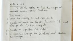
Lab 1, , Value of functions, Aim:, • To construct an applet to establish geometrically the correspondence of a number and its, image under a function., • To use this applet to find the images of numbers under various functions, • To use an applet to visualise the comparison of a function with an input-output machine., Concepts:, • Image of a number a under a function f is denoted by f (a), • Graph of a function is a collection of points (a, f (a)), Discussion :, For any number a,the ordered pair (a, f (a)) are the coordinates of a point on the graph of the, function f (x), so its y coordinate gives the value of f (a). We use this idea for constructing our, applet. Once such an applet is constructed, we can simply change the function and use it for, different functions., Sometimes we compare a function with a machine which gives an output, according to the definition, of the function, for a given input. In Activity 1.3 we use an Applet which helps us to visualise this, comparison. By this activity we get a clear idea about the domain of the function., , Activity 1.1 Functions, Procedure:, • Draw the graph of f (x) = x2 ., • Create a number slider a with increment 0.01, • Plot the points A(a, 0), B(a, f (a)), C(0, f (a))., (give inputs like A=(a,0))., • Draw the line segments AB and BC, using line segment tool., , To show the coordinates of a, point, right click on the point., Go to Object Properties → Basic → Show Label and select the, Name and Value option, , • Show the coordinates of A, B, and C., • Now drag the point A along the x axis (either click and drag the point or using slider - click, and drag the slider point to change the value ofa) and observe the movement of C on the y, axis., Using this, find the values of (2.3)2 ,(−1.8)2 ,(0.9)2 ,(2.9)2 . . ., 6

Page 9 :
1 Value of functions, , 7, , Save the file as Activity 1.1, , Activity 1.2 Values of Functions, Procedure:, , • Open the file Activity 1.1 and save as Activity 1.2, • Create an input box for f and change the function, using it., (Select input box tool, → Click on Graphics view, → give a suitable caption (say function), → linked object → f (x) = x2 → OK), • Similarly create an input box for the slider., , Change the functions accordingly and find the approximate values corrected to 3 decimal, places of the following, 1, , 33, , √, , 2, , 1.8, , 23, , p√, , 5, , (3.46), , −3, 2, , 1, , Function, , x3, , Input(x), Value(f (x)), , 3, , 1, Change the function to f (x) = , and observe how the point, x, C moves as the point A approaches the origin from either side., , We can set the number of decimal places, as follows;, Options → Rounding, → Select number of, decimal places., , Change the function to f (x) = [x] and observe the movement, of C according to A, , Activity 1.3 Function Machine, Procedure :, Use Applet ML 1.3, About the Applet, Three switches are provided on the machine, • GREEN :- Click to start the machine., • RED :- Click to stop the machine., • BLUE :- Click to reset., Using input boxes we can change the function and, the input number., The warning light provided on the machine turns, red if the input number is out of the domain of, the function., IT Maths Laboratory Manual

Page 10 :
1 Value of functions, , 8, , Change the function to f (x) =, √, √, i) 2, ii) 1.8, , √, , x and find the values of the following., q, iii) 23, , What happens if we give a negative number as the input ?, Change the function to f (x) =, i), , 2, 3, , ii), , −3, 7, , 1, x, , and find the values of the following., q, iii) 23, , What happens if the input is 0 ?, , Additional Activities, Activity 1.A Temperature Scales, Discussion, There are various scales to measure temperature. Perhaps the most popular ones are the Fahrenheit, and the Celsius scales., F (C) is the Fahrenheit temperature corresponding to the Celsius temperature C and they related, to each other as, 9, F (C) = C + 32, 5, • Plot the graph of the above function (Consider C as, the variable x), •, , From the graph identify the Celsius temperature at which the Fahrenheit temperature become, zero, , •, , From the graph identify the Fahrenheit temperature at which the Celsius temperature become, zero, , IT Maths Laboratory Manual, , While plotting the graph of, F (C) we have to use x instead of, C. So in order to get the graph, input 9x/5+32

Page 11 :
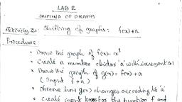
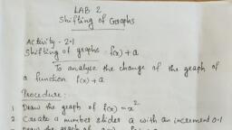
Lab 2, , Shifting of Graphs, Aim:, To analyse the changes in the graph of a function according to some slight changes in the definition, Concepts:, • Graph of a function, Discussion :, If we know the graph of the function f (x) we can obtain the graphs of the functions f (x) + a,, f (x + a), −f (x) and f (−x) by translation or reflection., This idea helps us to imagine the graphs of some functions if the graph of the base function is, known., This activity throws light on the concept of a family of curves., , Activity 2.1 Shifting of graphs : f (x) + a, Procedure:, , • Create a number slider a with increment 0.1, , Apply trace to the graph to, get a pattern.(rightclick → trace, on).To erase the pattern ,press, ctrl+F, , • Draw the graph of g(x) = f (x) + a, (Input:f+a), , Change the value of slider by, these methods :, , • Draw the graph of f (x) = x2, , •, , Observe how the graph of f (x) changes according to a, , • Create input boxes for editing function and slider a, Do the above observations for different functions such as |x|, [x], x3 etc, • Save this as Activity 2.1, , 9, , • Click on the slider point, and move, • Using Move tool, select, the slider and use arrow, keys, • Right click on the slider →, and turn on animation

Page 12 :
2 Shifting of Graphs, , 10, , Activity 2.2 Shifting of graphs : f (x + a), Procedure:, • Open a new GeoGebra window., • Draw the graph of f (x) = x2 ., • Create a number slider a with increment 0.1, • Draw the graph of g(x) = f (x + a). (Input:, f(x+a)), Observe how the graph of g(x), changes according to a., • Create input boxes for editing function and slider a., Generalise the above observations with different functions such as |x|, [x], x3 etc, • You may use the animation option to change the slider., • Save this as Activity 2.2, , Activity 2.3 Reflection of a Graph : −f (x), Procedure:, , • Open a new GeoGebra window., • Draw the graph of f (x) = x2, • Draw the graph of g(x) = −f (x) (Input: -f), Compare the graphs of f (x) and g(x)., • Create an input box for f and change the function to, i) x2 + 2, v) [x], , ii) x2 − 1, , iii)|x| − 1, , vi) x2 + 2x + 1, , iv) |x − 1|, , 1, vii), x, , Compare the graphs of f and g in each case. Write your findings., • Save this file as Activity 2.3, , IT Maths Laboratory Manual

Page 13 :
2 Shifting of Graphs, , 11, , Activity 2.4 Reflection of a Graph : f (−x), Procedure:, • Open new GeoGebra window, • Draw the graph of f (x) = x3, • Draw the graph of g(x) = f (−x) (Input: f(-x)), Compare the graph of f (x) and g(x), • Create an input box for f and change the function to, 1, i), ii) [x], iii) |x|, x, iv) x2, v) (x − 2)2, Compare the graphs of f and g in each case., Write your findings., • Save this file as Activity 2.4, , Additional Activities, Activity 2.A Translations of Graphs:1, Procedure:, , • Draw the graph of f (x) = x2 ., • Create a number slider a, with increment 0.1, • Draw the graph of g(x) = f (x − a) + a., Observe how the graph of g(x) changes according to a., • Create an input box for g and change the function to, i) f (x − a) − a, , ii) f (x − a) + 2a, , iii) f (x − a) + 3a, , iv) f (x − a) − 3a, , Observe the shift in the graph of g according, to the change in a., •, , Try to draw the pattern given in the figure., , IT Maths Laboratory Manual, , A function f (x) is an even function if f (−x) = f (x) and an odd, function if f (−x) = −f (x)., What is the speciality of the, graphs of odd and even functions?, Identify odd and even functions, discussed in this lab., Is there any function which is, neither odd nor even?

Page 14 :
2 Shifting of Graphs, , 12, , Activity 2.B Translations of Graphs: 2, • Draw the graph of f (x) = x2 ., • Create number sliders a and b , with increment 0.1, • Draw the graph of g(x) = f (x + a) + b., , • By adjusting the values of a and b transform the graph of x2 to that of the following functions., i), , (x + 2)2 − 3, , ii) x2 + 6x + 9, , iii) x2 − 4x + 6, , Activity 2.C Family of curves - using sequence command, Using sequence command, we can represent the family of curves obtained by shifting a graph, Procedure:, • Draw the graph of f (x) = x2, • In the input bar,, give the, Sequence[f+i,i,-3,3,0.2],, which, graphs of the functions, , command,, gives the, , In, the, input, command, Sequence[f+i,i,-3,3,0.2],, f is, function, i is variable, -3 is start, value, 3 is end value and 0.2 is, increment, , x2 − 3, x2 − 2.8, x2 − 2.6, . . . , x2 , . . . , x2 + 3, , Imagine the family of curves obtained by the following input commands and then draw them., 1. Sequence[f(x+i),i,-3,3,0.2], 2. Sequence[f(x-i)+i,i,-3,3,0.2], 3. Sequence[f(x-i)-i,i,-3,3,0.2], 4. Sequence[f(x-i)+2i,i,-3,3,0.2], , Create a slider a and input the Command Sequence[f(x-i)+a*i,i,-3,3,0.2], Create an input box for f and observe the pattern for different functions, , IT Maths Laboratory Manual

Page 15 :
Lab 4, , Trigonometric Functions, Aim:, • To create an applet to find the values of trigonometric functions and plot their graphs, • To establish some behaviours of trigonometric functions in different quadrants, Concepts:, • Concept of circular functions, • Graph of the function f is a collection of points of the form (a, f (a)) for all values of a in its, domain, Discussion :, If a point is rotated from (1, 0) along the unit circle centred at the origin, by an angle x radians,, the x and y coordinates of the point represent cos x and sin x respectively. We define all other, trigonometric functions in terms of cos x and sin x. We use this idea to construct our applet., , Activity 4.1 Values of Trigonometric Functions, Procedure:, Open a new GeoGebra window,do some initial settings as follows, Options→ Advanced → Angle unit → Radian, • Plot the point O(0, 0) (input O=(0,0)), • Draw a unit circle centred at the origin O, • Plot the point A(1, 0) (input A=(1,0)), • Create a number slider a with min value -10 , max, value 10 and increment 0.01. While creating the, slider, set its animation as increasing, • Plot another point A0 such that ∠ AOA0 = a radian, • Rename the point A0 as P (right click → Rename ), • Show the coordinates of P, • Join OP using a line segment, • Create an input box for the slider a., 18, , • To set the animation of a, slider as increasing, right, click on the slider and, in the object properties,, select increasing option, from the repeat dropdown, menu, • To create an angle AOA0, with measurement a, use, Angle with a given size, tool, click on A, O and, then give a as the angle in, the box

Page 16 :
4 Trigonometric Functions, , •, , 19, , Animate the slider,observe the coordinates of the point P, hence find the domain and, range of sin x and cos x, , •, , Find the values of sin x and cos x for the given values of x, x, , π, 3, , π, 4, , π, 6, , π, 2, , 0.3, , 0.6, , 2, , -1.5, , -3.1, , 7.5, , sin x, cos x, , For giving π in the input box, input:pi, , Identify the values of x for which sin x and cos x become 0,1,-1, • Save this file as Activity 4.1, , Activity 4.2 Graphs of Trigonometric Functions - 1, Procedure:, • Save file Activity 4.1 as Activity 4.2, using save as option, • Open Graphics 2 [view −→ Graphics, 2], • Plot the point B(a, y(P )). [y(P ) gives, the y coordinate of P], • Give trace to this point and animate, the slider, •, , Observe the path of this point., What does this path represent?, , • Save the file., , • We can see the path of the point using, locus tool also.To get the path,take the, locus tool, click on the point and on the, slider, • For analysing the graphs of trigonometric, functions, it is more convenient to mark, · · · −π2 , 0, π2 · · · on the x axis instead of ...1 ,0 ,1..., (For this right click on the Graphics 2., Go to Object Properties Change the x, Axis distance to π2 ), • We can draw the graphs of sin x and cos x, using input commands sin(x), cos(x) etc., , IT Maths Laboratory Manual

Page 17 :
4 Trigonometric Functions, , 20, , Activity 4.3 Graphs of Trigonometric Functions - 2, Procedure:, , • Open Activity 4.2 and save as Activity 4.3 using save as option, • Create an input box for the point B, • Change the definition of B as (a, x(P )), •, , Observe the path of this point, , •, , What does this path represent?, y(P ), 1, Redefine B as (a, y(P, ) ) and (a, x(P ) ), observe the path of P and identify the functions., , •, •, , What should be the definition of B for getting the graphs of sec x and cot x?, , •, , Observe the values of trigonometric functions, write their domain, range and complete, the following table.,
,
,
,
, π, 3π, Function, 0, π2, π, 3π, 2,π, 2, 2 , 2π, sin x, , Positive, Increasing, from 0 to 1, , cos x, , tan x, , Increasing, from 0 to ∞, , sec x, , cot x, , cosec x, , IT Maths Laboratory Manual

Page 18 :
4 Trigonometric Functions, , 21, , Additional Activities, Activity 4.A k sin(x), Discussion :, We construct an applet similar to that in Activity 4.1, using which we describe the functions, k sin(x), k cos(x) etc. for different values of k., Procedure :, Do the initial settings as in activity 4.1, • Create two sliders, k with Min = 0 and a with min value -10 , max value 10 and increment, 0.01.While creating the slider a, set its animation as increasing, • Draw a circle of radius k centered at the origin O(0,0), • Plot the point A(k, 0), • Plot another point A0 such that ∠ AOA0 = a radian, • Rename the point A0 as P, • Show the coordinates of P, • Join OP using a line segment, •, , What does the coordinates of the point P represent ?, , •, , Find the domain and range of k sin(x) and k cos(x) for different values of k, , • Open Graphics 2 and plot the graphs of k sin(x) and k cos(x) as we done in Activity 4.2., • Save this file as Activity 4.A, , Activity 4.B k sin(2x), Discussion :, We construct an applet using which we describe the functions k sin(2x), k cos(2x) etc., Procedure :, • Open Activity 4.A and save it as Activity 4.B, • edit the rotation of P as 2a ( Double click and edit ), •, , What does the coordinates of the point P represent ?, , • Open Graphics 2 and plot the graphs of k sin(2x) and k cos(2x), • Create an applet to describe k sin(ax) and k cos(ax), for different values of k and a, , IT Maths Laboratory Manual

Page 19 :
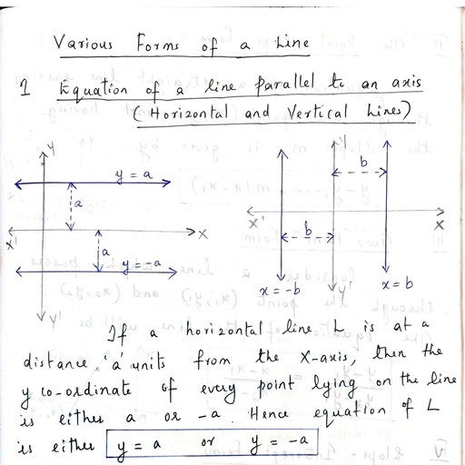
Lab 8, , Straight lines, Aim :, • To establish the role of coefficients and constant in the general equation of a straight line, • To explore geometrically the Normal form of a straight line, • To explore geometrically a family of straight lines, Concepts:, • General equation of a straight line, • Family of straight lines, • Normal form of a straight line, Discussion :, A straight line is represented as ax + by + c = 0 where a,b and c are constants. If c is changed,, while keeping a and b fixed, the straight line will change in a particular manner. Similar situations, are encountered with other constants. In this activity we explore the variations in the coefficients, and constant and its effect in the geometry of straight line., All the above mentioned activities will result in a set of straight lines having a common property., This set is called a family of straight lines., We also discuss the family of straight lines passing through a point of intersection of given lines., , Activity 8.1 General Form of Straight Lines, Procedure:, • Create three sliders a,b and c, • Draw the line ax + by + c = 0, • Change the values of a,b and c, •, , What happens to the line if, (i) a = 0, (ii) b = 0, (iv) a = b, , (iii) c = 0, , (v) a = -b, 36

Page 20 :
8 Straight Lines, , •, , 37, , Make the following changes and observe the corresponding changes in the line (Trace, option of the line may be used)., , 1. Change a alone, 2. Change b alone, 3. Change c alone, , Activity 8.2 Intersection of Two Lines, Procedure:, , • Draw two lines say, 3x − 2y + 4 = 0 and 2x + 5y − 6 = 0, • Create a slider k, • Input the equation 3x − 2y + 4 + k(2x + 5y − 6) = 0, , •, , It represents a line (why?), , •, , Change the value of k. Observe how the third line changes, , •, , For what value of k, the third line coincides with the first line?, , •, , For what value of k, the third line coincides with the second line?, , • Edit the equations of the first two lines so that they are parallel, , •, , What happens to the third line for different values of k, , Activity 8.3 Normal Form, Procedure:, • To find the normal form of a line geometrically, draw, the line and the perpendicular from the origin to the, line(use Perpendicular Line tool)., • Mark the point of intersection of the perpendicular, with the line., • Hide the perpendicular line and draw a line segment, from the origin to the line., IT Maths Laboratory Manual

Page 21 :
8 Straight Lines, , 38, , • Show the length of, the perpendicular, and the angle made, by it with the, positive direction of, the x axis., , Using Angle tool we can show the angle in the following ways, • Click on the positive direction of x axis and then on the, line segment.(Make sure that the line segment has been, drawn starting from the origin, otherwise we won’t get, the required angle.), , • Create an input box, for the line, , • Take a point - say C - on the positive direction of the x, axis. Using the tool click on C, the origin and the point, of intersection in that order. Hide C, , • save as Activity 8.3, , •, , Using this applet, write the normal form of the following lines, √, 1. x − 3y − 8 = 0, 2. x − y − 2 = 0, √, 3x − y + 8 = 0, , 3., , 4. 2x − 3y + 4 = 0, 5. x + y = 5, 6. 5x + 2y + 3 = 0, Write the equation of the lines in normal form for different values of ω and p (p is, the distance of the line from the origin and ω is the angle made by the normal with the positive, direction of x axis). Verify your answer using the above applet, Sl.No, , Value of ω, ◦, , Value of p, , 1, , 0, , 3, , 2, , 30◦, , 4, , 3, , 30◦, , 5, , 4, , ◦, , 2, , ◦, , 4, , Equation of the line, √, , 60, , 5, , 90, , 6, , 120◦, , 4, , 7, , ◦, , 4, , 150, , 3x y, + =4, 2, 2, , Activity 8.4 Shifting of Origin, Procedure:, • Using the applet, ML 8.4, About the applet:, ◦ You can click and drag at the, origin to shift the axes., ◦ You can change the curve and the, origin using corresponding input boxes, ◦ You can see the transformed, equation using check box, , IT Maths Laboratory Manual

Page 22 :
8 Straight Lines, , 39, , •, , Shift the origin, parallel to the x axis or y axis and observe the changes in the new, equation of the circle, , •, , What should be the new origin to get the transformed equation as x2 + y 2 = 4. Guess, the answer and check it., , •, , Find the transformed equation, if the origin is shifted to the point (1, 3). Check the, answer., , IT Maths Laboratory Manual

Page 23 :
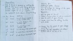
Lab 9, , Conic Sections, Aim :, • To show conics as the section of a cone as well as the locus of a point, Concepts:, • Cone and its section by a plane, • Locus of a point, Discussion :, Conic sections are curves obtained by the intersection a double cone by a plane. The angle at which, the plane cuts the cone determines the curve. The semi vertical angle of the cone, the position at, which the plane cuts the cone etc.. will determine the shape of the curve., We treat the curves as the locus of a point moving on a plane subjected to certain constraints., , Activity 9.1 Cutting of a Cone by a Plane, Using the applet ML 9.1, About the applet:, , In this applet we can see 3 open windows. Graphics 2 , 3D Graphics and the third one is View, of plane d, , 40

Page 24 :
9 Conic Sections, , 41, , Graphics 2, • There are three sliders and two check boxes here., • Using slider α you can change the semi vertical angle of the cone., • Using slider β you can tilt the plane, • Using slider “Position of the plane” you can change the position of the plane., • Using the check boxes we can show or hide the cone and the plane., 3D graphics, You can see the 3D view here, using Rotate 3D graphics view tool, you can rotate the entire, view to see it from a convenient angle., View of plane d, You can see the curve, obtained by intersecting the cone with the plane., Procedure:, Change the value of β for a fixed α. Observe the curves for different values of β., α, , Curve, , 25◦, , 30◦, , 45◦, , 50◦, , Circle, Parabola, Ellipse, Hyperbola, Circle, Parabola, Ellipse, Hyperbola, Circle, Parabola, Ellipse, Hyperbola, Circle, Parabola, Ellipse, Hyperbola, , β, 90◦, 25◦, 25◦ < β < 90◦, , For what values of β do we get the curves - circle, ellipse, parabola and hyperbola?, Change the position of the plane and observe the corresponding change in the shape of the, curve, Change α and observe corresponding change in the curve., , IT Maths Laboratory Manual

Page 25 :
9 Conic Sections, , 42, , Activity 9.2 Locus of a point moving equidistant from given points, Procedure:, • Plot two points A and B and join them (Using, line segment tool), • Create a number slider a with min=0 and max=10, • Draw circles of radius a centred at A and B, • Plot the points of intersection of the circles and give, their trace., • Give animation to the slider a, •, , Observe the path of the moving point. Describe the path., , • Save this file as Activity 9.2, , Adjust the increment of the slider as 0.01 or less to get a continuous, path. If we use Shift key together with the arrow keys to move the, slider, it will decrease the speed of the slider by one tenth. If we use, Ctrl key, speed will be increased 10 times, , Activity 9.3 Locus of a point the sum of whose distances from two given points is a, constant, Procedure:, • As in Activity 9.2, create a slider a, • Plot two points A and B and join them., • Draw a circle of radius a centred at A and another, circle of radius 10 − a centred at B, , We can create this applet by, editing the radius of the circle, centred at B of the previous Activity 9.2, , • Plot the points of intersection of the circles and give, their trace., • Give animation to the slider a, • Observe the path of the moving points. Identify the, curve traced., (We can show the path of the moving point using, Locus tool. For this, take the Locus tool, click on, one of the points of intersection and on the slider., Similarly click on the other point of intersection and, on the slider ), , •, , Change the distance between A and B and observe the change in the shape of the, curve, , •, , What happens to the curve when B approaches nearer and nearer to A?, IT Maths Laboratory Manual

Page 26 :
9 Conic Sections, , •, , 43, , What is the maximum possible distance between A and B to get a path?, , Activity 9.4 Locus of a point the difference of whose distances from two given points, is a constant, Procedure:, • As in Activity 9.2, Create a slider a, • Plot two points A and B, • Draw a circle of radius a centred at A and another, circle of radius a + 4 centred at B, • Plot the points of intersection of the circles and give, their trace., • Give animation to the slider a, • Draw another set of circles of radius a centred at B, and of radius a + 4 centred at A, • Plot the points of intersection of these circles and give their trace., • Give animation to the slider a, •, , Observe the path of the moving points.Identify the curve traced., (Here also we can use the Locus tool as in Activity 9.3), , Activity 9.5 Locus of point equidistant from a point and a fixed line, Procedure:, • Draw a line and plot a point C outside the line., • Draw perpendicular to the line through C., • Plot the point of intersection D of the line and its, perpendicular., • Create a slider a with min = 0, max = 15 and increment 0.01, • Draw a circle of radius a centred at D and plot its, point of intersection E with the perpendicular line., • Draw a line through E and parallel to the first line., • Draw a circle of radius a centred at C and plot its points of intersection with the last line, drawn. Trace on these points., • Give animation to the slider a, •, , Observe the path of the moving points. Identify the curve traced., , • Draw the path using Locus tool, •, , Change the distance between the point and the first line and observe the change in, the shape of the curve, , IT Maths Laboratory Manual

Page 27 :
9 Conic Sections, , 44, , Additional Activities, Activity 9.A Focus - Diretrix Definition, Discussion :, We discuss Parabola, Ellipse and Hyperbola as the locus of a point moving on a plane, keeping a, specific ratio of distance from a fixed line and a fixed point. Procedure :, • Create two sliders a, with min = 0 , max = 10 and, increment 0.01 and b with min = 0 , max = 5 and, increment 0.01, • Draw the line x = 0 and plot a point A on the positive, side of the x axis., • Draw the lines x = a and x = −a, • Draw a circle of radius ab centred at A., • Plot the point of intersection of the circle with the, lines x = a and x = −a ( If necessary, you can change, the values of the sliders, so that the circle meets the, lines.), • Trace the points of intersection, • Hide the axes, Set b=1 and animate slider a, •, , Observe the path of the points. Can you identify the curve ?, , • Using Locus tool, draw the path of the points., •, , Change the value of b and observe the path. Can you identify the curves for different, values of b ?, , •, , Try to define a parabola,an ellipse and a hyperbola in terms of distances from a fixed, line and a fixed point., , Activity 9.B Apollonius Circles, Discussion :, We discuss the locus of a point moving on a plane, keeping a specific ratio of distance from two, fixed points., Procedure :, • Create two sliders a and r with Min = 0 and increment 0.01. Create an input box for a., • Plot two points A and B and join them, • Draw a circle of radius r centered at A and another circle of radius ar centered at B, • Plot the point of intersections of the circles and trace them. Find the locus of the points, using Locus tool., •, , Observe the path for different values of a, IT Maths Laboratory Manual

Page 28 :
9 Conic Sections, , •, , 45, , Can you connect this with internal and external division of a line ?, , IT Maths Laboratory Manual

Page 29 :
Lab 13, , Limits, Aim :, • To geometrically explore the concept of the limit of a function at a point., Concepts:, • Value of a function at a point, • Graph of a function, Discussion:, We geometrically explore the concept of limit at a point. We discuss the existence and different, cases of non existence of limit, the nature of the graph at a point where limit exists/does not exist,, the concept of left limit and right limit etc.., We geometrically interpret some standard limits also., , Activity 13.1 Geometrical Interpretation of Limits, Procedure:, Use the applet 13.1-Limits, About the applet :, , • You can see the graph of a function f (x), 3 points A, B, P on, the x axis, corresponding points, A1 , B1 , P1 on the graph and A2 ,, B2 , P2 on the y axis, • ’NAME’ Check Box: By clicking on it you can show/hide the, names of the points, • VALUE Check Box: By clicking on it you can show/hide the x coordinates of the points A,, B and P and the y coordinates of the points A2 , B2 and P2, • Slider h: Using this we can bring the points A and B towards P, • Input box a: To change the position of P, 59

Page 30 :
13 Limits, , 60, , • Input box f : To change the function, Initial settings, • f (x) = x2, • a=2, • h=1, • Show the names of the points, , Gradually change the value of h from 1 to 0. Observe the movements of the points.What happens to A2 and, B2 as A and B approaches P ?, Show the values of the points. Set h=1 and gradually bring it to 0. Observe the values.What happens to the, x coordinates of the points A and B? What happens to the, y coordinates of A2 and B2 ?, , We can record the value of, points to spreadsheet as follows. Open spreadsheet view, −→ Spreadsheet., Right click on A1 −→ record, to spreadsheet −→ tick Row, limit(10) −→ Close. Similarly, record the point B1 to spreadsheet., , We can observe that as the x coordinates of A and B approach to 2, the y coordinates of A2 and, B2 approach 4., If we call the x coordinates of A and B as x, then the y coordinates of A2 and B2 are f (x), So we observe that as x → 2, f (x) → 4, ie, the limit of f (x) at x = 2 is 4, What happens to the points A, B, A2 and B2 when h = 0, , Activity 13.2 Limit of Rational Functions, Procedure:, , • In the above applet, change the function to f (x) =, , x2 − 4, x−2, , • Move the slider h from 1 to 0, •, , What is the limit of this function at x = 2, , •, , What happens to the points A2 and B2 when h = 0 (Refer Activity 3.2 ), , IT Maths Laboratory Manual

Page 31 :
13 Limits, , 61, , Activity 13.3 Limit of Piecewise Functions, Procedure:, Using the above applet, discuss the limit of the following functions, (, x2, if x ≤ 2, at x = 2, 1. f (x) =, 2x + 1 if x > 2, (Input If[x<=2,x^2,2x+1]), What happens to f (x) as x approaches to 2 from left and right?, (, x2, if x ≤ 2, and discuss the limit at, 2. Change f (x) =, 2x, if x > 2, x=2, Discuss the existence of limit for the following functions, 1, ,, at x = 0, x, (, 1, if x ≤ 0, 2. f (x) =, 2, if x > 0, , , if x < 0, x − 2, 3. f (x) = 0, if x = 0, , , x+2, if x > 0, (, x2 − 1, if x ≤ 1, 4. f (x) =, 2, −x − 1, if x > 1, 1. f (x) =, , (Input If[x<0,x-2,x>0,x+2,0], Or, If[x<0,x-2,x==0,0,x+2]), , Activity 13.4 Limit of Trigonometric Functions, Procedure:, •, , •, , Plot the graphs of sin x and x in the same, graphics view. Zoom it at the origin. What do you, see? What inference do you get from this?, , Using the applet used in the previous activity,, sin x, discuss the limit of, at x = 0, x, , Plot the graphs of x2 , sin(x2 ),, sin2 x, tan(x2 ) and tan2 x on, the same graphics view, Zoom, it at the origin and what do you, see? What inference you get, from this?, , Activity 13.5 Limit of Exponential and Logarithmic Functions, Procedure:, • Input a=0.We get a slider in the Algebra view. Show it in the graphics view by clicking on, it, • Draw the graph of the function f (x) = ex − a, • Input y = x to get the line, • Using Reflect about line tool, click on the graph and on the line, we get the reflection of, the graph of ex on the line y = x, which represents the graph of loge (x), IT Maths Laboratory Manual

Page 32 :
13 Limits, , 62, , • Using the slider a, move the graph of f downwards until the line becomes tangent to the, curve, •, , What happens to the reflection ?, , •, , What are the definitions of the functions represented by the curves?, , • Zoom it at the origin until the three curves seem to be one, •, , What do you infer from this?, , •, , Write down some limits using this inference, , Additional Activities, Activity 13.A Some more problems, Procedure:, , 1., 2., , 3., , 4., , With the help of the applet, discuss the limit of the following functions,
, f (x) = sin x1 at x = 0,
, f (x) = x sin x1 at x = 0,
, Draw the lines y = x and y = −x. Why does the graph of x sin x1 lie between these lines?,
, f (x) = x2 sin x1 at x = 0,
, Draw the curves y = x2 and y = −x2 . Discuss the existence of the limit of x2 sin x1 at 0, with the help of these graphs,
, √, f (x) = x sin x1 at x = 0, Draw the parabola y 2 = x. Discuss the existence of limit of the above function with the help, of this curve, , IT Maths Laboratory Manual

Page 33 :
FT, , Lab 18, , Functions, , A, , Aim:, • To visualise one to one and onto function geometrically, , • To restrict the domain and codomain of functions so as to make it a bijection, , R, , • To visualise composition of two functions geometrically, Concepts:, , D, , • One to one and onto functions, • Composition of functions, , Discussion :, We discuss the properties of graphs of One to One and onto functions.Discuss about how to, determine whether a given function is one to one and onto geometrically,how to restrict the domain, and codomain of functions so as to make them bijections.We plot the graph of g ◦f from the graphs, of the functions f and g, , T, , Activity 18.1 One to One and Onto Functions, Procedure, , R, , • Draw the graph of f (x) = x2, , • Create a slider a and plot the point (0, a), , E, , • Draw a line through the point and perpendicular to the, y axis., , SC, , If for any value of a, the line meets the graph of, a function at more than one point, can we say whether, the function one to one or not. Why ?, , If for all values of a, the line meets the graph of a function at at least one point,, can we say whether the function onto or not. Why ?, Using above applet, say whether the function f : R → R defined above is one to one, or onto., 4

Page 34 :
18 Types of functions, , 5, , • Keeping above ideas in mind, one can say whether a function is one to one or onto, by, observing its graph, even without drawing the horizontal line., • Save the file as Activity 18.1, , FT, , Activity 18.2 One to One and Onto function 2, Open Activity 18.1 and save as Activity 18.2, Create Input box for f, , Draw the graphs of the following functions defined from R to R and say whether they, are one to one or onto. Find the range of the function in each case., i, ii, iii, , One-One, , Onto, , Range, , A, , Function, x2 + 2, x3 − 3x2 + 3, 3 sin(x), , D, , x−2, i) f : R − {3} → R − {1} defined by f (x) =, x−3, , , 1, x, ii) f : [−1, 1] → −1,, defined by f (x) =, 3, x+2, x, iii) f : R → R defined by f (x) =, 1 + |x|, , R, , The following functions are defined from a subset of the set of real numbers. Say whether, they are one to one or onto. Find their range., , What is the peculiarity of the range of an onto function ?, , T, , Activity 18.3 Bijective Functions, We can make a function one to one by restricting its domain and onto by restricting its co-domain., If we define a function to its range, it becomes onto. From the graph of a function we can easily, select a suitable subset of the domain to make it one to one, , •, , R, , Procedure, , Consider the function f : R → R defined by, f (x) = x2 + 1. Is it one-one or onto ?, , E, , • Draw the graph of above function, , SC, , Redefine the function by restricting its codomain so that it becomes onto, • From the graph of the function we can see that if we, restrict the domain to [0, ∞) the function becomes, one to one., , • So the function f : [0, ∞) → [1, ∞) defined by f (x) =, x2 + 1 is a bijection., • Draw the graph of above function. (Use input command if(x>=0,x^2+1) or if(x>=0,f) or, Function(f,0,infinity), IT Maths Laboratory Manual

Page 35 :
18 Types of functions, , 6, , • If we define f : (−∞, 0] → [1, ∞) then also it becomes a bijection. Draw the graph of this, function., Restrict domain and co-domain of the following functions so that they becomes, bijections, Function, |x − 2|, x2 − 3x + 3, | sin x|, , Domain, [2, ∞), , Co-domain, , FT, , i, ii, iii, , For each of above functions find one more domain which make them one to one. Draw, the corresponding graphs., , A, , Activity 18.4 Composition of functions, , We create an applet to describe the composition of two functions geometrically, , • Draw the graph of f (x) = x2 and g(x) = sin x, • Draw the line y = x, • Create a slider a, , D, , • Plot the point A(a, f (a)), , R, , Procedure, , • Draw the line passing through A and parallel to x axis, and plot its point of intersection B with the line y = x, • Draw the line passing through B and parallel to the y, axis and plot its point of intersection C with the graph, of the function g, , T, , • Draw the following lines and take their point of intersection D, – Passing through A and parallel to the y axis, , R, , – Passing through C and parallel to the x axis, , • Complete the rectangle ABCD and hide the lines, , E, , Write the co ordinates of the points B,C and D in terms of a, , SC, , Trace the point D and animate the slider.What does the graph represents?Use locus, tool to get the clear path., , • Create input boxes for the functions f and g., Following functions are of the form (f ◦ g)(x). Identify f and g and use above applet, to trace the path of the given functions, i)sin |x|, , ii) elogx, IT Maths Laboratory Manual

Page 36 :
18 Types of functions, , 7, , Additional Activities, Activity 18.A Composition - Physical situation, , FT, , We discuss a physical situation in which the concept of composition of functions included., Use Applet ML18.A, , D, , R, , A, , About the applet, , A rope is wound on a disc of radius 1 meter . A red ball is attached at the end of the rope., A green ball is attached to a point on the circumference of the disc by means of a rod which, always remains horizontal. A yellow ball is attached to the green ball using two pulleys. We can, wind/unwind the rope using the slider a. When a=0 all the balls lie on the base line, the horizontal, line passing through the centre of the disc., , T, , If we unwind the disc so that the red ball moves x meters down wards, let the green ball moves, y meters and yellow ball moves z meters from the base line. We take the movement of a balls as, positive, if it is above the base line and negative if it is below the base line., , R, , Write y as a function of x., Write z as a function of y., , E, , Write z as a function of x., Suppose we pull down the red ball at the rate of 2m/s. Write x, y and z as functions of, the time t., , SC, , Suppose that the red ball freely falls under gravitational force. Write x, y and z as functions, of the time t., , Activity 18.B One-one and onto property of functions, We have seen how to check the one to one and onto properties of functions.Now let us check these, properties of composition of such functions.Consider the following functions in an applet, IT Maths Laboratory Manual

Page 37 :
18 Types of functions, f, , oneone, , onto, , 8, g, , oneone, , g◦f, , onto, , oneone, , x−4, 2x + 3, x−4, 3, , x2, 1, x, 1, ,x > 0, x, , x2, , x3, , x2, , |x|, , x − [x], , 3x − 1, , x2, , sin x, , x2, , cos x, , x3, , FT, , x2 + 1, , x − [x], , R, , A, , x2, , and verify the properties, , D, , • f is one to one and g is one to one implies g ◦ f is one to one, • f is onto and g is onto implies g ◦ f is onto, , • g ◦ f is one to one implies f is one to one and g need not be one to one, , SC, , E, , R, , T, , • g ◦ f is onto implies g is onto and f need not be onto, , IT Maths Laboratory Manual, , 0nto

Page 38 :
FT, , Lab 19, , Invertible Functions, , A, , Aim:, • To explore invertible functions, , R, , Concepts:, • Bijective functions, • Inverse of a function, , D, , • Composition of functions, Discussion :, For a given real number a,we discuss the method of finding the value of f −1 (a),from the graph of, f (x).Methods of drawing graph of inverse of a function is also discussed., , Activity 19.1 Inverse of a Function 1, , T, , If f is an invertible function and (x, y) is a point on the graph of f then f (x) = y and f −1 (y) = x., We use this idea to find the value of f −1 (a), for given values of a, from the graph of f (x)., Procedure :, • Draw the graph of f (x) = x2 , x ≥ 0, , R, , • Create a slider a, • Plot the point A(0, a), , • Draw the line passing through A and parallel to the x axis, , E, , • Plot the point of intersection B of the above line with the curve, • Draw the line through B, perpendicular to the x axis, , SC, , • Plot the point of intersection C of the above perpendicular line, with the x axis, • Hide the lines and draw the line segments AB and BC, , • Show the coordinates of C, Using this applet, how can we find an approximate value of, , a?, , Find approximate values of the following, 9, , √, , a for a given value of

Page 39 :
19 Types of functions, i), , √, , 3, , 10, ii), , √, , 4.5, , • Note : If we need more accuracy we can increase the number of decimal places. (Options →, Rounding), • Save the applet as Activity 19.1, , FT, , Activity 19.2 Inverse of a Function 2, Procedure :, Use the applet ML19.2, About the applet:, , This applet is similar to that we created in the above activity.In addition there are two input boxes, to edit the function f and the slider a, , Function, i, , √, 3, , ii, , log2 10, , iii, , 1, √, 5, , A, , Select suitable functions and find approximate values of the following, Value, , Activity 19.3 Inverse of a Function 3, Procedure, , D, , R, , 4, , • Find the inverse of the function f (x) = x3, , • Draw the line y = x, , T, , • Draw the graphs of f (x) and f −1 (x), , R, , Compare the graphs of f and f −1 with respect to the above line. What do you, observe ?, If we know the graph of function f how can we draw a rough sketch of the graph of, f −1 ?, , E, , • Using the tool Reflect about line we can draw the reflection of a graph of a function about a, line (Click on the graph of the function and then on the line), , SC, , • Draw the graph of function f (x) = x2 and find its reflection on the line y = x, represent the graph of a function? Why?., , Does it, , • To get the graph of inverse of a function ,restrict the domain of the function -if needed-in, order to make it one to one.Draw the graph of the function in the restricted domain and find, its reflection on the line y = x, Find the inverse of the following functions algebraically and draw its graph. Draw, the graph of the given function and find its reflection on the line y = x. Verify whether it, coincides with the graph of the inverse of the function. Find the domain and range of the, given function., IT Maths Laboratory Manual

Page 40 :
19 Types of functions, Function, i, , √, , 11, Inverse, , Domain, , Range, , x+2, , x2 − 4x + 7, , iii, , x, x+2, , FT, , ii, , • In algebra view ,the equation of a reflected curve is shown only in its parametric form., • The command Invert(f) gives the graph of inverse of a function and its equation in, explicit form.It is not necessary to restrict the domain to get the inverse.But this, command also has some drawbacks, , A, , • It works only if the function contains just one x.If f is a quadratic function ,then the, command :Invert(CompleteSquare(f)) gives the inverse, • If f is a rational function with first degree polynomial in numerator ,then the command, Invert(PartialFractions(f)) gives the inverse, , R, , • In CAS view ’invert’ command directly works even if the function contains more than, one x, , D, , Activity 19.4 Composition and Inverse, Procedure :, , • * Use the applet Activity 18.4, • Give f (x) = 3x − 2 and g(x) =, , x+2, 3, , T, , Observe the graphs of f ◦ g and g ◦ f . What do you see ? Why it happens so ?, • Find the inverse of the following functions and verify your answer using the above applet., , R, , [* Or we can verify the answer by directly inputting g ◦ f and f ◦ g in the input bar,without, using the Applet ], f −1 (x), , f (x), x−2, 3, , ii, , (3 − x3 ) 3, , E, , i, , SC, , 1, , Additional Activities, , Activity 19.A Self Invertible Functions, 1, We know that the inverse of f (x) =, is the function itself. We may call it as a self invertible, x, function. Here we discuss a method to generate self invertible functions from existing one. The, IT Maths Laboratory Manual

Page 41 :
19 Types of functions, , 12, , logic behind the construction is that the graphs of self invertible functions are symmetric with, respect to the line y = x ( why ?), Procedure, 1, and the line y = x, x, , FT, , • draw the graph of the function f (x) =, , • The graph is symmetric with respect to the line. If we shift it along the line, it keeps its, symmetry, • Create a slider a, , • Create the function g(x) = f (x − a) + a. Find the simplified form of g using the command, Simplify(g)., , A, , • Create an input box for f and save the applet as Activity 19.A, , We get different self invertible functions for different values of a. Find some functions, and verify it using the applet Activity 18.4, 2 −3 2x − 5, ,, ,, generate more self invertible functions., x 2x 2x − 2, , Activity 19.B Composition Machine, , R, , Starting from the functions, , D, , Last year we have studied functions as input -output machines,which gives outputs corresponding, to the given inputs.Here we compare composition of functions with combination of machines in, which output of one of the machine is the input of the other., , E, , R, , T, , Use Applet ML19.A, About the applet;, , SC, , In 3D graphics we can see two machines combined together.Output of the first machine is the input, of the second.There are three buttons on the machine, Blue,Green ,and Red,in order to refresh,start, or stop the machine.Two indicator lights are provided which turns red if the corresponding input, is not suitable for the machines.From the Graphics view we can edit the functions as well as the, input number, Procedure, , • Set f (x) = 2x and g(x) = x2, Find the values of (g ◦ f )(2) and (g ◦ f )(3) andg ◦ f (−3), IT Maths Laboratory Manual

Page 42 :
19 Types of functions, , 13, , • Set f (x) = 2x and g(x) =, , √, , x, , Find the values of (g ◦ f )(2) and (g ◦ f )(3), , FT, , What happens to the indicators if we give -3 as the input? why?, , What can you say about the domain of the function g in order to define g ◦ f ?, √, • Set f (x) = x and g(x) = x2, , A, , Find the values of (g ◦ f )(2) and (g ◦ f )(1) andg ◦ f (0), , What happens to the indicators if we give -2 as the input? why?, , R, , Find the domain in which (g ◦ f )(x) = x, , SC, , E, , R, , T, , D, , Find the domain in which (f ◦ g)(x) = x., , IT Maths Laboratory Manual

Page 43 :
FT, , Lab 20, , Inverse Trigonometric Functions 1, , A, , Aim:, , • To make trigonometric functions invertible by restricting the domain and codomain with the, help of their graphs, , R, , • To draw the graphs of inverse trigonometric functions, • To find the value of inverse trigonometric functions from graphs of corresponding trigonometric function and from unit circle, , • Trigonometric functions, • Inverse trigonometric functions, , D, , Concepts:, , Discussion :, We discuss how to restrict domain and codomain of a trigonometric function so as to make it, invertible, , T, , Activity 20.1 Making Invertible, , As we have seen in Activity 18.3 we can make a function One-One and Onto by restricting its, domain and range. In this activity we discuss trigonometric functions and make them bijections., , R, , Procedure :, , E, , • Mark the distance on x axis in terms of π2 . (Right click on Graphics View → Graphics → x, π, axis → Distance → Select, from the drop down menu), 2, • Draw the graph of f (x) = sin x., , SC, , π, • By observing the graph we can see that if we re define f as f : [ −π, 2 , 2 ] → [−1, 1] it becomes, a bijection., , • Draw the graph of the above function ( use the command If(-pi/2<=x<=pi/2,f).), , 14

Page 44 :
20 Inverse Trigonometric Functions 1, , By selecting suitable domain and range, make all trigonometric functions invertible., Draw the corresponding graphs and complete the following table (There are infinitely many, possible domains which makes a trigonometric function bijective.You may select any one, among them), , Function, sin x, cos x, tan x, cosec x, sec x, cot x, , Domain, π, [ −π, 2 , 2], , Range, [−1, 1], , FT, , •, , 15, , A, , • Save the GeoGebra file as Activity 20.1, , Activity 20.2 Graph of Inverse Trigonometric Functions, , • Open the GeoGebra file Activity 20.1, , D, , • Mark the distance on x axis as ...-1,0,1,2,3,..., π, and that on y axis in terms of, 2, • Draw the line y = x, , R, , We know that the graph of f −1 is obtained by reflecting the graph of f on the line y = x. We use, this idea to draw the graph of inverse trigonometric functions., , • Open the graphs of trigonometric functions, (bijective) one by one and reflect them on the, line y = x (using Reflect about Line tool.), , •, , T, , • save the file as Activity 20.2, , Write the domain and range of the of the inverse trigonometric functions., , Damain, , Range, , E, , R, , Function, sin−1 x, cos−1 x, tan−1 x, cosec−1 x, sec−1 x, cot−1 x, , SC, , We can draw the graphs of inverse trigonometric functions using input commands, , Function, sin−1 x, cos−1 x, tan−1 x, cosec−1 x, sec−1 x, cot−1 x, , Command, sin^-1(x), cos^-1(x), tan^-1(x), cosec^-1(x), sec^-1(x), cot^-1(x), , or, or, or, or, or, or, , asin(x), acos(x), atan(x), asin(1/x), acos(1/x), pi/2-atan(x), , IT Maths Laboratory Manual

Page 45 :
20 Inverse Trigonometric Functions 1, , 16, , Activity 20.3 Value of Inverse Trigonometric Functions from Graph, In Activity 19.1 we discussed the method of finding f −1 (a),from the graph of the function f , for, given values of a. We use this method to find the values of inverse trigonometric functions from, the graphs of the corresponding trigonometric functions., Use the applet ML20.3, , FT, , About the applet:, In this applet graph of a function f is given .Using an input box we can edit the function.Using, another input box we can change the value of, the slider a.The point A on the y-axis represents, (0, a). x co ordinate of the point C represents, f −1 (a), , sin, , A, , Find the values of sin−1 (0.5) and, −1, , (− √12 ), , √, , 3, 2 ), , tan−1 (5), , cos−1 (0.5), , cosec−1 (−2), , sec−1 ( √23 ), , cot−1 (−4), , D, , sin−1 (, , R, , Find the values of the following. If possible write in terms of π otherwise write in decimal, form (may be an approximate value ), , Activity 20.4 Value of Inverse Trigonometric Functions from Unit Circle, We have defined sin x and cos x with the help of a unit circle centered at the origin. Here we use, the reverse of that process to find the values of sin−1 x and cos−1 x for given values of x., Use applet MLActivity 20.4, , T, , About the applet, , R, , • For a given value of a we can find the values of sin−1 a, cos−1 a or tan−1 a. We can select, the required one using the check boxes., • We can change the value of a using the slider, , Procedure :, , E, , • If we select the check box ’sine’ we get a semi circle of radius 1 on the positive side of the x, axis and a point B, with y co-ordinate a, moves along y axis according to a., , SC, , • Suppose we are asked to find sin 0.85 (refer the figure given below ), we rotate the point, P from A(1, 0) by an arc of length 0.85 (or by an angle of 0.85 radian ) in anticlockwise, direction. The y coordinate of P gives sin 0.85 that is 0.75, , • If we are asked to find sin−1 0.75, then the question is reversed, that is, what should be the, angle (or arc length ) of rotation of P in order to get its y coordinate as 0.75 ?. So we plot, the point B(0, 0.75), the corresponding point on the circle and find the arc length (or angle)., So from the figure sin−1 0.75 =).85 (It may be an approximate value ). If the rotation of P, is in the clockwise direction we take the value as negative., IT Maths Laboratory Manual

Page 46 :
17, , FT, , 20 Inverse Trigonometric Functions 1, , A, , • In a similar manner we can find cos−1 a for give values of a, , The figure given above shows that tan−1 2 = 1.11. Discuss the reason, , •, , Discuss a method to find tan−1 a, using the applet, for given values of a, , •, , Using the applet find the following values, sin−1 (−0.6), , cos−1 (0.8), , cos−1 (−0.5), , SC, , E, , R, , T, , sin−1 (0.4), , D, , R, , •, , IT Maths Laboratory Manual, , tan−1 (5), , tan−1 (−3)

Page 47 :
Application of integrals, , A, , Aim, , FT, , Lab 31, , • To find the area enclosed by curves using definite integrals, , R, , Concepts, • Definite integrals, , Activity 31.1 Area bounded by x axis, , D, , Discussion, We discuss different methods of finding area enclosed by curves with the help of GeoGebra, , If the curve y = f (x) in [a, b] is above the x axis then the area of the region bounded by the, curve, x axis x = a and x = b is given by, Z b, A=, f (x)dx. We can find this using the Input Command Integral(f,a,b), , T, , a, , Procedure, • Create two number sliders a and b and Input boxes for them, , R, , • Draw the graph of the function f (x) = x2 ., , E, , • Find the area enclosed by the curve y =, f (x), x axis, x = 0 and x = 2. [For this set, a = 0, b = 2 and give the Input Command, Integral(f,a,b)], Find the area enclosed by the curve, y = x2 , x axis, between, , SC, , 1) x = −1 and x = 3, 2) x = −5 and x = 0, , • Create a Input Box for the function f (x)., Find the area enclosed by the curve y = x2 − 1, x axis between x = −1 and x = 1., Find the required area and complete the following table., 62

Page 48 :
31 Application of integrals, , 63, , Enclosed Region, y 2 = x, x axis, x = 1, x = 4, y2, x2, 16 + 9 = 1, x2 + y 2 = 4, y = sin x, x axis, x = π, x = 2π, , Area, , FT, , Sl.No., 1, 2, 3, 4, , Hint: For question number 2 and 3 draw the whole region using input bar, • save as Activity33.1, , Activity 31.2 Area of a region which is above and below x axis, , A, , If a curve lies on both sides of the x axis it is not possible to find its area by direct integration., We discuss different methods of solving such problems., Procedure, , • Find the area enclosed by the curve y = x2 − 3, x axis x = −3 and x = 3, , Z, , R, , • Open the applet Activity33.1. Set f (x) = x2 − 3, a = −3 and b = 3., 3, , x2 − 3 dx ?. Give the reason., , What is the value of, , D, , −3, , What is the area of the portion below the x axis?, [To find this find the points of intersection A and B of, the curve with the x axis and give the input command, Integral(f,x(A),x(B)], , T, , What is the area of the portion above the x axis?, Find the total area of the region., Alternate Method, , R, , • Edit the function as f (x) = |x2 − 3|. Set a = −3 and, b=3, Find the area using the input command Integral(f,a,b), , E, , Find the required area and complete the following table., , SC, , Sl.No., 1, 2, 3, 4, , Enclosed Region, y, y, y, y, , Area, , = sin x, x axis, x = 0, x = 2π, = x3 , x axis, x = −2, x = 4, = |x| − 2, x axis, x = −1, x = 3, = 3x + 2, x axis, x = −1, x = 1, , √, If the area bounded by the curve y = 3x and the line x = 12 is divided in the ratio 1:7, by the line x = a, then find the value of a. (If necessary change the maximum value of the slider, b), IT Maths Laboratory Manual

Page 49 :
31 Application of integrals, , 64, , Activity 31.3 Combination of curves, We discuss the methods of finding the area bounded by a combination of curves., , FT, , Find the area of the region bounded by the curve x2 + y 2 = 32 and the line y = x in the, first quadrant., Procedure, • Draw the circle x2 + y 2 = 32 and the line y = x., • Identify the enclosed region., , • Find the area under the line y = x using the input, command a=Integral(x,0,x(A))., , R, , • Find the area under the circle using the input command b=Integral(sqrt(32-x^2),x(A),x(B))., , A, , • Mark the point of intersection A of the line with the, circle. Also mark the point of intersection B of the, circle with the x axis., , Find the required area., (, x, • Define the function as f (x) = √, , if 0 < x < x(A), if x(A) < x < x(B), , D, , Alternate method, 32 − x2, , For this give the input command f(x)=If(0<x<x(A),x,x(A)<x<x(B),sqrt(32-x^2), Find the area using the input command Integral(f,0,x(B)), Find the area of the following regions., , T, , 1) Region in the first quadrant bounded by x axis, the line y =, , √, , 3x and the circle x2 +y 2 = 4, , 2) Region lying above x axis and included between the circle x2 + y 2 = 8x and inside of the, parabola y 2 = 4x., , R, , 3) Region enclosed between the two circles x2 + y 2 = 4 and (x − 2)2 + y 2 = 4., 4) The Region {(x, y) : 0 ≤ y ≤ x2 , 0 ≤ y ≤ x + 1, 0 ≤ x ≤ 2, , E, , Activity 31.A Availability of medicine in the blood, , SC, , Medicine can be administered to patients in different ways. For a given method let c(t) be the, concentration of the medicine in the blood t hours after the dose is given.Over the time interval, 0 ≤ t ≤ a the area between the grapf of c(t) in the interval [0, a] indicates the availability of the, medicine for the patients body over the time., Since GeoGebra does not have the time axis, we will change the independent variable to x., Two methods Method 1 and Method II for administrating the medicine is governed by the, functions f (x) and g(x) represented as follows, f (x) = 5(e−0.2x − e−x ), f (x) = 4(e−0.2x − e−3x ), , In this activity we try to explore the availability of medicine to the patients body, IT Maths Laboratory Manual

Page 50 :
31 Application of integrals, , 65, , Procedure, • Create a slider a with minimum value 0 and maximum value 24 , corresponding to 24 hour, period, • Create the function f (x), , FT, , • Create the function g(x), • Evaluate the integral of f from 0 to a using integral function .This can be achieved by inputting, Integral(f, 0, a), • Evaluate the integral of g from 0 to a as above .In the algebra view we can see that two, variables are created for the area of the two figures, • Move the slider a and observe the change in the areas, , A, , If 4 is the value of a , which area is more?Which method provides better availability of the, medicine?, , R, , If 24 is the value of a, which area is more? Which method provides better availability of, the medicine?, , SC, , E, , R, , T, , D, , Move the slider in such a way that the areas of both the functions are same.What does, this condition signify in medical perspective?, , IT Maths Laboratory Manual

Page 51 :
FT, , Lab 34, , Vectors, , A, , Aim, • To explore the concept of vectors and vector operations, , • To explore the concepts of direction angles and direction cosines, , R, , • To resolve a vector in given directions, , • vectors and vector operations, , D, , Concepts, , • Direction angles and direction cosines of a vector, • Components of a vector, , T, , Discussion, We familiarise some tools and commands for the construction of vectors and vector operations in, GeoGebra, using which we discuss some problems on vectors which helps to get the geometry of, vectors.Discuss direction angles and direction cosines of vectors geometrically.We also discuss the, method of resolving a vector in given directions ., , R, , Tools and Commands, Let’s familiarise some tools and commands used for the construction of vectors and vector, operations in GeoGebra., • Vector tool or the Input Command Vector(Point,Point) gives the vector which starts, from the first point and ends at the second point., , E, , • The Input Command Vector(Point) gives the vector starts from the origin and ends at the, point., • Vector from Point tool, by clicking on a point and on a vector gives the vector starts from, the point and parallel to the given vector., , SC, , • The Input Command Point(Point,Vector) Gives the end point of the given vector which, starts from the given point., • Translate by Vector tool, by clicking on an object translates it by the magnitude of the, vector in its direction., • |u| gives the modulus of ~u, • If a is a scalar and u is a vector, then the Input command au or a*u gives the vector a~u, , • If u and v are vectors, the Input command u+v gives ~u + ~v and u-v gives ~u − ~v ., 75

Page 52 :
34 Vectors, , 76, , Activity 34.1 Construction of Vectors, , Do the following problems, , 2. Construct the vector 3î + ĵ + 2k̂ starting from the point, (2, −2, 3)., 3. Construct the vector joining the points (1, −2, 4) and, (3, 2, −2)., 4. Construct three mutually perpendicular vectors with, same initial point (2, 2, 2)., , A, , 5. Construct the parallelogram whose adjacent sides are, represented by the vectors ~a = 2î + 2ĵ + 3k̂ and ~b =, î − 4ĵ − 3k̂, , FT, , 1. Construct the vector 3î + ĵ + 2k̂., , 6. Create a slider a and a vector ~u. Construct the vector a~u. Observe the vector by changing, the value of a., , R, , 7. Construct the vector ~u = 4î − 3ĵ + 3k̂. Construct the unit vector in the direction of ~u. Also, Construct the vector having magnitude 5 in the direction of ~u., , D, , Activity 34.2 Direction ratios and Direction Cosines, Procedure, , • Plot the points O(0, 0, 0), A(1, 0, 0), B(0, 1, 0), C(0, 0, 1) and P (4, 3, 2)., −−→, • Construct the vector OP ., , T, , −−→, • Find the angles α, β and γ made by OP with the positive direction of x axis, y axis and z, axis. [input : α=Angle(A,P), β=Angle(B,P),γ=Angle(C,P)]. Hide the points A, B and C., , R, , • Draw the perpendicular from P to the x axis and plot, its point of intersection D with x axis., Write the x coordinate of D., , E, , Find cos α without using the input command, cos(α). Similarly find cos β and cos γ., , SC, , If ~r = xî + y ĵ + z k̂ write l = cos α, m =, cos β, n = cos γ in terms of x, y, z., Prove that cos2 α + cos2 β + cos2 γ = 1, , Open Graphics View and create an input box for the point P (It is not possible to create input box, in 3D Graphics), Edit the co ordinates of the point P such that it lies on the x- axis .What happens to the, direction cosines?What happens if P lies on the y-axis or z-axis?, IT Maths Laboratory Manual

Page 53 :
34 Vectors, , 77, , Edit the co ordinates of P such that it lies on the xy plane . What happens to n?Write l, and m in terms of α only., , Activity 34.3 Components of a vector, , FT, , Procedure, , Construct the components vectors of the vector ~r = 2î + 5ĵ − 3k̂ along the positive direction of the, coordinate axes., , • Plot the point A(2, 5, −3) and construct the vector ~r using the input command r=Vector(A)., , • Construct the component vectors., , R, , A, , • Plot the points B(x(A), 0, 0), C(0, y(A), 0) and D(0, 0, z(A). Draw the segments AB, AC and, AD., , D, , Create an input box for the point A. Write the vector ~r and its component vectors, for the following positions of A, (3, 2, 0), (0, 5, −2), (0, 4, 0), (0, 0, −3), , Express the vector ~r = 4î + 4ĵ as the sum of two vectors which are parallel to ~u = 3î + ĵ and, ~v = î + 6ĵ, • Construct ~r as in the last discussion, • Construct the vectors ~u and ~v ., , T, , • Draw the lines passing through the origin and parallel to the vectors ~u and ~v . For this give the input, commands Line((0,0,0),u) and Line((0,0,0),v), , R, , • Draw the line passing through the point A (end point, of ~r) and parallel to ~v . Plot its point of intersection, B with the line parallel to ~u, −−→, −−→, • Draw the vectors OB and BA where O is the origin., , E, , Note: Since all the vectors in the above discussion are in the xy-plane this construction can be, done in the graphics view also., , SC, , Additional Activities, , Activity 34.A Components of a vector in space, Express the vector ~r = 2î + 5ĵ + 3k̂ as the sum of the vectors parallel to ~a = 4î + 2ĵ, ~b = −î + 4ĵ, and ~c = î + ĵ + 5k̂, IT Maths Laboratory Manual

Page 54 :
34 Vectors, , 78, , • Construct, the, points, P (2, 5, 3), A(4, 2, 0), B(−1, 4, 0), and, C(1, 1, 5) hence construct the vectors, ~r, ~a, ~b and ~c., , FT, , • Draw the line passing through P and parallel to ~c and plot its point of intersection D, with the xy plane. (xy plane is available in, the 3D view by default. Otherwise give the, input command z=0.), • Draw the line passing through O and parallel to ~a, , A, , • Draw the line passing through D and parallel to ~b and plot its point of intersection, E with the line constructed in the last step., −−→ −−→, −−→, • Draw the vectors OE, ED and DP ., , Activity 34.B The Vector Clock, , R, , Can you express the vector ~r = 2î + 5ĵ + 3k̂ as the sum of the vectors parallel to ~a = 4î + 2ĵ,, ~b = −î + 4ĵ and ~c = î + ĵ ? Why ?, , D, , In this activity a clock is viewed from the perspective of vectors. The origin is assumed as the, center of the clock and vectors are drawn from the origin to each hour position., , Procedure:, • Create a point A(0,0), • Create a point B(0,5), , T, , • Using the Sequence command, create a list of points which are a result of rotation of B by an, angle 300 , 600 , 900 , . . . 3300 . This can be achieved by the command Sequence(Rotate(B, −k ∗, (360/12)0 ), k, 0, 11). A list l1 is created., , R, , • Draw vectors from A to the list created in the previous step by using Sequence command., This can be achieved by Sequence(V ector(A, l1(k), k, 1, 12). A list of vectors l2 is created., • Translate the vector l2(2) to the tip of l2(1 using the command T ranslate(l2(2), l2(1)). A, point C is created., , E, , • Draw a vector from the tip of l2(1) to the point C by using the command V ector(l2(1), C), • Translate the vector l2(3) to the tip of C using the command T ranslate(l2(3), C). A point, D is created., , SC, , • Draw a vector from the tip of C to the point D by using the command V ector(C, D), • Translate the vector l2(4) to the tip of D using the command T ranslate(l2(4), D). A point, E is created., , • Draw a vector from the tip of D to the point D by using the command V ector(D, E), • Continue this for all the vectors which represent the hands of the clock., What is the sum of the vectors of the hands of the clock?, IT Maths Laboratory Manual

Page 55 :
34 Vectors, , 79, , The sum of the vectors can be achieved using a single command Sum. In the input bar, type Sum(l2). This will create a vector whose sum is the vector sum of all the vectors in, the list l2., , FT, , What is the sum of all the vectors if the vector corresponding to 2:00 is dropped off?, Use the command Sum by including all the items in the list l2 except the one corresponding, to 2:00. This can be achieved by the command, Sum(l2(1) + l2(2) + l2(4) + l2(5) + l2(6) + l2(7) + l2(8) + l2(9) + l2(10) + l2(11) + l2(12)), , What if the 1:00 hour handle is dropped?, , A, , Can you generalise this activity?, , R, , If two consecutive vectors are removed, say the vector corresponding to 1:00 and 2:00, are removed, what will happen to the resultant?, If the vectors corresponding to 1:00 and 3:00 are removed, what is the resultant?, , SC, , E, , R, , T, , D, , If all the twelve vectors start from (0,-5) corresponding to 6:00, what will the resultant, be? To do this in the algebra view right click on the point A and in the object properties, change the coordinates from (0,0) to (0,-5), , IT Maths Laboratory Manual

Page 56 :
FT, , Lab 37, , The Plane, , A, , Aim, , R, , • To derive the equation of a plane, , • To explore the geometry of planes satisfying different conditions, , D, , Concepts, , • Concept of plane, , T, , • Concept of vector and vector operations, , R, , Discussion, We derive the equation of a plane passing through a given point and perpendicular to a given, vector. We also discuss some problems on planes and construct them, , Activity 37.1, , Procedure, , E, , We derive the equation of plane passing through a given point and perpendicular to a given, direction., , SC, , • Plot the point A(3, 2, 2) and construct the vector ~a = 2î + ĵ + 5k̂., , • Construct the plane passing through A and perpendicular to ~a., , −−→, • Take any point B on the plane and draw the vector ~u = AB., Find ~a · ~u at different position of B. Why it happens so?, 87

Page 57 :
37 3D 8, , 88, , Detach the point B from the plane (either use Attach / Detach Point tool or edit, any one of the coordinates of B). Observe the, change in ~a · ~u. What happens to it when B is, not on the plane? Why?, , FT, , Write a necessary and sufficient condition for a point to be on the plane. Write the, algebraic form of this condition. Hence find, the equation of the plane., , A, , Derive the equation of the plane passing, through the point (x1 , y1 , z1 ) and perpendicular to the vector aî + bĵ + ck̂., , Activity 37.2 Tools and Commands, , R, , We discuss some tools and Input Commands for constructing planes, Commands, , Output Plane, , 1, , Plane(Point,Plane), , Passes through the given point and parallel to the given plane, , 2, , Plane(Point,Line), , 3, , Plane(Line,Line), , 4, , Plane(Point,Point,Point), , Contains the given points, , 5, , Plane(Point,Vector,Vector), , Contains the given point and parallel to the vectors, , 6, , Plane(Polygon), , Contains the polygon, , 7, 8, 9, , Plane(Conic), Perpendicular plane(point,line), Perpendicular plane(point,vector), , Contains the given conic, Contains the point and perpendicular to the line, Contains the point and perpendicular to the vector, , D, , Input Command, , Passes through the given point and contains the line, , Contains the lines (if they are intersecting), , T, , Sl.No, , Tools, Sl.No, , Name of Tool, , R, , Direct input of the equation gives the corresponding plane, , Output Plane, , Plane through 3 Points, , 2, , Plane, , 3, , Perpendicular Plane, , Same effect of commands 8 and 9, , 4, , Parallel Plane, , Same effect of Command 1, , Same effect of Command 4, , Same effect of Commands 2, 3, 4 and 6, , SC, , E, , 1, , Construct the planes as per the conditions given in the following problems. You can use, any tool to construct vectors and lines but use only the Perpendicular Plane tool to construct, the plane. Note the method of construction in your observation book. You can verify the result, using any direct tool., 1. Plane passes through the point (2, 2, 3) and parallel to the vectors 3î − 2ĵ + k̂ and î + 3ĵ., 2. Plane passes through the point (1, −2, 3), (1, 1, 4) and (−3, 2, 2), IT Maths Laboratory Manual