Page 2 :
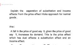
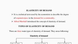
ORDINAL UTILITY APPROACH (INDIFFERENCE CURVES ANALYSIS) 99, , (if) Tastes and preferences or the indifference, map of the consumer is given., , (iii) Prices of the two commodities remain, unchanged., , (iv) There is a rise (or fall) in consumer’s income., , Given these assumptions, the effect of a change, , (rise) in the income of the consumer can be explained, through Fig. 6.25., , Y-Commodity, , , , , , 9° QQQ 8B B, B xX, X-Commoadity, , Fig, 6.25, , In Fig. 6.25, the X-commodity is measured along, the horizontal scale and Y-commodity is measured, along the vertical scale., , Given prices of two commodities and money, income of the consumer, the price line AB can be, drawn. As income of the consumer increases, prices, of X and Y remaining the same, price line shifts to, right to A,B, and A>B>. If the indifference map of, the consumer is super-imposed upon price lines, the, price lines AB, A,B, and A,By are tangent to IC,,, IC, and IC; at R, S and T respectively. By joining, these points with the origin, it is possible to draw, the income-consumption curve ICC which slopes, upwards from left to right. The ICC tells what, quantities of the two commodities the consumer, buys, if prices of two commodities remain constant, but the income of the consumer changes (rises). At, these equilibrium positions, the consumer buys OQ,, OQ, and OQ, of X-commodity and OP, OP, and OP,, of Y-commodity respectively. Thus, the increase in, the money income of the consumer leads to a rise in, the quantities bought of both the commodities. The, Income effect in this case is positive because both, the commodities are normal or superior., , The income effect is negative when one of the, two commodities is inferior. In case of an inferior, commodity, the quantity bought of the commodity, falls with an increase in the money income of the, consumer. The purchase of superior or normal, commodity, however, increases with an increase in, money income., , If X-commodity is inferior, given Y-commodity, as normal, the income effect can be explained through, Fig. 6.26., , Icc, , , , Y-Commodity, , , , , , , , , , , , , , o Q3Q,Q Bo 8B ax, X-Commodity, , Fig. 6.26, , In Fig. 6.26, it is assumed that commodity X is, inferior, while the commodity Y is norm: Originally, given the prices of two commodities and income of, the consumer, the price line is AB. If the-money, income increases, prices of the two commodities, remaining the same, the price line shifts to A,B, and, A,B). As the map of indifference curves is superimposed upon them, the equilibrium of the consumer, shifts from the original position R to $ and T. If, these points are joined with the origin, it is possible, to draw the income-consumption curve ICC which, initially slopes upwards from left to right and, subsequently bends backwards towards the vertical, scale. At the original equilibrium position R, the, consumer buys OQ of X and OP of Y. As income, increases, the consumer raises the purchase of, normal commodity Y to OP, at S and OP) at T. In, case of the inferior commodity X, the quantity bought, is reduced from OQ to OQ, and OQ, at points S and

Page 3 :
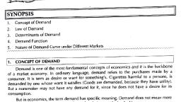
100, , T respectively. Thus, with an increase in income,, the quantity bought of normal commodity Y, increases, whereas the quantity bought of inferior, commodity X gets reduced., , If Y-commodity is inferior and X-commodity is, , normal, the income effect can be explained through, Fig. 6.27., , Y-Commodity, >, , xa, , , , , , , , , , , , , , , , oO QQ; B QB, B, X, X-Commodity, , Fig. 6.27, , In Fig. 6.27, the original price line is AB. Given, prices of two commodities, as income of the, consumer increases the price line shifts to AB, and, AB . When the indifference map of the consumer, is super-imposed upon these price lines, the price, line AB, A,B, and A,B, are tangent to IC), IC, and, IC, at R, S and T respectively These are the positions, of equilibrium. By joining these points with origin,, it is possible to draw the income-consumption curve, ICC which initially slopes upwards and later bends, downwards towards the horizontal scale. This shape, of the ICC implies that commodity X is normal but, the commodity Y is inferior. At R, S and T, consumer, buys OQ, OQ, and OQ, quantities of X-commodity, and OP, OP, and OP, quantities of Y-commodity, respectively. So as income of the consumer increases,, the purchase of normal commodity X is increased, and that of inferior commodity Y is reduced., , The shape of the income-consumption curve, (ICC) can indicate the nature of the commodities., , This is shown through Fig. 6.28., , MICRO-ECONOMIC THEORY, , Y-Commodity, , , , ° X-Commodity, , Fig, 6.28, , Ifthe income-consumption curve is of the shape, ICC,, both X and Y-commodities are normal and, superior. If the income-consumption curve is of the, shape ICC, commodity X is inferior and the, commodity Y is normal or superior. If the incomeconsumption curve is of the shape ICC;, the, commodity X is normal or superior whereas the, commodity Y is inferior., , It was discussed above that incomeconsumption curve ICC is positively sloping, when, the commodities are normal. The normal goods may, either be luxuries or necessaries. If the quantity, bought of a commodity increases more than, proportionate to an increase in income, the, commodity can be considered luxury but if the, quantity bought of a commodity increases less than, proportionate to an increase in income, the, commodity can be considered necessary. On the, basis of the shape of the income-consumption curve,, it is possible to distinguish whether a commodity is, a luxury or a necessary commodity through Fig. 6.29., , Y, ICC,, , x Icc,, , no, , Q, , €, , §, , or ICC,, Ss, , o X-Commodity x, , Fig. 6.29

Page 5 :
104, , expenditure curve (E,E,) in case of inferior commodity, slopes negatively. These three cases are shown in, Fig, 6.35,, , 6.12 PRICE EFFECT, , The equilibrium of the consumer can be affected, not only by a change in money income of the, consumier but also by a change in price of one of, the two commodities. If the income of the consumer, and price of one of the two commodities remains, constant but the price of the other commodity, changes, the resultant change in the quantities, bought of the commodities or shift in the equilibrium, of the consumer can be termed as the price effect., , The price effect can be analysed on the basis, of the assumptions given below :, , (i) The tastes or preferences of the consumer, remain unchanged., , (ij) Income of the consumer remains the same., , (ii) Price of one of the two commodities remains, constant., (iv) Price of the other commodity falls (or rises)., , Suppose consumer has to buy two commodities, X and Y. Price of Y and the money income of the, consumer remain constant but the price of X, commodity falls. The price effect in such conditions, can be explained through Fig. 6.36., , , , , , , , , , , , , , , , , , , , yi, , = iA, , DZD, , °, , z, , 9 P, , SEP;, , Z T, ie PCS, , ICg, oO Gee memos By X, X-Commodity, , Fig. 6.36, , In Fig, 6.36, X-commodity is measured along the, horizontal seale and Y-commodity is measured along, the vertical scale. Given the prices of two commodities, and money income of the consumer, originally AB is, the price or budget line. If money income of the, consumer and price of Y remain the same but the, price of X falls, the price line shifts to AB, and AB)., If consumer’s indifference map is super-imposed, upon these price lines, the equilibrium of the, , MICRO-ECONOMIC THEORY, , consumer gets determined at R, S and T. By joining, these points, it is possible to draw the price., consumption curve (PCC) which slopes downwards, from left to right. The PCC indicates the different, quantities of the two commodities that the consumer, would buy if the income and price of Y are constant, but the price of X falls. In Fig. 6.36, consumer buys, OQ of X and OP of ¥ at R, OQ; of X and OP; of Y at, § and OQ, of X and OP, of Y at T. It is clear that, consumer goes on increasing the purchase of X as, the price of this commodity falls. On the opposite, if, the price of X rises, other things remaining the same,, it is also possible to show that the quantity bought, of X-commodity can decline., , In case the price of X-commodity remains, unchanged but the price of Y falls, the price effect, can be shown through Fig. 6.37., , Ay, , a, , Y-Commodity, DER>, , , , , , QQQ B x, X-Commodity, , Fig. 6.37, , In Fig. 6.37, as the price of Y falls, money income, and price of X remaining the same, the price lines, are AB, A,B and A,B. If the indifference map is, placed upon them, equilibrium gets determined at R,, Ss and T respectively. By joining these points the, price-consumption curve (PCC) is drawn which slopes, positively. The consumer buys OQ of X and OP of, Y at R, OQ; of X and OP, of Y at S and OQ, of X, and OP, of Y at T. Thus, consumer increases the, purchase of Y-commodity as its price falls. On the, contrary, if the price of Y rises, other things remaining, the same, it is possible to show that the quantity, purchased of Y commodity falls., , : If the price of X falls, the PCC can assume, different shapes, In Fig. 6.36, it is shown that the, PCC slopes downwards from left to right. In addition,, itmay be stated that PCC may be a horizontal straight