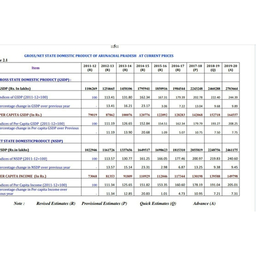
Page 1 :
The cardinal utility approach was based upon, awed assumptions like rationality of, nit possibility of measurement of utility,, , Maal measurement of utility, constancy of the, , oe utility of money and single commodity, , urchase. All these assumptions in general -and, cardinal measurement of utility in particular gave, , rise to serious objections. In view of the, shortcomings of the traditional theory of consumer, behaviour, an alternative theory for explaining, consumers’ behaviour was developed. This, alternative theory was called as ordinal utility, , approach or the indifference curves theory., , The indifference curves theory was originally, conceived by the writers like Pareto, Edgeworth and, Fisher. In 1915, E.E.-Slutsky made a highly significant, contribution through his essay, ‘On the Theory of, the Budget of the Consumer’. This essay served to, consolidate the ordinal utility hypothesis and the, demand analysis based upon it. In 1928, a paper, entitled, ‘A Reconstruction of the Theory of Value’, was published by J.R. Hicks and R.GD. Allen., These writers not only made a scathing attack upon, the cardinal utility analysis but established the, indifference curve approach on the basis of the, notion of ordinal utility. The landmark development, In this connection took place in 1939, when J.R. Hicks, m his famous work, Value.and Capital, provided a, pias and sophisticated framework of ordinal utility, , a each to explain consumers’ behaviour ina more, , sie and scientific manner. In the present chapter,, , vill peti of the indifference curves theory, © discussed., , certain, , Bie io ler A, , xa oto, , > sop

Page 2 :
82, , 6.2 ASSUMPTIONS OF INDIFFERENCE, CURVES OR ORDINAL UTILITY, ANALYSIS, , Z _Hicks-Allen ordinal utility approach or the, indifference curves analysis rests upon the following, main assumptions :, , () Assumption of rationality : \n this analysis,, the supposition is taken that the consumer is rational., He attempts to secure maximum satisfaction through, his expenditure on combinations of two or more, goods. In this connection, it is also assumed that, consumer has complete information of the availability, of goods, satisfaction therefrom and the prevailing, prices of products in the market., , (ii) Assumption of ordinal measurement of, utility : The indifference curves analysis dismissed, the notion of cardinal measurement of utility. Since, utility is subjective and psychological and problems, exist in the exact and quantitative measurement of, utility and, therefore, the addition or subtraction of, utility is impossible. The indifference curves theory, recognises that there can still be the possibility of, ordinal measurement of utility. The concept of ordinal, measurement of utility means the comparisons of, satisfaction can be made by the consumer. Although, it is difficult for a consumer to tell how much more, or less satisfaction he can get from one or the other, commodity, yet it is realistic for him to indicate which, combination of goods can give more or less, satisfaction. It means consumer can rank or arrange, the different combinations in accordance with higher, or lower level of satisfaction that they can provide., , (iif) Assumption of scale of preferences : As, the ordinal utility approach recognises the ability of, consumer to make comparisons of satisfaction, it, gives way to the preference hypothesis. On the basis, of more or less satisfaction expected from the different, combinations, the consumer can prepare in mind a, “list of priorities’ or a ‘scale of preferences’. He can, indicate specifically his preferences about the various, combinations of goods. In this connection, two, things should be remembered. Firstly, the choice or, preference of the consumer is independent of how, much more or less satisfaction one combination gives, compared with the other combination. The choice is, determined simply on the basis of the fact that one, combination can give more satisfaction than the other., Secondly, consumers’ preferences about combinations, of goods are not influenced by market prices of, , MICRO-ECONomic THEORY, , goods. Satisfaction alone is the sole cri, preparing the mental scale of preferences,, , (iv) Assumption of weak ordering ; Th, indifference curves theory is based on the wea, ordering of preferences. The weak order implies Bs, apart from preferring one combination to another,, the possibility also exists that the consumer may be, indifferent about certain combinations of goods, If, there are two combinations A and B, weak ordering, of preferences implies that consumer may prefer 4, to B or B to A or he may be indifferent about these, two combinations. In contrast, strong ordering of, preferences means consumer is very specific about, his preferences. If A is preferred to B, he will always, choose A rather than B when these two combinations, appear before him and there is no possibility either, of reversal of order of preferences or any indifference, between the combinations. The indifference curves, theory assumes weak ordering form of preference, hypothesis and recognises the possibility of, indifference on the part of consumer between various, combinations of goods., , (¥) Assumption of transitivity : The assumption, of transitivity means that there is no contradiction, in the preferences of a consumer. Suppose consumer, prefers combination A to combination B, and then, combination B to combination C, transitivity means, he must prefer A also to C. Similarly, if the consumer, indicates that he is indifferent between combination, A and B, then he is also indifferent between B and, C, the transitivity will imply that consumer must also, be indifferent between A and C. So transitivity, signifies that tastes and preferences of the consumer, are consistent. If A is preferred to B, B is preferred, to C but A is not preferred to C, it will suggest nontransitivity or lack of consistency in the tastes and, preferences of the consumer., , (vi) Assumption of continuity : The Hicks-Allen, ordinal utility approach takes also the assumption, of continuity. It means the consumer is capable of, visualising even very very minor differences in, satisfaction in various combinations of goods and, can accordingly rank all the conceivable combinations, of goods. It is on the basis of the assumption of, continuity that the indifference curves theory could, denote a series of combinations of two goods about, which consumer is indifferent through a smooth and, continuous curve., , (vii) Assumption of consistency ; The, , indifference curves theory rests upon the assumption, that the behaviour of the consumer is consistent., , terion fo,

Page 3 :
oR, 5 1pp08e consumer prefers combination A to B, and, ae C, then his behaviour is consistent if he prefers, a C. Similarly if he is indifferent between A and, : and B and C, the consistency requires that he, “ould also be indifferent between A and C. If in, , n, he prefers A to C or vice-versa, his, , an situation i ., pehaviour will be regarded as inconsistent., , (viii) Assumption of non-satiation : This, assumption of indifference curves theory means that, a consumer prefers more quantity of any commodity, to the lesser quantity of it. For instance, combination, \ includes 2 oranges + 3 bananas and combination, p includes 3 oranges + 3 bananas, then the, combination B is better than A. It includes more, quantity of oranges, the quantity of bananas, remaining the same. Consequently, the consumer will, prefer combination B to the combination A., , 6.3 MEANING OF INDIFFERENCE CURVE, AND INDIFFERENCE MAP, , Indifference curve, , When a consumer has to buy combinations of, {wo or more commodities, some of those combinations, yield greater satisfaction while the other combinations, yield lesser satisfaction. The consumer, accordingly, prepares a list of priorities or scale of preferences, in his mind. A combination that yields maximum, satisfaction is assigned the highest rank or the highest, order, Those combinations which yield lesser and, lesser satisfaction are accorded lower ranks or, priorities. Suppose there are two commodities,, bananas and oranges and consumer feels that the, combination of 30 bananas and 12 oranges can yield, the maximum satisfaction, he will buy this combination, first of all, If the combination of 25 bananas and 11, oranges, 20 bananas and 10 oranges, 15 bananas, and 9 oranges and 10 bananas and 8 oranges yield, lesser and lesser satisfaction, the consumer will place, them in his scale of preferences while purchasing, them in the same descending order., , In the scale of preferences of the consumer, there, can be certain combinations of the two commodities, which are supposed to yield exactly the same, satisfaction. In case of such combinations, the, consumer cannot accord any higher or lower priority, while making the purchase. He will be neutral or, 'ndifferent about those combinations., , : Such combinations of oranges and bananas, wie: which the consumer is indifferent or which, Yield equal satisfaction to the consumer are shown, , pINAL UTILITY APPROACH (INDIFFERENCE CURVES ANALYSIS), , 83, , through the hypothetic illustration given in Table 6.1, TABLE 6.1—Indifference Schedule, , , , , , Combination Oranges Bananas, A 1 20, B 2 14, Cc 3 9, D 4 5, E 5 2, , , , , , , , , , , , The combinations A, B, C, D and E shown in, Table 6.1 are supposed to be such combinations of, oranges and bananas as yield exactly equal, satisfaction. Between combinations A (1 orange +, 20 bananas) and B (2 oranges + 14 bananas),, consumer increases the quantity of orange by 1 unit., At the same time, he reduces the purchase of bananas, by 6 units. The gain in satisfaction due to larger, purchase of oranges can be fully offset by the loss, in satisfaction due to a smaller purchase of bananas., This is known as compensating variation in, satisfaction. Similar compensating variation can take, place between combinations B and C, between C, and D, and between D and E. As all these, combinations yield exactly the same satisfaction, one, combination can not be preferred to the other. The, consumer may buy any one of them. It means the, consumer will be indifferent about all these, combinations., , If all those combinations which yield equal, satisfaction to the consumer are represented through, a curve, such a curve is called as an indifference, curve. The indifference curve is defined by Baumol, as “the locus of points each of which represents a, collection of combinations of goods that will be, equally satisfactory to the individual concerned.”, In the words of Hicks, “It is the locus of the points, representing pairs of quantities between which the, individual is indifferent so it is termed as an, indifference curve.”, , Since the indifference curve shows such, combinations of two commodities which yield equal, satisfaction to the consumer, it is also called as an, Iso-utility curve. The term ‘iso’ means equal. So a, curve showing combinations yielding equal utility, or satisfaction is termed as the iso-utility curve or, indifference curve., , On the basis of combinations of oranges and, bananas given in Table 6.1, it is possible to draw, the indifference curve of the consumer. It is shown

Page 4 :
84, through Fig. 6.1., , , , Fig. 6.1, , In Fig. 6.1, oranges are measured along the, horizontal scale and bananas are measured along, the vertical scale. The points A (1 orange + 20, bananas), B (2 oranges + 14 bananas), C (3 oranges, +9 bananas), D (4 oranges + 5 bananas), E (5 oranges, + 2 bananas) represent those combinations of two, commodities which yield equal satisfaction to the, consumer and he is indifferent about them. By joining, the points A, B, C, D.and E, the indifference curve, is drawn. The indifference curve IC slopes, downwards from left to right and it is convex to the, , origin., , Indifference Map, The different combinations of two commodities, that lie upon the same indifference curve provide, equal satisfaction to the consumer and he is neutral, or indifferent about them. Suppose consumer wants, to have a combination of two commodities that can, give more satisfaction than all-those combinations,, it is clear that this combination yielding higher, satisfaction cannot lie upon:the same indifference, curve. It will lie at some higher indifference curve., Similarly, if a combination of these two commodities, can provide lesser satisfaction than the combinations, lying upon the given indifference curve, even this, combination cannot lie upon the same indifference, curve. It will lie upon some lower indifference curve., In this way, there can be a number of indifference, curves, each representing a different level of, Satisfaction, The indifference curves at higher levels, indicate such combinations of commodities that can, aineet stistcion. On the oppo, the, at lower levels indicate such, , MICRO-ECONOMIC. THEORY, , combinations of commodities that can yield lease, satisfaction. Thus there can be a collection of, indifference curves corresponding to varying level, of satisfaction. This collection of indifference curve,, is an indifference map., , ’ So indifference map-can be defined as a.seriey, of indifference curves representing different eye),, of satisfaction. Higher the indifference curve, highe,, is the level of satisfaction. Lower the indifference, curve, lower is the level of satisfaction, ‘The, indifference map can be shown through Fig. 6.2, , Y, , , , ° Q Q)0,Q, x, Oranges, , Fig. 6.2, , In Fig. 6.2, there is a series of indifference curves, ICj, IC, IC; and'IC,. It signifies an indifference map,, A straight line OR is passed through these, indifference curves. Combinations A, B, C and D lie, respectively on IC,, IC>, [C3 and IC4. Combination A, includes OQ of oranges + OP of bananas., Combination B is comprised of OQ, of oranges +, OP; of bananas. Since combination B includes more, quantities of both oranges and bananas than the, combination A, therefore, B gives more satisfaction, than A. Similarly combination C includes OQ, of, oranges + OP, of bananas. In this combination, there, are more quantities of both the commodities than in, combination B. So C.can give more satisfaction than, B. In the same way, combination D includes OQ; of, oranges + OP; of bananas. As there are more, quantities of both the commodities in combination, D than in the combination C, the former can give, more Satisfaction than the latter. It is thus clear thal, a combination lying upona higher indifference curve, can give more satisfaction than a combination lying, upon a lower indifference curve,

Page 5 :
Dopp, i tM ARGINAL RATE OF SUBSTITUTION, 6:, , if thiere are such combinations of two, moditieS, oranges and bananas, that give equal, comm ction to the consumer, it means an increase, gatisia yantity of oranges must be accompanied, reduction in the quantity of bananas. The, lity of equal satisfaction from alternative, ations can exist, if the gain in satisfaction, que 10 increased quantity of oranges is offset by, ihe loss if satisfaction due to a smaller purchase of, bananas The rate at which the marginal or last, is substituted in place of some, , unit of orange 3 z, juamity of bananas, 1S termed as the marginal rate, , 7 substitution of oranges for bananas., , The concept of marginal rate of substitution of, X commodity (say, oranges) for Y commodity (say,, bananas) Was defined by J.R. Hicks as “the quantity, of Y which would just compensate the consumer for, the loss of marginal unit of X.” According to Leftwitch,, “The marginal rate of substitution of X for Y, MRSxy) is defined as the amount of Y, the consumer, , ( : es 7, is just willing to give up to get an additional unit of, , x”, The concept of marginal rate of substitution can, be explained with the help of Table 6.2., , with @, possibl, combin, , TABLE 6.2—Marginal Rate of Substitution, , , , , , [Combinations Oranges | Bananas MRS of, , | (X) (Y) Oranges, , | for Bananas, | (MRS), [aa 1 20 =, , B 2 14 6:1, , | tae 3 9 Sel, , | D 4 4:1, , | E 5 2 Sick, , , , , , , , , , , , Combination A (1 orange + 20 bananas) gives, as much satisfaction as the combination B (2 oranges, * 14 bananas). It means the consumer gives up 6, bananas and in place of it gets 1 more orange. In, other words, consumer: substitutes one orange in, ie of 6 bananas. So the marginal rate of, re Stitution of orange for bananas is 6 : 1. In, , rinatioa C, consumer has 3 units of oranges and, bet He gives up, in this case, 5 units of, iota) ae and has one more unit of oranges and the, atisfaction is the same as in combination B, It, , AL UTILITY APPROACH (INDIFFERENCE CURVES ANALYSIS), , 85, , means one unit of oranges is being substituted for 5, bananas and the marginal rate of substitution of, oranges for bananas is 5 : 1. Similarly in case of, combination D, the marginal rate of substitution of, oranges for bananas is 4: 1 and in case of, combination E, it is 3 : 1., , MRS of X for Y can be defined as a ratio of a, change in the quantity of Y to a change in the, quantity of X., , MRS of X for Y (MRSxy), , i Change-in Quantity of Y __ 5Y, Change in Quantity of X 5X, , Since the quantity of Y is reduced in order to, have an additional or marginal unit of X, the MRSxy, is negative. As the MRSyy measures the slope of, an indifference curve, it follows that an indifference, curve slopes negatively. The MRSxy at a given point, on the indifference curve can be measured as shown, in Fig. 6.3, , Y-Commodity, , , , , , ° ia’ a} Pi °K, X-Commodity, , Fig. 6.3, , In Fig. 6.3, two combinations A and B of X and, Y commodities are shown upon the given indifference, curve (IC). A tangent PP, is drawn to IC at point A., The consumer gives up AR quantity of Y in order to, have the marginal unit QQ, or RB of X-commodity., , aY _ AR, ~ 8X RB, =tan ZABR = tan 8, , Since tan 6 measures the slope of IC at A, it, implies that MRSxy measures the slope of an, indifference curve., , MRSyy at A =, , The marginal rate of substitution of X for Y can, be expressed also in terms of marginal utilities of