Page 2 :
Consumers buy or demand goods and services to, satisfy their wants. They can satisfy their wants by, consuming goods. Goods are bought by, consumers to reach the highest level of, satisfaction,ie,consumers equilibrium.
Page 3 :
Utility ;- utility means the ability of a commodity or, service to satisfy consumer wants. Utility is, subjective in nature. It mainly depends on mental, attitude or emotions of the consumer.
Page 4 :
There are two basic approaches to analyse the, consumer behaviour theory., 1)cardinal utility analysis, 2) ordinal utility analysis
Page 5 :
Ordinal utility;- it means utility measured in terms, of preference not in cardinal numbers., Preferences are subjective in nature. It can be, ranked like first ,second,third etc.
Page 6 :
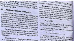
Cardinal utility analysis:- It assumes that, consumer satisfaction can be measured in terms, of cardinal numbers., For ex: we can measure the utility derived from a, shirt , and say this shirt gives me 40 units of utility., It can be classified into, *TU, *MU
Page 7 :
Total utility(TU):- It refers to the total satisfaction, obtained from the consumption of all possible, units of a particular commodity., TUn refers to the total utility derived from, consuming ‘n’ units of a commodity X.
Page 8 :
Marginal utility (MU);- It is the additional utility, derived from the consumption of one more unit of, the given commodity. MU can be calculated as, MU n = TU n- TU n-1
Page 11 :
In the above schedule MU shows a declining, trend as consumer goes on consuming the units., It reaches zero and even becomes negative utility, or dis utility. This is due to law of diminishing, marginal utility.
Page 12 :
Law of diminishing marginal utility;-it states that, as the consumer takes more and more units of a, particular commodity the marginal utility of, additional units goes on diminishing
Page 14 :
In the above diagram we can see that when TU, reaches maximum, MU comes to zero. Afterwards, TU begins to fall and then MU becomes negative.
Page 15 :
Consumption bundle, ●, , Consumption bundle can be defined as the, combination of quantities of two goods that a, consumer can purchase. It can be denoted as x1, and x2., The bundle (5, 10) means 5 units of good1 and 10, units of good 2.
Page 16 :
Consumers budget, ●, , Consumer's budget is the income or amount of, money available for spending on either goods, as the consumer wishes. The consumption, bundle of consumers depends on the prices of, two goods and income of the consumer
Page 17 :
Budget set, ●, , It means the set of all consumption bundle that, a consumer can purchase given his income and, prices of two goods. It contains consumption, bundles less than or equal to his income.
Page 18 :
Budget constraint, ●, , If 'M' is the income of the, consumer P1 & P2 are, prices of two goods then, p1x1 + p2x2 < M is, known as budget, constraint
Page 19 :
Budget line, ●, , A line joining all the, consumption bundles, in which the, consumer spends his, entire income is, known as budget line., p1x1 + p2x2 = M
Page 21 :
Points below and above the budget, line, Any point below the budget, line indicates that the consumer do, not spend his entire income., Any point above the budget, line will certainly be superior to any, point on the budget line. But such a, point would be beyond the income, of the consumer.
Page 22 :
Changes in budget line, ●, , The changes in budget line is that of two, reasons, changes in consumers income, changes in prices of goods
Page 23 :
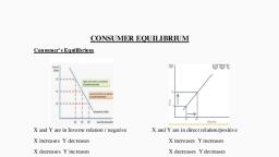
Increase in income ;- when the income of the, consumer increases, the consumer is able to buy, more of two goods and budget line shifts parallel, to rightward.
Page 24 :
Decrease in income;-when consumers income, decreases, he is not able to buy goods with the, same a amount. So the budget line shifts parallel, to leftward.
Page 25 :
Shift in budget line- Income changes
Page 26 :
Change in price of good 1, ●, , ●, , When the price of good 1 increases the new, budget line will move to downward(left) without, change in vertical intercept, When the price of good 1 decreases the new, budget line will move to upward (right) without, change in vertical intercept
Page 28 :
Change in price o good 2, ●, , ●, , When the price of good 2 increases the new, budget line will move to downwards (left), without change in horizontal intercept., When the price of good 2 decreases the new, budget line will move to upward (right) without, change in horizontal intercept
Page 30 :
Shift in budget line – price changes
Page 31 :
Monotonic preference, ●, , Monotonic preference means that a rational, consumer always prefers more of a commodity, as it offers him a higher level of satisfaction., Take a bundle (2,2). this represents 2 units of, good 1 & 2 units of good 2. Certainly a, consumer will prefer this bundle to other, bundles like (1,1) (1,2) (2,1). This preference is, called monotonic preference
Page 32 :
Diminishing rate of substitution, ●, , ●, , The consumers willingness to pay for good 1 in, terms of good 2 would go down or decline. This, is known as diminishing rate of substitution., The rate of substitution between good 1 and, good 2 are called marginal rate of substitution.
Page 33 :
The indifference curve, ●, , An indifference curve shows different bundles which, give the consumer the same level of satisfaction., This analysis was developed by Edge Worth. It was, later perfected by J R Hicks & R G D Allen. It is also, known as the ordinal utility approach.
Page 34 :
Shape of indifference curve, ●, , An indifference curve has a negative slope. If the quantity, of one commodity decreases, the other must increase., The negative slope of the indifference at any one point, is that of marginal rate of substitution [MRS] of the two, commodities. An indifference curve is convex to origin with, diminishing marginal rate of substitution.
Page 35 :
Slope of indifference curve
Page 36 :
Indifference map, ●, , A collection of, indifference curves is, called indifference, map.
Page 37 :
Properties of indifference curve, ✔, ✔, ✔, , Indifference curves do not intersect each other., Indifference curves are convex to the origin., Higher indifference curves represent higher, level of satisfaction.
Page 38 :
IC curves do not intersect with, each other, ●, , If C=A and C=B, then, A should be equal to, B. This is clearly, wrong. Therefore, indifference curve will, not intersect each, other.
Page 39 :
Indifference curves are convex to, origin, ●, , IC curves are convex, to origin, this is due to, diminishing rate of, substitution
Page 40 :
Higher IC curve represents higher, level of satisfaction, ●, , Higher indifference, curves represents higher, levels of satisfaction. In, the diagram IC2 gives, more satisfaction to the, consumer.
Page 41 :
Consumers equilibrium (Optimal, choice of the consumer), ●, , Consumer equilibrium, or optimal choice of, the consumer can be, defined as the point, where the slope of, the indifference curve, and the budget line, are tangent
Page 42 :
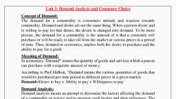
DEMAND, , Demand is desire backed by ability and, willingness to pay for a commodity
Page 43 :
Determinants of demand, ➔, , Price of the commodity, , ➔, , Price of related commodity, , ➔, , Income of the consumer, , ➔, , Taste and preferences of the consumer
Page 44 :
Demand function, Demand function expresses the, relationship between the quantity, demand of a commodity and its, determinants
Page 45 :
Demand function, Demand function expresses the relationship, between the quantity demanded of a, commodity and its determinants, D(x)=f (Px,Pr,Y,T), ●, , Px=price of commodity X, , ●, , Pr=price of related commodity, , ●, , Y =Income of the consumer, , ●, , T =Taste and preference
Page 46 :
Demand for a commodity, Individual demand, ●, Household demand-house hold demand, schedule-house hold demand curve, ●, Market demand-Market demand schedulemarket demand curve, ●
Page 47 :
Individual demand, ●, ●, , It is the quantity of a commodity that an, individual consumer is willing to buy in a given, period of time at a given price
Page 48 :
Household demand, This is the quantity of a commodity that a, household is willing to buy in a given period of, time at a given price
Page 49 :
Household demand schedule, It is a list or table which shows the relationship, between price of the commodity and quantity, demand
Page 50 :
Household demand
Page 51 :
Household demand curve
Page 52 :
Market demand, It is the quantity of a commodity that all, consumers in the market will be willing to buy in, a given period of time at a given price
Page 53 :
Market demand schedule, It is the list or table shows the price, and quantity demanded by all the, consumers in the market.
Page 54 :
Market demand schedule
Page 55 :
Market demand curve, ●, , It is the graphical, representation of, market demand, schedule
Page 56 :
Factors determining market demand, , , Price of a commodity, , , , Price of related commodity, , , , Number of households, , , , Income of the households, , , , Taste and preference, , , , Interest rate, , , , Business condition
Page 57 :
Why does demand curve slopes, downward, , ●, , Income effect, , ●, , Substitution effect, , ●, , Increase in the number of uses, , ●, , Increase in the number of users, , ●, , Low of diminishing marginal utility
Page 58 :
Law of demand, , Other things remaining the, same the quantity demanded of, a commodity varies inversely, with its price
Page 59 :
Exemptions to the law of demand, Giffen goods/inferior goods, ●, Necessities of life, ●, Status symbol goods, ●
Page 60 :
change in demand curve, ●, , Price of the commodity, , ●, , Factors other than price
Page 61 :
Expansion and contraction of, demand, Rise in demand due to, fall in price is known, as expansion of, demand, Fall in demand due to, rise in price is known, as contraction of, demand
Page 62 :
Increase and decrease in demand, Rise in demand due to, factors other than price is, called increase in demand, , Fall in demand due to, factors other than price is, called decrease in, demand
Page 64 :
Degree of price elasticity of, demand, ✔, ✔, ✔, ✔, ✔, , Perfectly elastic demand, Perfectly inelastic demand, Unitary elastic demand, Relatively elastic demand, Relatively inelastic demand
Page 67 :
Unitary elastic demand
Page 70 :
Measurement of price elasticity, Proportionate/percentage method, ●, Total expenditure method, ●, Geometric/point/straight line method, ●
Page 71 :
Percentage method, percentage change in quantity demand, ep =, , Percentage change in price
Page 72 :
Total expenditure method, ●, , ●, , ●, , When, price, , Total expenditure decreases, , price, , Total expenditure increases, , ep>1, , When, price, , Total expenditure increases, , price, , Total expenditure decreases, , When price, , Total expenditure constant, , ep<1, , ep=1
Page 73 :
Geometric /point/straight line, length of lower segment, ep=, a, price, , Length of upper segment, , b, c, d, e, , quantity
Page 75 :
Factors influencing elasticity, ●, , Close substitute, , ●, , Range of price, , ●, , Proportion of income spend on the commodity, , ●, , Extend use of commodity, , ●, , Time horizon, , ●, , Level of income of the consumer, , ●, , Nature of a commodity
Page 76 :
Substitutes and complementaries, ●, , ●, , Substitute goods are those goods which can be used in the, place of another eg: tea or coffee,petrol or diesel,pen or, pencil, Complementary goods are those goods which can be used, together eg:car and petrol, bread and jam, pen and ink