Page 2 : About this Tutorial, An Algorithm is a sequence of steps to solve a problem. Design and Analysis of Algorithm, is very important for designing algorithm to solve different types of problems in the branch, of computer science and information technology., This tutorial introduces the fundamental concepts of Designing Strategies, Complexity, analysis of Algorithms, followed by problems on Graph Theory and Sorting methods. This, tutorial also includes the basic concepts on Complexity theory., , Audience, This tutorial has been designed for students pursuing a degree in any computer science,, engineering, and/or information technology related fields. It attempts to help students to, grasp the essential concepts involved in algorithm design., , Prerequisites, The readers should have basic knowledge of programming and mathematics. The readers, should know data structure very well. Moreover, it is preferred if the readers have basic, understanding of Formal Language and Automata Theory., , Copyright & Disclaimer, Copyright 2017 by Tutorials Point (I) Pvt. Ltd., All the content and graphics published in this e-book are the property of Tutorials Point (I), Pvt. Ltd. The user of this e-book is prohibited to reuse, retain, copy, distribute or republish, any contents or a part of contents of this e-book in any manner without written consent, of the publisher., We strive to update the contents of our website and tutorials as timely and as precisely as, possible, however, the contents may contain inaccuracies or errors. Tutorials Point (I) Pvt., Ltd. provides no guarantee regarding the accuracy, timeliness or completeness of our, website or its contents including this tutorial. If you discover any errors on our website or, in this tutorial, please notify us at
[email protected], , i
Page 3 :
Table of Contents, About this Tutorial .......................................................................................................................................... i, Audience ......................................................................................................................................................... i, Prerequisites ................................................................................................................................................... i, Copyright & Disclaimer ................................................................................................................................... i, Table of Contents........................................................................................................................................... ii, , BASICS OF ALGORITHMS ............................................................................................................. 1, 1., , DAA ─ Introduction ................................................................................................................................. 2, , 2., , DAA ─ Analysis of Algorithms .................................................................................................................. 4, , 3., , DAA ─ Methodology of Analysis .............................................................................................................. 5, Asymptotic Analysis ....................................................................................................................................... 5, Solving Recurrence Equations ....................................................................................................................... 5, Amortized Analysis ........................................................................................................................................ 6, , 4., , DAA ─ Asymptotic Notations & Apriori Analysis ...................................................................................... 8, Asymptotic Notations .................................................................................................................................... 8, O: Asymptotic Upper Bound .......................................................................................................................... 9, Ω: Asymptotic Lower Bound .......................................................................................................................... 9, Ɵ: Asymptotic Tight Bound ............................................................................................................................ 9, O - Notation ................................................................................................................................................. 10, ω – Notation ................................................................................................................................................ 10, Apriori and Apostiari Analysis ...................................................................................................................... 11, , 5., , DAA ─ Space Complexities ..................................................................................................................... 12, What is Space Complexity?.......................................................................................................................... 12, Savitch’s Theorem ....................................................................................................................................... 13, , DESIGN STRATEGIES .................................................................................................................. 14, 6., , DAA ─ Divide & Conquer ....................................................................................................................... 15, , 7., , DAA ─ Max-Min Problem....................................................................................................................... 16, Naïve Method .............................................................................................................................................. 16, Divide and Conquer Approach ..................................................................................................................... 16, , 8., , DAA ─ Merge Sort.................................................................................................................................. 18, , 9., , DAA ─ Binary Search .............................................................................................................................. 20, , 10. DAA ─ Strassen’s Matrix Multiplication ................................................................................................. 22, Naïve Method .............................................................................................................................................. 22, Strassen’s Matrix Multiplication Algorithm ................................................................................................. 22, 11. DAA ─ Greedy Method .......................................................................................................................... 24, , ii
Page 4 :
12. DAA ─ Fractional Knapsack .................................................................................................................... 25, Knapsack Problem ....................................................................................................................................... 25, Fractional Knapsack ..................................................................................................................................... 26, 13. DAA ─ Job Sequencing with Deadline .................................................................................................... 29, 14. DAA ─ Optimal Merge Pattern ............................................................................................................... 31, 15. DAA ─ Dynamic Programming ............................................................................................................... 34, 16. DAA ─ 0-1 Knapsack .............................................................................................................................. 35, Dynamic-Programming Approach ............................................................................................................... 36, 17. DAA ─ Longest Common Subsequence .................................................................................................. 38, , GRAPH THEORY......................................................................................................................... 41, 18. DAA ─ Spanning Tree ............................................................................................................................. 42, Minimum Spanning Tree ............................................................................................................................. 42, Prim’s Algorithm .......................................................................................................................................... 43, 19. DAA ─ Shortest Paths ............................................................................................................................ 45, Dijkstra’s Algorithm ..................................................................................................................................... 45, Bellman Ford Algorithm ............................................................................................................................... 47, 20. DAA ─ Multistage Graph ........................................................................................................................ 51, 21. DAA ─ Travelling Salesman Problem ...................................................................................................... 53, 22. DAA ─ Optimal Cost Binary Search Trees ............................................................................................... 56, , HEAP ALGORITHMS ................................................................................................................... 59, 23. DAA ─ Binary Heap ................................................................................................................................ 60, 24. DAA ─ Insert Method............................................................................................................................. 63, 25. DAA ─ Heapify Method.......................................................................................................................... 65, 26. DAA ─ Extract Method........................................................................................................................... 66, , SORTING METHODS .................................................................................................................. 68, 27. DAA ─ Bubble Sort ................................................................................................................................. 69, 28. DAA ─ Insertion Sort .............................................................................................................................. 71, 29. DAA ─ Selection Sort ............................................................................................................................. 73, 30. DAA ─ Quick Sort ................................................................................................................................... 76, iii
Page 5 :
31. DAA ─ Radix Sort ................................................................................................................................... 78, , COMPLEXITY THEORY................................................................................................................ 80, 32. DAA ─ Deterministic vs. Nondeterministic Computations ..................................................................... 81, Deterministic Computation and the Class P ................................................................................................ 81, Nondeterministic Computation and the Class NP ....................................................................................... 81, 33. DAA ─ Max Cliques ................................................................................................................................ 83, 34. DAA ─ Vertex Cover ............................................................................................................................... 85, 35. DAA ─ P and NP Class ............................................................................................................................ 88, 36. DAA ─ Cook’s Theorem .......................................................................................................................... 90, 37. DAA ─ NP Hard & NP-Complete Classes ................................................................................................. 92, 38. DAA ─ Hill Climbing Algorithm ............................................................................................................... 94, Hill Climbing ................................................................................................................................................. 94, Problems of Hill Climbing Technique ........................................................................................................... 95, Complexity of Hill Climbing Technique ........................................................................................................ 95, Applications of Hill Climbing Technique ...................................................................................................... 96, , iv
Page 6 :
Basics of Algorithms, , 5
Page 7 :
1. DAA ─ Introduction, , An algorithm is a set of steps of operations to solve a problem performing calculation, data, processing, and automated reasoning tasks. An algorithm is an efficient method that can be, expressed within finite amount of time and space., An algorithm is the best way to represent the solution of a particular problem in a very simple, and efficient way. If we have an algorithm for a specific problem, then we can implement it, in any programming language, meaning that the algorithm is independent from any, programming languages., , Algorithm Design, The important aspects of algorithm design include creating an efficient algorithm to solve a, problem in an efficient way using minimum time and space., To solve a problem, different approaches can be followed. Some of them can be efficient with, respect to time consumption, whereas other approaches may be memory efficient. However,, one has to keep in mind that both time consumption and memory usage cannot be optimized, simultaneously. If we require an algorithm to run in lesser time, we have to invest in more, memory and if we require an algorithm to run with lesser memory, we need to have more, time., , Problem Development Steps, The following steps are involved in solving computational problems., , , Problem definition, , , , Development of a model, , , , Specification of an Algorithm, , , , Designing an Algorithm, , , , Checking the correctness of an Algorithm, , , , Analysis of an Algorithm, , , , Implementation of an Algorithm, , , , Program testing, , , , Documentation, , Characteristics of Algorithms, The main characteristics of algorithms are as follows:, 6
Page 8 :
, , Algorithms must have a unique name, , , , Algorithms should have explicitly defined set of inputs and outputs, , , , Algorithms are well-ordered with unambiguous operations, , , , Algorithms halt in a finite amount of time. Algorithms should not run for infinity, i.e.,, an algorithm must end at some point, , Pseudocode, Pseudocode gives a high-level description of an algorithm without the ambiguity associated, with plain text but also without the need to know the syntax of a particular programming, language., The running time can be estimated in a more general manner by using Pseudocode to, represent the algorithm as a set of fundamental operations which can then be counted., , Difference between Algorithm and Pseudocode, An algorithm is a formal definition with some specific characteristics that describes a process,, which could be executed by a Turing-complete computer machine to perform a specific, task. Generally, the word "algorithm" can be used to describe any high level task in computer, science., On the other hand, pseudocode is an informal and (often rudimentary) human readable, description of an algorithm leaving many granular details of it. Writing a pseudocode has no, restriction of styles and its only objective is to describe the high level steps of algorithm in a, much realistic manner in natural language., For example, following is an algorithm for Insertion Sort., , Algorithm: Insertion-Sort, Input: A list L of integers of length n, Output: A sorted list L1 containing those integers present in L, Step 1: Keep a sorted list L1 which starts off empty, Step 2: Perform Step 3 for each element in the original list L, Step 3: Insert it into the correct position in the sorted list L1., Step 4: Return the sorted list, Step 5: Stop, Here is a pseudocode which describes how the high level abstract process mentioned above, in the algorithm Insertion-Sort could be described in a more realistic way., for i ← 1 to length(A), x ← A[i], j ← i, 7
Page 9 :
while j > 0 and A[j-1] > x, A[j] ← A[j-1], j ← j - 1, A[j] ← x, In this tutorial, algorithms will be presented in the form of pseudocode, that is similar in many, respects to C, C++, Java, Python, and other programming languages., , 8
Page 10 :
2. DAA ─ Analysis of Algorithms, , In theoretical analysis of algorithms, it is common to estimate their complexity in the, asymptotic sense, i.e., to estimate the complexity function for arbitrarily large input. The term, "analysis of algorithms" was coined by Donald Knuth., Algorithm analysis is an important part of computational complexity theory, which provides, theoretical estimation for the required resources of an algorithm to solve a, specific computational problem. Most algorithms are designed to work with inputs of arbitrary, length. Analysis of algorithms is the determination of the amount of time and space resources, required to execute it., Usually, the efficiency or running time of an algorithm is stated as a function relating the input, length to the number of steps, known as time complexity, or volume of memory, known as, space complexity., , The Need for Analysis, In this chapter, we will discuss the need for analysis of algorithms and how to choose a better, algorithm for a particular problem as one computational problem can be solved by different, algorithms., By considering an algorithm for a specific problem, we can begin to develop pattern, recognition so that similar types of problems can be solved by the help of this algorithm., Algorithms are often quite different from one another, though the objective of these, algorithms are the same. For example, we know that a set of numbers can be sorted using, different algorithms. Number of comparisons performed by one algorithm may vary with, others for the same input. Hence, time complexity of those algorithms may differ. At the same, time, we need to calculate the memory space required by each algorithm., Analysis of algorithm is the process of analyzing the problem-solving capability of the, algorithm in terms of the time and size required (the size of memory for storage while, implementation). However, the main concern of analysis of algorithms is the required time or, performance. Generally, we perform the following types of analysis:, , , Worst-case: The maximum number of steps taken on any instance of size a., , , , Best-case: The minimum number of steps taken on any instance of size a., , , , Average case: An average number of steps taken on any instance of size a., , , , Amortized: A sequence of operations applied to the input of size a averaged over, time., , 9
Page 11 :
To solve a problem, we need to consider time as well as space complexity as the program, may run on a system where memory is limited but adequate space is available or may be, vice-versa. In this context, if we compare bubble sort and merge sort. Bubble sort does, not require additional memory, but merge sort requires additional space. Though time, complexity of bubble sort is higher compared to merge sort, we may need to apply bubble, sort if the program needs to run in an environment, where memory is very limited., , 10
Page 12 :
3. DAA ─ Methodology of Analysis, , To measure resource consumption of an algorithm, different strategies are used as discussed, in this chapter., , Asymptotic Analysis, The asymptotic behavior of a function 𝒇(𝒏) refers to the growth of 𝒇(𝒏) as n gets large., We typically ignore small values of n, since we are usually interested in estimating how slow, the program will be on large inputs., A good rule of thumb is that the slower the asymptotic growth rate, the better the algorithm., Though it’s not always true., For example, a linear algorithm 𝒇(𝒏) = 𝒅 ∗ 𝒏 + 𝒌 is always asymptotically better than a, quadratic one, 𝒇(𝒏) = 𝒄. 𝒏𝟐 + 𝒒., , Solving Recurrence Equations, A recurrence is an equation or inequality that describes a function in terms of its value on, smaller inputs. Recurrences are generally used in divide-and-conquer paradigm., Let us consider 𝑻(𝒏) to be the running time on a problem of size n., If the problem size is small enough, say 𝒏 < 𝒄 where c is a constant, the straightforward, solution takes constant time, which is written as Ɵ(𝟏). If the division of the problem yields a, 𝒏, number of sub-problems with size ., 𝒃, , To solve the problem, the required time is 𝒂. 𝑻(𝒏/𝒃). If we consider the time required for, division is 𝑫(𝒏) and the time required for combining the results of sub-problems is 𝑪(𝒏), the, recurrence relation can be represented as:, 𝑻(𝒏) = {, , 𝜽(𝟏) 𝒊𝒇 𝒏 ≤ 𝒄, 𝒏, 𝒂𝑻 ( ) + 𝑫(𝒏) + 𝑪(𝒏), 𝐨𝐭𝐡𝐞𝐫𝐰𝐢𝐬𝐞, 𝒃, , A recurrence relation can be solved using the following methods:, , , Substitution Method ─ In this method, we guess a bound and using mathematical, induction we prove that our assumption was correct., , , , Recursion Tree Method ─ In this method, a recurrence tree is formed where each, node represents the cost., , 11
Page 13 :
, , Master’s Theorem ─ This is another important technique to find the complexity of a, recurrence relation., , Amortized Analysis, Amortized analysis is generally used for certain algorithms where a sequence of similar, operations are performed., , , Amortized analysis provides a bound on the actual cost of the entire sequence, instead, of bounding the cost of sequence of operations separately., , , , Amortized analysis differs from average-case analysis; probability is not involved in, amortized analysis. Amortized analysis guarantees the average performance of each, operation in the worst case., , It is not just a tool for analysis, it’s a way of thinking about the design, since designing and, analysis are closely related., , Aggregate Method, The aggregate method gives a global view of a problem. In this method, if n operations takes, worst-case time 𝑻(𝒏) in total. Then the amortized cost of each operation is 𝑻(𝒏)/𝒏. Though, different operations may take different time, in this method varying cost is neglected., , Accounting Method, In this method, different charges are assigned to different operations according to their actual, cost. If the amortized cost of an operation exceeds its actual cost, the difference is assigned, to the object as credit. This credit helps to pay for later operations for which the amortized, cost less than actual cost., If the actual cost and the amortized cost of ith operation are 𝒄𝒊 and 𝒄̂𝒊 , then, 𝒏, , 𝒏, , ∑ 𝒄̂𝒊 ≥ ∑ 𝒄𝒊, 𝒊=𝟏, , 𝒊=𝟏, , Potential Method, This method represents the prepaid work as potential energy, instead of considering prepaid, work as credit. This energy can be released to pay for future operations., If we perform 𝒏 operations starting with an initial data structure 𝑫𝟎 . Let us consider, 𝒄𝒊 as the, actual cost and 𝑫𝑖 as data structure of ith operation. The potential function ф maps to a real, number ф(𝑫𝒊 ), the associated potential of 𝑫𝒊 . The amortized cost 𝒄̂𝒊 can be defined by, 𝒄̂𝒊 = 𝒄𝒊 + ф(𝑫𝒊 ) − ф(𝑫𝒊−𝟏 ), 12
Page 14 :
Hence, the total amortized cost is, 𝒏, , 𝒏, , 𝒏, , ∑ 𝒄̂𝒊 = ∑(𝒄𝒊 + ф(𝑫𝒊 ) − ф(𝑫𝒊−𝟏 )) = ∑ 𝒄𝒊 + ф(𝑫𝒏 ) − ф(𝑫𝟎 ), 𝒊=𝟏, , 𝒊=𝟏, , 𝒊=𝟏, , Dynamic Table, If the allocated space for the table is not enough, we must copy the table into larger size, table. Similarly, if large number of members are erased from the table, it is a good idea to, reallocate the table with a smaller size., Using amortized analysis, we can show that the amortized cost of insertion and deletion is, constant and unused space in a dynamic table never exceeds a constant fraction of the total, space., In the next chapter of this tutorial, we will discuss Asymptotic Notations in brief., , 13
Page 15 :
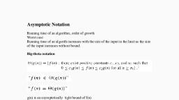
4. DAA ─ Asymptotic Notations & Apriori Analysis, , In designing of Algorithm, complexity analysis of an algorithm is an essential aspect. Mainly,, algorithmic complexity is concerned about its performance, how fast or slow it works., The complexity of an algorithm describes the efficiency of the algorithm in terms of the, amount of the memory required to process the data and the processing time., Complexity of an algorithm is analyzed in two perspectives: Time and Space., , Time Complexity, It’s a function describing the amount of time required to run an algorithm in terms of the size, of the input. "Time" can mean the number of memory accesses performed, the number of, comparisons between integers, the number of times some inner loop is executed, or some, other natural unit related to the amount of real time the algorithm will take., , Space Complexity, It’s a function describing the amount of memory an algorithm takes in terms of the size of, input to the algorithm. We often speak of "extra" memory needed, not counting the memory, needed to store the input itself. Again, we use natural (but fixed-length) units to measure, this., Space complexity is sometimes ignored because the space used is minimal and/or obvious,, however sometimes it becomes as important an issue as time., , Asymptotic Notations, Execution time of an algorithm depends on the instruction set, processor speed, disk I/O, speed, etc. Hence, we estimate the efficiency of an algorithm asymptotically., Time function of an algorithm is represented by 𝐓(𝐧), where n is the input size., Different types of asymptotic notations are used to represent the complexity of an algorithm., Following asymptotic notations are used to calculate the running time complexity of an, algorithm., , , O: Big Oh, , , , Ω: Big omega, , , , Ɵ: Big theta, , , , o: Little Oh, , , , ω: Little omega, 14
Page 19 :
End of ebook preview, If you liked what you saw…, Buy it from our store @ https://store.tutorialspoint.com, , 18