Page 1 :
SEM IV, , UNIT II, , 2022, , **Statistical Quality Control**, Meaning:, S.Q.C. means planned collection & effective use of data for studying causes of variations in quality either as, between processes, procedures, materials, machines etc. or over periods of time. By statistical quality, control, we mean the various statistical methods used for the maintenance of the quality in manufactured, product., Purpose of SQC:, 1) To provide a basis for a better understanding of the variations that exists in quality characteristics., 2) To help directly or indirectly to improve quality., 3) To help in separating the assignable causes from the chance causes., 4) Better uniformity of quality., 5) Better utilization of raw materials., 6) More efficient use of equipment., 7) Less scrap and rework, hence lowering costs., 8) Better inspection., 9) Improved producer-consumer relations., Quality of Product:, Quality product means good or excellent product. In industry, a quality product is one that fulfills, customer’s expectations. These expectations are based on the intended use and the selling price of the, product. In other words, quality must be judged in customer satisfaction. Quality means fitness for use., Quality is inversely proportional to variability. Quality improvement is the reduction of variability in, processes and products. Quality of a product is related with the following:, i) Quality of material: Material of good quality will result in smooth processing thereby reducing the waste, & increasing the output. It will also give better finish of end products., ii) Quality of manpower: Trained & qualified personnel will give increased efficiency due to the better, quality production through the application of skills & also reduce production cost & waste., iii) Quality of machines: Better quality equipment will result in efficient working due to lack or scarcity of, breakdowns & thus reduce the cost of defectives., iv)Quality of management: A good management is imperative for increase in efficiency, harmony in, relations, growth of business & markets., Types of Control:, 1) Process Control: Process controls are quality systems based on preventing defects by controlling and, monitoring manufacturing processes. Because no defective product is produced, these processes can achieve, much higher quality levels. Processes must be rigorously characterized, understood, and controlled for this, system to be effective. Here we want to ensure that the proportion of defective items in the manufactured, product is not too large. This is achieved through the technique of control charts., 2) Product Control: Product controls are quality systems that focus on sorting and isolating defective, product. Because the process generates defective product, efforts are made to identify, sort, and segregate, them. Management also must be prepared to accept the greater costs that come with a quality system, founded on product controls. In order to have quality system based on controlling product, robust systems, for material control, calibration, maintenance, and rework (as applicable) are required., , 1, , B. Sc. II, , map_stats@yahoo.co.in

Page 2 :
SEM IV, , UNIT II, , 2022, , Causes of variation:, Chance Causes, These causes are natural., These cannot be detected or predicted., , Assignable Causes, These are not natural., These can be detected & removed from, production process., These causes are called allowable causes., These are called preventable causes., Variation due to these causes is small or Variation due to these causes are high & they, negligible., cannot be tolerated., Chance variations behave in a random manner These are manmade causes., & beyond the control of human hand., Chance causes cannot be identified., These can be identified., It is due to slight variation in electric current It is due to inferior raw material, improper, supplied to the machine., machine setting, wrong handling of machine,, defect in machine, inexperienced worker,, negligence of operators etc., , 01, 02, 03, 04, 05, 06, 07, , SHEWHART CONTROL CHART:, Control chart are most commonly used methods of statistical process control which monitors the stability of, a process. It is a powerful graphical tool of detecting assignable causes of variation. This technique was, developed by Dr. Walter A. Shewhart in 1924.Control chart consists of three lines: a) a central line b) upper, control limit c) lower control limit. The central line denotes the expected value of the statistics such as, length, diameter etc. of a product. Then the line corresponding to the limits prescribed are drawn. One lying, above the central line and indicating the upper limit of the statistic is called the upper control limit. The, other line lying below the central line and indicating the lower limit of the statistic is called the lower control, limit., Y↑, UCL, AVG, LCL, , Outline of a control chart., OUT OF CONTROL, ↑, 3-Sigmas, ↓, ↑, 3-Sigmas, ↓, OUT OF CONTROL, X→, SAMPLE ( SUB-GROUP) NUMBER, , Construction: While plotting the chart, take sample numbers on x-axis & the corresponding statistic on yaxis. The first thing to plot is the center line. Next we need an estimate of σ calculated for each subgroup., The control limits are then plotted at 3-σ above & below the center line for each subgroup. Then plot the, data points on the chart by indicating a dot for each point. Those points who felled beyond these limits can, be encircled., Working of the chart: If all the points plotted on the chart are within the limits without exhibiting any, specific pattern, then the process is said to be in a state of control. There is nothing to worry as in such a, case variation between samples is attributed to chance. It is only when any observed point falls outside the, control limits, it is considered to be a danger signal indicating that some assignable cause has crept in which, must be identified & eliminated., 2, , B. Sc. II, , map_stats@yahoo.co.in

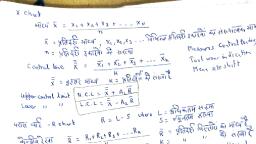
Page 3 :
SEM IV, , UNIT II, , 2022, , Out of Control: The situation in which a plotof data falls outside presetcontrol limits., Theoretical Basis: Let θ be the population parameter under considerations & let t=t(x1, x2, …xn), a function, of the sample observations x1,x2,..,xn be the corresponding statistic., Let E (t) =μ t& V (t) = σ2t, If t is normally distributed, then, P [│t-E (t) │< 3σ t] = 0.9973, →, P [│t-μ t│< 3σ t] = 0.9973, In other words, the probability that a random value of t goes outside the limits μ t ± 3σ t is 0.0027, which is, very small. Hence, if t is normally distributed, the limits of variation should be between μ t+ 3 σ t &, μt -3 σ t which are termed respectively the U.C.L. & L.C.L., Lack of control situation: A control chart can be indicating an out of control condition even though no, single point exhibits nonrandom or systematic behavior., A) If all the points of the chart are showing random pattern with UCL and LCL, it indicates process is, governed by chance cause of variation alone., Therefore, adjustment to the process is not required and process is allowed to continue., B) If both, and R chart shows nonrandom pattern of points, eliminate assignable causes from R-chart, alone. This may eliminate assignable causes from, chart also., C) A cyclic pattern of points may be due to maintenance schedule., D) A mixture is indicated when the plotted points tends to fall near or slightly outside the control limits,, with relatively few points near the central line. It is due to frequent adjustment of the process., E) A shift in process level may result from the introduction of new workers, methods, raw material or, machine; a change in the inspection method or standards., F) A trend or continuous movement in one direction of control chart points may be due to settling or, separation of the components of a mixture, in chemical processes., G) Stratification or a tendency for the points to cluster artificially around the central line is an indication of, incorrect observations provided to plot the control chart., Use of control chart:, 1)It helps to monitor, control & improve process performance over time by studying variations & its source., 2) It provides a tool for ongoing control of a process., 3) It differentiates chance causes from assignable causes of variation., 4) It helps to improve a process to perform consistently and predictably to achieve higher quality, lower cost, & higher effective capacity., 5) It serves as a common language for discussing process performance., TYPES OF CONTROL CHARTS:, A) CONTROL CHART FOR VARIABLES:, Definition: & R charts:Aquantitative characteristic which can be measured numerically is called a, variable. For example, length, diameter etc. For these variates, we may be interested in controlling their, mean or the range of variation. These charts are useful in detecting assignable causes of variation in the, a)average- related to machine setting &, b)range- related to negligence on the part of the operator., Let X be quality characteristic of interest which follows normality i.e. X →N (μ, σ2), →N (μ, σ2 / n), E ( ) = μ and S.E. ( ) = σ / √ n, When μ is unknown, its estimate, , 3, , is used, since E (, , B. Sc. II, , ) = μ where Sample mean =, , =, , ∑, , 𝑖, , 𝑘, , map_stats@yahoo.co.in

Page 4 :
SEM IV, UNIT II, 2022, Also from sampling distribution of range, E(R) = d2 σ, d2 is a constant depending on the sample size → =, ∑𝑅, d2*σ → σ =, / d2 and S.E. (R) = d3* σ where sample range =, = 𝑘 𝑖 where k = # of samples, The 3-σ control limits for, -chart are given byE ( ) ± 3 S.E. ( ) →, ±3σ/√n→, → ± A2, where A2 = 3/ d2 √n, , C.L. =, , ,, , UCL =, , + A2, , ,, , LCL=, , ±3, , / d2 * 1 / √n →, , ± (3/ d2 √n), , - A2, , Since d2 is a constant depending on n, A2 also depends only on n and its values have been computed and, tabulated for different values of n from 2 to 20., The 3-σ control limits for R-chart are given byE (R) ± 3 S.E. (R) →, ± d3 * σR →, ±3, d3 / d2 →, (1± 3 d3/ d2), →, (1 ±3 k) →, (1 + 3 k) or (1 – 3 k) → D4*, or D3 *, where k = d3/ d2,, D4 = 1 + 3k and D3 = 1- 3k, ., , C.L. =, , ,, , UCL = D4*, , ,, , LCL= D3 *, , ., , The values of D4 and D3 have been tabulated for different values on n from 2 to 20., Working: Same as discussed in shewhart’s control chart., Revised Control Limits for, & R chart: It is essential to revise control limits frequently on the basis of, change of operator, change of machine, setting of machine etc. To revise control limits following step are to, be followed., 1) When R chart is out of control eliminate the points showing out of control and re-compute ., 2) Use this value to recompute control limits for, & R chart., 3) This will tighten the control limits on both charts, continue this till both R and, chart shows in control., Estimate of process s. d.: There is a well-known relationship between the range of a sample from a normal, distribution and the s.d. of that distribution. The r.v. w= R / σ is called the relative range. The parameters of, the distribution of w are a function of the sample size n. Again, E (w) = d2., Consequently, an estimator of σ is = R / d2. Again, E (w) = E(R) / σ → d2 =, / σ → σ = / d2., , B) CONTROL CHART FOR ATTRIBUTES:, Many quality characteristics cannot be represented numerically are called attributes., The difference between defect and defective:, Sr No, 01, , defect, , defective, , Defect means failing to deliver what the, customer/client wants., , 02, , A product shows one or more defect(s)., , 03, 04, 05, 06, , It is also called as non-conformity., For construction, Poisson distribution can be used., Here we can use C –chart., , Control charts involving counts can be either for, the total number of nonconformities (defects) for, the sample of inspected units, or for the average, number of defects per inspection unit., , 4, , B. Sc. II, , Defective means failing of the entire, product/service to meet the required criterion., A product is defective. Every defective contains, at least one or more defect., It is also called as nonconforming unit., For construction, binomial distribution can be used., Here we can use np or p-chart., The classification of items is either defective or, nondefective., , map_stats@yahoo.co.in

Page 5 :
SEM IV, , UNIT II, , 2022, , i) Control chart for proportion or fraction non-conforming (defective): p-chart:, Definition: It is the ratio of the number of nonconforming items in the population to the total number of, items in that population. In this case, classification of item as defective or non-defective., The objective of this chart is to evaluate the quality of items., If d is the no of defectives in a sample of size n, then the sample proportion defective is p=d/n., Hence, d →B (n, p) E (d) =n p & V (d) =n p q, q=1-p. the sample fraction non-conforming = d / n., E (d), 𝑛𝑃, The mean and variance of is E (p) =E (d/n) = 𝑛 = 𝑛 = P, V (p) =V (d/n) =, , V (d), 𝑛2, , =, , 𝑛𝑝𝑞, 𝑛2, , =, , 𝑝𝑞, , S.E. (p) = √p q/n, , 𝑛, , When p is unknown, the statistic, estimates the unknown fraction nonconforming p., Let p = d / n →, = / n = Σ di / nk,, =1The 3-σ control limits for p-chart are given byE (p) ± 3 S.E. (p) →, , ±3√, , C.L. = , UCL =, , /n, , +3√, , -3√, , / n, LCL=, , /n, , Since, p can’t be negative, if LCL given by above formulae comes out to be negative, it is regarded as zero, i.e. LCL = 0., Construction: While plotting the chart, take sample numbers on x-axis & the corresponding statistic p on yaxis. Draw the control limits for p. The CL is drawn by using solid horizontal line and the UCL & LCL is, drawn by using dotted horizontal line. The points may be indicated on the chart by a dot and the points, above the limits can be shown by using encircling the dot., Working: Same as discussed in shewhart’s control chart., Revised Control Limits for p chart: The control limits defined above are trial control limits. The graph of, pi versus trial control limits are plotted to test whether the process was in control. Any point that exceeds the, trial control limits should be investigated. If assignable causes for these points are discovered, they should, be discarded & new trial control limits determined., ii) Control chart for number of defects per unit (c-chart):, Definition: Any instance of articles lack of conformity to specification is a defect., Let us consider an assembled product such as a microcomputer. The opportunity for the occurrence of any, given defect may be quite large. However, the probability of occurrence of a defect in any one arbitrarily, chosen spot is likely to be very small. In such a case, the incidence of defects might be modeled by, a Poisson distribution., Suppose, X →P(C), x= 0, 1, 2,…….where X= no of nonconformities & C > 0 is a parameter of Poisson, distribution. E(X) = C, V(X) = C, S.E. (X) = √C, Thus 3-σ control limits for C-chart are given by-E (X) ± 3 S.E. (X) → C ± 3 √v(C) → C ± 3√C, When C is unknown, it may be estimated as the observed average no of nonconformities in a preliminary, sample of inspection units, say, , where, , =, , ∑ 𝐶𝑖, 𝑘, , It can be seen that, is an unbiased estimate of C., Thus 3-σ control limits for C-chart are given byE (X) ± 3 S.E. (X) →, ± 3 √V ( ) →, ± 3√, C.L. =, , 5, , , UCL =, , +3√, , , LCL =, , - 3√, , B. Sc. II, , map_stats@yahoo.co.in

Page 6 :
SEM IV, UNIT II, 2022, Since, C can’t be negative, if LCL given by above formulae comes out to be negative, it is regarded as zero, i.e. LCL = 0., Construction: While plotting the chart, take sample numbers on x-axis& the corresponding statistic C on yaxis. Draw the control limits for C. The CL is drawn by using solid horizontal line and the UCL & LCL is, drawn by using dotted horizontal line. The points may be indicated on the chart by a dot and the points, above the limits can be shown by using encircling the dot., Working: Same as discussed in shewhart’s control chart., Revised Control Limits for c chart: Same as above given in p chart. Only replace p by c., Real life situation: 1) Accident Statistics (both industrial & highway), 2) Chemical Laboratories, 3) In epidemiology., , This resource material is prepared by Prof Milind Patil of Department of Statistics of Dr. Ghali College,, Gadhinglaj for internal circulation purpose only., , HAPPY LEARNING, , 6, , B. Sc. II, , map_stats@yahoo.co.in