Page 1 :
—, _, , 1. Introduction, , , , 1th rmodynamics mainly deals with the study of the processes which begain and end with, saaical the, casi, , “state through the intermediate states of a process, which may be non-equilibrium., sguilbium s, , brium state can only be realized only in the man-made systems. however on the other hand, all, , An aquilibriut ses are irreversible processes which take place in open systems. The time-invariant of these, cece isa steady state. not the equilibrium state. Steady state is, infect, the limiting case of, bes Tee when the fluxes like mass flow of heat. electricity etc. arising from the environment stop to, a eiendile thermodynamics is also known as non-equilibrium thermodynamics., , , , 2, Thermodynamics of Non-equilibrium State, , Classical thermodynamics is conerned with the detailed study of the systems which are in equilibrium., However, many transport processes (involving flow of different types of quantities) may take place in the, , tem which may be irreversible and the system may not be in equilirbium with respect to these quantities. A, few examples of such transport phenomena include flow (conduction) of heat along a metal bar whose ends, ae kept at a fixed but at different temperatures, the development of heat when an electric current flows, through a metallic conductor. diffusion of a solid or a fluid across a concentration gradient etc., , , , , , The branch of science dealing with the study of thermodynamic properties of the systems which are not in, equilibrium and involve transport processes which are irreversible is termed as non-equilibrium or, ineversible thermodynamics or thermodynamics for irreversible processes., h order to develop the general theory for the irreversible processes, some additional postulates, mela) have tobe introduced. These postulates are solely applicable only when the system is “not too, ; im equilibrium i.e., to the states which are close to equilibrium. Hence irreversible thermodynamics is, Pplicable to those systems which are Not too far from equilibrium, T equilibrium does ist. i ;, Ges not exist, it becomes necessary to red i i, , : : : efine the t, , ibbs function and entropy. It is assumed that : ” Sen S ee: SRS ae, Raa apes, “Temperature (T), , , Pressure (P), i oc is :, , | non-equilibrisn @ibiepend ten en eee Gibbs function (G) and entropy (S) for a cell in, Sxactly in the same manner as in an aquillariita ten Br, Te cuass Units frida) thenplesalar specie, | non-equilibrium is treated exactly in the same rane (erie other words, each cell Gd Sister, | ©duilibrium exists in each of these cell m, , o anner (statistically as well as thermodynamically) as, | This is also termed as the assumption of lo., ——, , cal equilibrium,, , Scanned with CamScanner

Page 2 :
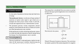
j tem in equilibrium is maximum, H, |, tropy of an isolated sys ximurn, Henco ‘, The eropy wil increase but may not decreasei.e., equilibrium lies in att & ae, is termed “entropy production . sr, The concept of entropy producti, , follows. It is known that oN, as2 22 ating,, T a, t, or which can be rearranged in the form a :, dS-—~20, T, The quantity on the left is greater than or equal to zero. So we may write, dQ, dS — a do, , Where do “iil be either zero or positive., If it is assumed that the system is in contact with a reservoir at T and a quantity, , system, then a quantity ‘- dQ’ flows in the reservoir. If the quantity ‘— dQ’ is oneal \ om, reservoir, then the entropy change of the reservolr Is erred Teversy fi, = dQ a, dS=-—= 1, , T, , So that the eq. (1) can be written as, , dS+dS,,, = do, The quantity do refers to the entropy increase of the system plus that of the surroundings (the teseng:, do is called the entropy production of the process. For an irreversible process the entron ail, positive while for a reversible process, the entropy production is zero. Y Produ, Let us now derive the exact expressions for the entropy production accompanying the flow of heatart|, matter (which are irreversible processes) for the system not in equilibrium but very close to the equi, , 3.1 Entropy Production in Heat Flow, , Suppose our system is having a metal rod. Consider two regions of the metal, rod maintained at different temperatures T, and To i.e., each region is, isothermal. This can be achieved by allowing the heat to enter one region and, leave the other region at the same rate., , If bq, refers to the amount of heat that enters the region at T, per unit time and, 8qz is the amount of heat that leaves the region at T per unit time, then, , , , . . 8q, . . 5q |, Entropy change in region 1 = Tr, and entropy change in region 2= Tr Fig. 1 i, But as each of the regions 1 and 2 is isothermal, therefore we must have, 8q, = — 542 :, Net entropy change accompanying the irreversible flow of heat will be give? Uy, 1 —T, dS, = 8q Jeet = 6q2 Te 2, Ty T2 TyT2 7, , ay stil 2, ee onutiny (2) we see that Ty > Tj, (dS),, > 0. Even if T) > T2 dSyr wil in, q. (5) in the parentheses is < 0. Since, dq, will be < 0. The entropy Pt, , when thermal equilibrium is established that is, when, , Ty =T, —— |, , Scanned with CamScanner

Page 3 :
ie, , , , , , , , , , EA] ‘ ety Be sue:, / Nom roduction per unit time, o is gi, 7" 6) the entropy P Gard given by, fo - Sua (2-2),0, dt dt \T, Tz (1), tropy production is the product of t ;, ws that rate ofen product of two terms th, ett" mer of state functions i.e. 1) this aiff at isthe rate of heat transter, i 1.4) fe ;, | a and the difference 7, Ts rence of state function can be considered, di ses or the deriving force for the heat transfer whi :, the yoscopic Ca¥ uence of the deriving force nsfer which can be considered as a flux or, a flow ora conseq| 3, ttl . ., , entropy production in Matter Flow, 42 «or the flow ofén moles of some component of the matter (or of Tat, ae from one region of temperature T,, where the chemical ty May 2» Ha, coil toa second region where the temperature isT, and the !, u cis ', Focal potential is flo: 3——, : en matter (fluid) flows from a cooler region to the hotter region, ‘, ee the heat content of the substance increases say be dH per \, wees orrepresented as H but also a heat effect takes place when the ;, ‘ia enters the surface of the barrier and passes into the interior. This Barrier, may be thought of as primarily the heat of solution. This quantity is, called the heat of transfer and is written as Q: per mole. Fig. 2 : Flow of matter from, one region to another, , Now the partial molal entropy of a system (entropy pet mole) having, d chemical potential 1. and maintained a, , partial molal enthalpy H an t temperature T is given by, , gf ...(8), T T, Taking the heat of transfer (Q’) also into consideration the above equation becomes, H+Q, pee) E (9), , , , S=, T T, , DO - *, ., he sum HT + Q’ must be same whether we are considering region, , According to first law of thermodynamics, t, , , , lor region 2., Thus the partial molal entropy of region | is, 5= H+Q\_ th ...(10), T T2, and the partial molal entropy of region 2 is, 5, -(Re _b2 (1, To To, Increase of entropy per mole transfer of matter from region 1 to region 2 will be, B-5,-5,-(H- te] + Ait 12, T Tp ln h ~, Entropy increase for the transfer of 6n moles will be given by, dS, =f (ta) 11, rr —— + Q*)} — -—, 1) Ts Q*) TT; dS, or for infinitesimal differences, as before, we can write, dS, ~an|-a(# 7 1, i rT + +ond(2)| ...(14, , , , Scanned with CamScanner