Page 1 :
Sampling, PAM- Pulse Amplitude Modulation, (continued), EELE445-14, Lecture 14, , Sampling, , Properties will be looking at for:, •Impulse Sampling, •Natural Sampling, •Rectangular Sampling, , 1

Page 4 :
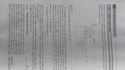
Impulse Sampling, The spectrum of the impuse sampled signal is the spectrum of the, unsampled signal that is repeated every fs Hz, where fs is the, sampling frequency or rate (samples/sec). This is one of the, basic principles of digital signal processing., Note:, This technique of impulse sampling is often used to, translate the spectrum of a signal to another frequency band that, is centered on a harmonic of the sampling frequency, fs., If fs>=2B, (see fig 2-18), the replicated spectra around, each harmonic of fs do not overlap, and the original spectrum can, be regenerated with an ideal LPF with a cutoff of fs/2., , Impulse Sampling, Undersampling and aliasing., , 4

Page 5 :
Natural Sampling, Generation of PAM with natural sampling (gating)., , Natural Sampling, , Duty cycle =1/3, , 5

Page 6 :
Natural Sampling, , Null at, , fs, = 3 fs, d, , PAM and PCM, • PAM- Pulse Amplitude Modulation:, – The pulse may take any real voltage value that is, proportional to the value of the original waveform., No information is lost, but the energy is, redistributed in the frequency domain., , • PCM- Pulse Code Modulation:, – The original waveform amplitude is quantized with, a resulting loss of information, , 6

Page 7 :
Figure 3–4 Demodulation of a PAM signal (naturally sampled)., , nth Nyquist region recovery, , Comb Oscillator, n=1,2,3…., Couch, Digital and Analog Communication Systems, Seventh Edition, , ©2007 Pearson Education, Inc. All rights reserved. 0-13-142492-0, , Figure 3–5 PAM signal with flat-top sampling., Impulse sample and hold, , Couch, Digital and Analog Communication Systems, Seventh Edition, , ©2007 Pearson Education, Inc. All rights reserved. 0-13-142492-0, , 7

Page 8 :
Figure 3–6 Spectrum of a PAM waveform with flat-top sampling., , Couch, Digital and Analog Communication Systems, Seventh Edition, , ©2007 Pearson Education, Inc. All rights reserved. 0-13-142492-0, , Figure 3–7 PCM trasmission system., , Couch, Digital and Analog Communication Systems, Seventh Edition, , ©2007 Pearson Education, Inc. All rights reserved. 0-13-142492-0, , 8

Page 9 :
PCM Transmission, • Negative: The transmission bandwidth, of the PCM signal is much larger than, the bandwidth of the original signal, • Positive: The transmission range of a, PCM signal may be extended with the, use of a regenerative repeater., , Figure 3–8 Illustration of waveforms in a PCM system., , Couch, Digital and Analog Communication Systems, Seventh Edition, , ©2007 Pearson Education, Inc. All rights reserved. 0-13-142492-0, , 9

Page 10 :
Figure 3–8 Illustration of waveforms in a PCM system., , Couch, Digital and Analog Communication Systems, Seventh Edition, , ©2007 Pearson Education, Inc. All rights reserved. 0-13-142492-0, , Illustration of waveforms in a PCM system., , Couch, Digital and Analog Communication Systems, Seventh Edition, , ©2007 Pearson Education, Inc. All rights reserved. 0-13-142492-0, , 10

Page 11 :
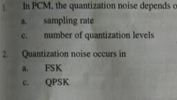
Illustration of waveforms in a PCM system., , •The error signal, (quantization noise), is inversely, proportional to the number of quantization levels used, to approximate the waveform x(t), •Companding is used to improve the SQNR (signal to, quantization noise ratio) for small amplitude x(T) signals, Couch, Digital and Analog Communication Systems, Seventh Edition, , ©2007 Pearson Education, Inc. All rights reserved. 0-13-142492-0, , Figure 3–9 Compression characteristics (first quadrant shown)., , Couch, Digital and Analog Communication Systems, Seventh Edition, , ©2007 Pearson Education, Inc. All rights reserved. 0-13-142492-0, , 11

Page 12 :
Figure 3–9 Compression characteristics (first quadrant shown)., , Couch, Digital and Analog Communication Systems, Seventh Edition, , ©2007 Pearson Education, Inc. All rights reserved. 0-13-142492-0, , Figure 3–10 Output SNR of 8-bit PCM systems with and without companding., , ⎛ V peak range ⎞, ⎡S⎤, ⎟⎟, ⎢⎣ N ⎥⎦ = 4.77 + 6.02n − 20 log⎜⎜ x, dB, rms, ⎝, ⎠, , uniform quantion, , ⎡S⎤, ⎢⎣ N ⎥⎦ = 4.77 + 6.02n − 20 log[ln (1 + μ )] μ − law companding, dB, ⎡S⎤, ⎢⎣ N ⎥⎦ = 4.77 + 6.02n − 20 log[1 + ln ( A)] A − law companding, dB, , Couch, Digital and Analog Communication Systems, Seventh Edition, , ©2007 Pearson Education, Inc. All rights reserved. 0-13-142492-0, , 12

Page 13 :
Quantization Noise,, Analog to Digital Converter-A/D, EELE445, Lecture 16, , 26, , Figure 3–7 PCM trasmission system., , q(x), , Couch, Digital and Analog Communication Systems, Seventh Edition, , ©2007 Pearson Education, Inc. All rights reserved. 0-13-142492-0, , 13

Page 14 :
Quantization, , xˆn = Q ( x ), V, , x(t), , Δ, , Δ=, , 2V, M, , =, , V, 2 n −1, , M = 2n, Q(x), -V, , Quantization – Results in a Loss of Information, x(t), , Δ=, , Δ, 2, Q(x), , −, , Δ, 2, , 2V, M, , =, , V, 2n −1, , Lost Information, After sampling, x(t)=xi, , xi ∈ R, , After Quantization:, , Q(x) = x̂, x ∈ R, , 14

Page 15 :
Quantization Noise, Quantization function:, , Define the mean square distortion:, , q( x ) = ( x − Q ( x )) 2 = ~, x2, and, Δ, x − Q( x) ≤, 2, , q2 =, , Δ, 2, , 1, q 2 dq, ∫, Δ −Δ, , Quantization, , Δ=, , 2V, M, , =, , V, 2 n −1, , 2, , M =2, Δ2, =, 12, 2, (, V), =, = Pnq the quantization noise, 3M 2, n, , where M=2n, V is ½ the A/D input range,, and n is the number of bits, , 15

Page 16 :
Quantization Noise from the expectation operator:, ~, Since X is a random variable, so are Xˆ and X, So we can define the mean squared error (distortion) as :, D = E d X , Xˆ = E ( X − Q ( X )) 2, , [(, , )] [, , ], , ~, The pdf of the error is uniformly distributed : X = X − Q ( X ), f (x~ ), 1, Δ, , −, , Δ, 2, , Δ, 2, , ⎧Δ, ⎪, f (~, x) = ⎨ 2, ⎪⎩0, ~, x, , Δ ~ Δ, ≤x≤, 2, 2, otherwise, , −, , SQNR – Signal to Quantization Noise, Ratio, , 16

Page 17 :
SQNR – Signal to Quantization Noise, Ratio, Px may be found using:, , SQNR – Signal to Quantization Noise Ratio, The distortion, or “noise”, is therefore:, , Where Px is the power of the input signal, , 17

Page 19 :
A-Law Nonuniform PCM, , a=87.56 U.S, , u-Law v.s. Linear Quantization, 8 bit, Px is signal power, Relative to full scale, , Px, , 19

Page 20 :
Pulse Code Modulation, PCM, Advantage, compared with analog systems, • b is the number of bits, • γ is (S/N)baseband, Relative to full scale, • PPM is pulse position, modulation, , 20