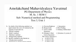
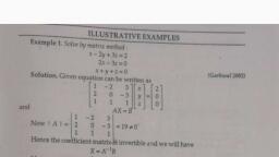
Page 1 :
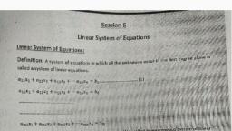
Gaussian Elimination, The purpose of this article is to describe how the solutions to a linear system are, actually found. The fundamental idea is to add multiples of one equation to the, others in order to eliminate a variable and to continue this process until only one, variable is left. Once this final variable is determined, its value is substituted back, into the other equations in order to evaluate the remaining unknowns. This method,, characterized by step‐by‐step elimination of the variables, is called Gaussian, elimination., Example 1: Solve this system:, , Multiplying the first equation by −3 and adding the result to the second equation, eliminates the variable x:, , This final equation, −5 y = −5, immediately implies y = 1. Back‐substitution of y = 1, into the original first equation, x + y = 3, yields x = 2. (Back‐substitution of y = 1 into, the original second equation, 3 x − 2 y = 4, would also yeild x = 2.) The solution of, this system is therefore (x, y) = (2, 1), as noted in Example 1., Gaussian elimination is usually carried out using matrices. This method reduces the, effort in finding the solutions by eliminating the need to explicitly write the variables, at each step. The previous example will be redone using matrices., Example 2: Solve this system:, , The first step is to write the coefficients of the unknowns in a matrix:

Page 2 :
This is called the coefficient matrix of the system. Next, the coefficient matrix is, augmented by writing the constants that appear on the right‐hand sides of the, equations as an additional column:, , This is called the augmented matrix, and each row corresponds to an equation in, the given system. The first row, r 1 = (1, 1, 3), corresponds to the first equation, 1 x +, 1 y = 3, and the second row, r 2 = (3, −2, 4), corresponds to the second equation,, 3 x − 2 y = 4. You may choose to include a vertical line—as shown above—to, separate the coefficients of the unknowns from the extra column representing the, constants., Now, the counterpart of eliminating a variable from an equation in the system is, changing one of the entries in the coefficient matrix to zero. Likewise, the counterpart, of adding a multiple of one equation to another is adding a multiple of one row to, another row. Adding −3 times the first row of the augmented matrix to the second, row yields, , The new second row translates into −5 y = −5, which means y = 1. Back‐substitution, into the first row (that is, into the equation that represents the first row) yields x = 2, and, therefore, the solution to the system: (x, y) = (2, 1)., Gaussian elimination can be summarized as follows. Given a linear system, expressed in matrix form, A x = b, first write down the corresponding augmented, matrix:, , Then, perform a sequence of elementary row operations, which are any of the, following:, Type 1. Interchange any two rows., Type 2. Multiply a row by a nonzero constant., Type 3. Add a multiple of one row to another row.

Page 3 :
The goal of these operations is to transform—or reduce—the original augmented, matrix into one of the form, where A′ is upper triangular (aij ′ = 0 for i > j), any, zero rows appear at the bottom of the matrix, and the first nonzero entry in any row, is to the right of the first nonzero entry in any higher row; such a matrix is said to be, in echelon form. The solutions of the system represented by the simpler augmented, matrix, [ A′ | b′], can be found by inspectoin of the bottom rows and back‐substitution, into the higher rows. Since elementary row operations do not change the solutions of, the system, the vectors x which satisfy the simpler system A′ x = b′ are precisely, those that satisfy the original system, A x = b., Example 3: Solve the following system using Gaussian elimination:, , The augmented matrix which represents this system is, , The first goal is to produce zeros below the first entry in the first column, which, translates into eliminating the first variable, x, from the second and third equations., The row operations which accomplish this are as follows:, , The second goal is to produce a zero below the second entry in the second column,, which translates into eliminating the second variable, y, from the third equation. One, way to accomplish this would be to add −1/5 times the second row to the third row., However, to avoid fractions, there is another option: first interchange rows two and, three. Interchanging two rows merely interchanges the equations, which clearly will, not alter the solution of the system:

Page 4 :
Now, add −5 times the second row to the third row:, , Since the coefficient matrix has been transformed into echelon form, the “forward”, part of Gaussian elimination is complete. What remains now is to use the third row to, evaluate the third unknown, then to back‐substitute into the second row to evaluate, the second unknown, and, finally, to back‐substitute into the first row to evaluate the, first unknwon., The third row of the final matrix translates into 10 z = 10, which gives z = 1., Back‐substitution of this value into the second row, which represents the, equation y − 3 z = −1, yields y = 2. Back‐substitution of both these values into the, first row, which represents the equation x − 2 y + z = 0, gives x = 3. The solution of, this system is therefore (x, y, z) = (3, 2, 1)., Example 4: Solve the following system using Gaussian elimination:, , For this system, the augmented matrix (vertical line omitted) is, , First, multiply row 1 by 1/2:, , Now, adding −1 times the first row to the second row yields zeros below the first, entry in the first column:

Page 5 :
Interchanging the second and third rows then gives the desired upper‐triangular, coefficient matrix:, , The third row now says z = 4. Back‐substituting this value into the second row, gives y = 1, and back‐substitution of both these values into the first row yields x = −2., The solution of this system is therefore (x, y, z) = (−2, 1, 4)., Gauss‐Jordan elimination. Gaussian elimination proceeds by performing, elementary row operations to produce zeros below the diagonal of the coefficient, matrix to reduce it to echelon form. (Recall that a matrix A′ = [aij ′] is in echelon form, when aij ′= 0 for i > j, any zero rows appear at the bottom of the matrix, and the first, nonzero entry in any row is to the right of the first nonzero entry in any higher row.), Once this is done, inspection of the bottom row(s) and back‐substitution into the, upper rows determine the values of the unknowns., However, it is possible to reduce (or eliminate entirely) the computations involved in, back‐substitution by performing additional row operations to transform the matrix, from echelon form to reduced echelon form. A matrix is in reduced echelon form, when, in addition to being in echelon form, each column that contians a nonzero, entry (usually made to be 1) has zeros not just below that entry but also above that, entry. Loosely speaking, Gaussian elimination works from the top down, to produce, a matrix in echelon form, whereas Gauss‐Jordan elimination continues where, Gaussian left off by then working from the bottom up to produce a matrix in reduced, echelon form. The technique will be illustrated in the following example., Example 5: The height, y, of an object thrown into the air is known to be given by a, quadratic function of t (time) of the form y = at2 + bt + c. If the object is at height y =, 23/4 at time t = 1/2, at y = 7 at time t = 1, and at y = 2 at t = 2, determine the, coefficients a, b, and c., Since t = 1/2 gives y = 23/4, , while the other two conditions, y(t = 1) = 7 and y(t = 2) = 2, give the following, equations for a, b, and c:

Page 6 :
Therefore, the goal is solve the system, , The augmented matrix for this system is reduced as follows:, , At this point, the forward part of Gaussian elimination is finished, since the coefficient, matrix has been reduced to echelon form. However, to illustrate Gauss‐Jordan, elimination, the following additional elementary row operations are performed:, , This final matrix immediately gives the solution: a = −5, b = 10, and c = 2., Example 6: Solve the following system using Gaussian elimination:, , The augmented matrix for this system is

Page 7 :
Multiples of the first row are added to the other rows to produce zeros below the first, entry in the first column:, , Next, −1 times the second row is added to the third row:, , The third row now says 0 x + 0 y + 0 z = 1, an equation that cannot be satisfied by, any values of x, y, and z. The process stops: this system has no solutions., The previous example shows how Gaussian elimination reveals an inconsistent, system. A slight alteration of that system (for example, changing the constant term, “7” in the third equation to a “6”) will illustrate a system with infinitely many solutions., Example 7: Solve the following system using Gaussian elimination:, , The same operations applied to the augment matrix of the system in Example 6 are, applied to the augmented matrix for the present system:, , Here, the third row translates into 0 x + 0 y + 0 z = 0, an equation which is satisfied, by any x, y, and z. Since this offer no constraint on the unknowns, there are not three, conditions on the unknowns, only two (represented by the two nonzero rows in the, final augmented matrix). Since there are 3 unknowns but only 2 constrants, 3 − 2 =1, of the unknowns, z say, is arbitrary; this is called a free variable. Let z = t, where t is, any real number. Back‐substitution of z = t into the second row (− y + 5 z = −6) gives

Page 8 :
Back substituting z = t and y = 6 + 5 t into the first row ( x + y − 3 z = 4), determines x:, , Therefore, every solution of the system has the form, , where t is any real number. There are infinitely many solutions, since every real, value of t gives a different particular solution. For example, choosing t = 1 gives ( x,, y, z) = (−4, 11, 1), while t = 3 gives ( x, y, z) = (4, −9, −3), and so on. Geometrically,, this system represents three planes in R 3 that intersect in a line, and (*) is a, parametric equation for this line., Example 7 provided an illustration of a system with infinitely many solutions, how this, case arises, and how the solution is written. Every linear system that possesses, infinitely many solutions must contain at least one arbitrary parameter (free, variable). Once the augmented matrix has been reduced to echelon form, the, number of free variables is equal to the total number of unknowns minus the number, of nonzero rows:, , This agrees with Theorem B above, which states that a linear system with fewer, equations than unknowns, if consistent, has infinitely many solutions. The condition, “fewer equations than unknowns” means that the number of rows in the coefficient, matrix is less than the number of unknowns. Therefore, the boxed equation above, implies that there must be at least one free variable. Since such a variable can, by, definition, take on infinitely many values, the system will have infinitely many, solutions., Example 8: Find all solutions to the system, , First, note that there are four unknwons, but only thre equations. Therefore, if the, system is consistent, it is guaranteed to have infinitely many solutions, a condition, characterized by at least one parameter in the general solution. After the, corresponding augmented matrix is constructed, Gaussian elimination yields

Page 9 :
The fact that only two nonzero rows remain in the echelon form of the augmented, matrix means that 4 − 2 = 2 of the variables are free:, , Therefore, selecting y and z as the free variables, let y = t 1 and z = t 2. The second, row of the reduced augmented matrix implies, , and the first row then gives, , Thus, the solutions of the system have the form, , where t 1 t 2 are allowed to take on any real values., Example 9: Let b = ( b 1, b 2, b 3) T and let A be the matrix, , For what values of b 1, b 2, and b 3 will the system A x = b be consistent?, The augmented matrix for the system A x = b reads, , which Gaussian eliminatin reduces as follows:

Page 10 :
The bottom row now implies that b 1 + 3 b 2 + b 3 must be zero if this system is to be, consistent. Therefore, the given system has solutins (infinitely many, in fact) only for, those column vectors b = ( b 1, b 2, b 3) T for which b 1 + 3 b 2 + b 3 = 0., Example 10: Solve the following system (compare to Example 12):, , A system such as this one, where the constant term on the right‐hand side, of every equation is 0, is called a homogeneous system. In matrix form it, reads A x = 0. Since every homogeneous system is consistent—because x = 0 is, always a solution—a homogeneous system has eithe exactly one solution, (the trivial solution, x = 0) or infiitely many. The row‐reduction of the coefficient, matrix for this system has already been performed in Example 12. It is not necessary, to explicitly augment the coefficient matrix with the column b = 0, since no, elementary row operation can affect these zeros. That is, if A′ is an echelon form, of A, then elementary row operations will transform [ A| 0] into [ A′| 0]. From the, results of Example 12,, , Since the last row again implies that z can be taken as a free variable, let z = t,, where t is any real number. Back‐substitution of z = t into the second row (− y + 5 z =, 0) gives, , and back‐substitution of z = t and y = 5 t into the first row ( x + y − 3 z = 0), determines x:, , Therefore, every solution of this system has the form ( x, y, z) = (−2 t, 5 t, t),, where t is any real number. There are infinitely many solutins, since every real value, of t gives a unique particular solution.

Page 11 :
Note carefully the differnece between the set of solutions to the system in Example, 12 and the one here. Although both had the same coefficient matrix A, the system in, Example 12 was nonhomogeneous ( A x = b, where b ≠ 0), while the one here is the, corresponding homogeneous system, A x = 0. Placing their solutions side by side,, general solution to Ax = 0: ( x, y, z) = (−2 t, 5 t, t), general solution to Ax = b: ( x, y, z) = (−2 t, 5 t, t) + (−2, 6, 0), illustrates an important fact:, Theorem C. The general solutions to a consistent nonhomogeneous lienar, system, A x = b, is equal to the general solution of the corresponding homogeneous, system, A x = 0, plus a particular solution of the nonhomogeneous system. That is,, if x = x h represents the general solution of A x = 0, then x = x h + x represents the, general solution of A x + b, where x is any particular soltion of the (consistent), nonhomogeneous system A x = b., [Technical note: Theorem C, which concerns a linear system, has a counterpart in, the theory of linear diffrential equations. Let L be a linear differential operator; then, the general solution of a solvable nonhomogeneous linear differential, equation, L(y) = d (where d ≢ 0), is equal to the general solution of the, corresponding homogeneous equation, L(y) = 0, plus a particular solution of the, nonhomogeneous equation. That is, if y = y h repreents the general solution of L(y) =, 0, then y = y h + y represents the general solution of L(y) = d, where y is any, particular solution of the (solvable) nonhomogeneous linear equation L(y) = d.], Example 11: Determine all solutions of the system, , Write down the augmented matrix and perform the following sequence of, operations:

Page 12 :
Since only 2 nonzero rows remain in this final (echelon) matrix, there are only 2, constraints, and, consequently, 4 − 2 = 2 of the unknowns— y and z say—are free, variables. Let y = t 1 and z = t 2. Back‐substitution of y = t 1 and z = t 2 into the second, row ( x − 3 y + 4 z = 1) gives, , Finally, back‐substituting x = 1 + 3 t 1 − 4 2, y = t 1,and z = t 2 into the first row (2 w −, 2 x + y = −1) determines w:, , Therefore, every solution of this system has the form, , where t 1 and t 2 are any real numbers. Another way to write the solution is as, follows:, , where t1, t2 ∈ R., Example 12: Determine the general solution of, , which is the homogeneous system corresponding to the nonhomoeneous one in, Example 11 above., Since the solution to the nonhomogeneous system in Example 11 is, , Theorem C implies that the solution of the corresponding homogeneous system, is, (where t1, t2 ∈ R), which is obtained from (*) by, simply discarding the particular soluttion, x = (1/2,1,0,0), of the nonhomogeneous, system., Example 13: Prove Theorem A: Regardless of its size or the number of unknowns, its equations contain, a linear system will have either no solutions, exactly one, solution, or infinitely many solutions.

Page 13 :
Proof. Let the given linear system be written in matrix form A x = b. The theorem, really comes down to tthis: if A x = b has more than one solution, then it actually has, infinitely many. To establish this, let x1 and x2 be two distinct solutions of A x = b. It, will now be shown that for any real value of t, the vector x1 + t(x1 − x 2) is also a, solution of A x = b; because t can take on infinitely many different values, the desired, conclusion will follow. Since A x1 = b and A x2,, , Therefore, x1 + t(x1 − x2) is indeed a solution of A x = b, and the theorem is proved., , Gauss Elimination Method, DEFINITION 2.2.10 (Forward/Gauss Elimination Method) Gaussian, elimination is a method of solving a linear system, (consisting of, equations in unknowns) by bringing the augmented matrix, , to an upper triangular form, , This elimination process is also called the forward elimination method., The following examples illustrate the Gauss elimination procedure., EXAMPLE 2.2.11 Solve the linear system by Gauss elimination method.

Page 14 :
Solution: In this case, the augmented matrix is, proceeds along the following steps., 1. Interchange, , 2. Divide the, , and, , equation by, , 3. Add, , times the, , 4. Add, , times the, , 5. Multiply the, , equation (or, , (or, , )., , )., , equation to the, , equation to the, , equation by, , The method, , (or, , equation (or, , equation (or, , )., , )., , ).

Page 15 :
The last equation gives, first equation gives, , the second equation now gives, , Finally the, , Hence the set of solutions is, , A, , UNIQUE SOLUTION., , EXAMPLE 2.2.12 Solve the linear system by Gauss elimination method., , Solution: In this case, the augmented matrix is, proceeds as follows:, 1. Add, , times the first equation to the second equation., , 2. Add, , times the first equation to the third equation., , 3. Add, , times the second equation to the third equation, , and the method, , Thus, the set of solutions is, arbitrary. In other words, the system has INFINITE NUMBER OF SOLUTIONS., , with

Page 16 :
EXAMPLE 2.2.13 Solve the linear system by Gauss elimination method., , Solution: In this case, the augmented matrix is, proceeds as follows:, 1. Add, , times the first equation to the second equation., , 2. Add, , times the first equation to the third equation., , 3. Add, , times the second equation to the third equation, , and the method, , The third equation in the last step is, , This can never hold for any value of, , Hence, the system has NO SOLUTION.