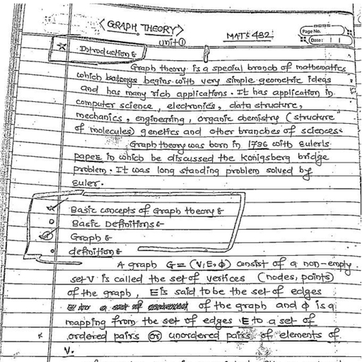
Page 1 :
ppsGniPTiVE MEASURES 2.3, , 2.1. INTRODUCTION, , Quantitative data in a mass exhibit certain general characteristics or they differ, from cach other in the following ways : ., , 1. They show a tendency to concentrate at certain values, usually somewhere in, the centre of the distribution. Measures of this tendency are called measures of, central tendency or averages., , 2. The data vary about a measure of central tendency and these measures of, deviation are called measures of variation or dispersion., , 3. The data in a frequency distribution may fall into symmetrical or, asymmetrical patterns. The measures of the direction and degree of, asymmetry are called measures of skewness., , 4. Polygons of frequency distributions exhibit flatness or peakedness of the, frequency curves. The measures of peakedness or flatness of the frequency, curves are called measures of kurtosis., , 2-2. FREQUENCY DISTRIBUTION, , When observations, discrete or continuous, are available on a single characteristic, of a large number of individuals, often it becomes necessary to condense the data as, far as possible without losing any information of interest. Let us consider the marks in, Statistics obtained by 250 candidates selected at random from among those appearing, , in a certain examination., , TABLE 2:1: MARKS IN STATISTICS OF 250 CANDIDATES, , , , , , , , , , , , 32 47 41 51 41 30 ” 18 48 53, 5d 32 31 46 15 37 32 56 2 48, 38 2% 50 40 38 42 8 2 62 5, “4 21 45 3t a7 4 44 18 7 17, 68 41 30 52 52 60 2 a8 38 ut, 41 53 48 2 28 49 42 6 41 29, 30 33 37 35 29 37 as Ww a2 qu, 43 32 24 38 as 2 dt 50 17 do, 46 50 26 15 23 42 5 52 38 46, 41 38 40 37 40 4B 45 30 28 a, 40 33 42 36 51 42 56 44 35 8, 31 51 45 41 50 53 50 32 45 48, 40 43 40 34 34 44 38 58 49 28, 40 45 19 24 34 47 37 3 37 36, 36 32 61 30 44 43 50) aL 38 45, 46 40 32 34 44 54 35 39 31 48, 48 50 43 55 43 39 41 48 53 MM, 32 31 42 34 4 32 33 4 43 w, 40 50 27 47 4 44 a4 33 47 42, 7 42 57 35 38 17 33 46 36 2, 48 50 31 58 33 44 2h » 3 a7, a7 55 57 a7 4 5d a 45 47 3, 37 52 47 46 44 50 a“ 38 42 y, 52 45 2B “a. 47 B 42 24 A, , z 40 48, , 48 44 60 38 38 M4 3~ 4B
Page 2 :
a-4, , This representation of the dat., rather confusing to mind. A better, or descending order of magnitud., reduce the bulk of the dat, , , , FUNDAMENTALS OF MATHEMATICAL STaTisti.., , ‘a does not furnish any useful information and, , way may be to express the figures in an ascendin,, €, commonly termed as array, But this docs ng, a. A much better representation is given in Table 2.2 ; ‘, , , , , , , , <a ee TABLE 22 scieceenients 7, ry here eT Mars Niele Tae, 15 i =2 0 wl |, te M =3 41 Wn =10, i " =2 42 vet Ua =13, 19 I =2 43 WH iit =8 |, al HI =2 44 vt Wt Il =12 = |, 22 I =2 45 wi |, 23 WW =3 46 WH lt =7 |, 24 Th a a7 va Ill “8 |, 25 | wi 48 wn Wat gm 4, 26 MM =3 49 Ml 23 |, 27 I =1 50 vt ual =W |, 28 tl =3 51 it = |, 29 i =2 52 wi 3, 30 wl =5 53 ul = \, 31 vat Wat =10 54 T = |, 32 WT lat =10 55 Hl =2 |, 33 ut oil =8 56 i =2, 34 woo | =11 57 I = |, 35 Mm 25 58 il s |, 36 ut =5 60 I =3 |, 37 wWhoout ol = 61 ! =1, “38 wou ow ot =17 62 | 29, 39 weit =6 68 | =1, , , , , , , , A bar (1) called tally mark is put against the number when it occurs. Having, occurred four times, the fifth occurrence is represented by putting a cross tally (1) on, the first four tallies. This technique facilitates the counting of the tally marks at the, , end., , The representation of the data as above is known as frequency distribution. Marks, are called the variable (x) and the ‘number of students’ against the marks is known as the, ‘frequency’ (f) of the variable. The word ‘frequency’ is derived from "how frequently’, variable occurs. For example, in the above case the frequency of 31 is 10 as there are, ten students getting 31 marks. This representation, though better than an ‘array’, does, not condense the data much and it is quite cumbersome to go thorough this huge, , mass of data., , If the identity of the individuals about whom a particular intormation is taken is, not relevant, nor the order in which the observations arise, then the first real step of
Page 3 :
Te,, , hy, , Noy, , nap, , ty, 8, , Min, , “ TIVE MEASURES, ypscrlP, ‘ 2:5, , condensation ie c divide the observed range of variable into a suitable numbe, ctasseinteroals anc to record the number Of observations in each class. For exam “oa is, above case, the data may be expressed as shown in Table 2-3 , —, TABL E 2-3; FREQUENCY TABLE, , the, , , , , , , jacaofstindents — |, , , , Such a table showing, the distribution of, the frequencies in the different classes is, , called a frequency fable and the manner in 20—24., , , , , , which the class frequencies are distributed 25—29 10, , over the class intervals is called the grouped ies =, , frequency distribution of the variable. 7 *, , J 40-44 54, , Remark. The classes of the type 15—19, 20—24, 4549 7, , 25—29 etc., in which both the upper and lower S54 24 ', , limits are included are called 'inchisive classes’. For i) 8, , example, the class 20— 24, includes all the values 664 5 |, , fram 20 to 24, both inclusive and the classification 65-49 I, , is termed as inclusive type classification | |, 250) |, , Fotal, , , , In spite of great importance of classification in statistical analysis, no hard and fast, rules can be laid down for it. The following points may be kept in mind for, , classification :, 1. The classes should be clearly defined and should not lead to any ambiguity., , 2. The classes should be exhaustive, ic., cach of the given values should be, included in one of the classes., , 3. The classes should be mutually exclusive and non-overlapping., , 4, The classes should be of equal width. The principle, however, cannot be rigidly, followed. If the classes are of varying width, the different class frequencies will not be, comparable. Comparable figures can be obtained by dividing the value of the, frequencies by the corresponding widths of the class intervals. The ratios thus, , obtained are called ‘frequency densities’., , 5, Indeterminate classes, ¢.¢., the open-end cl, than 'b’ should be avoided as far as possible since they create difficulty, , asses like less than ‘a ' or greater, in analysis and, , interpretation., 6. The number of clas:, preferably lie between 5 and 15. However,, , depending upon the total frequency and the d, is not less than 5 since in that case the classific, , characteristics of the population. The following formu, determine an approximate number k of classes :, , k= 143-322 logyN, where N is the total frequency. 7, The Magnitude of the Class Interval. Having fixed the number of classes, ae ae, range (the difference between the greatest and the smallest observation) » ve we, nearest integer to this value gives the magnitude of the class interval. FT ia high, intervals (i.¢., less number of classes) will yield only rough estimates Wi rable., degree of accuracy small class intervals (i.c., large number of classes) 4, , ses should neither be too large nor too small, It should, the number of classes may be more than 15, , etails required, but it is desirable that it, ation may not reveal the essential, Ja due to Struges may be used to
Page 4 :
2-6, , FUNDAMENTALS oF MATHEMATICAL 7,, - a Limits. The class limits should be, , ASS Interval and actual, Near to each other, distorted picture o, located at the, , ATISTI¢g, chosen in such a way th:, average of the observations in that cl, aS possible. If this is not the case then the clas:, f the characteristics of the data. If possible,, , at the mid-y., ‘ASS interval ar, sification give, , lun, Bas, eS a, , ee ; class limit:, , fan Points which are multiple of 0, 2, 5, 10, ... etc, so that the es be, classes are the common figures, viz., 0,2, 5, 10, ... etc., the fi ures ca Hoa is, , and simple analysis. , 8 Pable of eas,, , 2-2-1,, , Continuous Fr istributi, ble, equency Distribution. If we de, , e al with a continuo,, it is not possible to arrange the data in the class intervals of above type. Age (in years) >), , ~ Below5, Let us consider the distribution of age in years. If | 5 ormore but less than 10, class intervals are 15—19, 20—, , : 24, etc. then the persons 10 or more but less than 15, with ages between 19 and 20 years are not taken into | 15 or more but less than 20, consideration. In such a case, we form the class | 20 or more but less than 25, , , , intervals as shown in the adjoining table. and so on, 0-5, “ . . 5—ih |, Here all the persons with any fraction of age are included in one} jy_i5_ |, group or the other. For practical purposes we re-write the above 15—20, classes as shown in the adjoining table. emia, , , , The form of the frequency distribution with such classes is known as continuous, frequency distribution. It should be clearly understood that in the above classes, the, upper limits of each class are excluded from the respective classes. Such classes in, , which the upper limits are excluded from the respective classes and are included in, the immediate next class are known as ‘exclusive classes’, termed as ‘exclusive type classification’., , 2-3. GRAPHIC REPRESENTATION OF A FREQUENCY DISTRIBUTION, , It is often useful to represent a frequency distribution by means of a diagram, which makes the unwieldy data intelligible and conveys to the eye the general run of, the observations. Diagrammatic representation also facilitates the comparison of two, , or more frequency distributions. We consider below some important types of graphic, representation., , and the classification is, , 2-3-1. Histogram. In drawing the histogram of a given continuous frequency, distribution we first mark off along the x - axis all the class intervals on a suitable, scale. On each class interval erect rectangles with heights proportional to the, frequency of the corresponding class interval so that the area of the rectangle is, proportional to the frequency of the class. If, however, the classes are of unequal, width then the height of the rectangle will be proportional to the ratio of the, frequencies to the width of the classes. The diagram of continuous rectangles so, obtained is called histogram., , Remarks 1. To draw the histogram for an ungrouped frequency distribution of a variable, , | we shall have i assume that the frequency corresponding to the variate value x is spread over, the interval x-% to x+ t , Where /r is the jump from one value to the next., , | ; 2 =, | a
Page 5 :
DESCRIPTIVE MEASURES, 2-7, , 2. If the grouped frec istri, f equency distribution is i Rese}, eodtiqadisditlbutlon ane nee ae io first it is to be converted into, 3. Although th iz ; nie, Seresponding a ho. of each rectangle is proportional to the frequency of the, Pe enbivonine Hi i. t . oe of the rectangle is not proportional to the frequency, : ‘action of the class, so t i, frequency over a fraction of a class interval NER APNE Pe Gees Se Poa, , 4, The histogram of the distributi obtained as follows : istribution of marks of 250 students in Table 2-3 (page 2:5) is, , / a Pe ee frequency distribution is not continuous, we first convert it into a, continuous distribution with exclusive type classes as given in the following Table 2-4 , , , , , , , , , , , , , , , , , , , , , , , , , , , , TABI :, a Sa Ge 5 HISTOGRAM FOR FEES: DISTRIBUTION, | 14-5-19-5 9 48, 19-5-24-5 "1 aa, 245-295 10 3 =, 29-5-34:5 44 ii oe, 34-5-39-5 45 ga, 39-5445 54 £ 16, pie 37 4 ' 4 ba, 49-5-54:5 26 } |, 545-595 8 ° 0 ae on 0 "7 0 it, 595-645 5 T2428 38 3595383 B, 645-69-5 1 eT, ig. 2-1., , Note. The upper and lower class limits of the ew exclusive type classes are known as class, , boundaries., Ifd is the gap between the upper limit of any class and the lower limit of the succeeding, , class, the class boundaries for any class are then given by :, , Upper class boundary = Upper class limit + 4; Lower class boundary = Lower class limit- 5, , 23-2. Frequency Polygon. For an ungrouped distribution, the frequency, polygon is obtained by plotting points with abscissa as the variate values and the, ordinate as the corresponding frequencies and joining the plotted points by means of, straight lines. For a grouped frequency distribution, the abscissa of points are midvalues of the classintervals. For equal classintervals the frequency polygon can be, obtained by joining the middle points of the upper sides of the adjacent rectangles of, the histogram by means of straight lines. If the class intervals are of small width, the, polygon can be obtained by drawing a smooth freehand curve through the vertices of, the frequency polygon., , The frequency polygon so obtained should be extended t, at both the ends so that it meets the x-axis at the-mid-points of, classes, viz., the class before the first class and the class after th, assumed to have zero frequency., , 2-4, AVERAGES (OR MEASURES OF CENTRAL TENDENCY), , ( According to Professor Bowley, averages are "statistical cor sex, comprehend in a single effort the significance of the whole." They 51V° us, , ‘o the base line (x—axis), two hypothetical, e Jast class, each, , nstants which enable us to, dea about the