Page 1 :
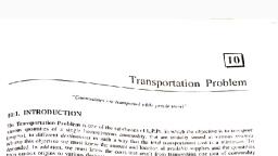
SRINIVAS UNIVERSITY, , II BBA PM/LS/HN/HA/PA/CMA, , IV SEMESTER, , UNIT III-TRANSPORTATION PROBLEMS, 3.1 INTRODUCTION, When a company have different manufacturing plants at different places, and have different places,, and have different ware houses for further distribution of products, we face problem because of, the production capacities of plants are different that it is not possible to ship all the different, requirements of ware houses from the nearest plant., When this happens, the question immediately arises as to which the most economical shipment of, product from several plants to the different ware houses. To solve such problem 'Operation, Research' helps which involves mathematical techniques called Transportation method., Examples of transportation problem:, Source, Destination, , Commodity, , Objective, , plants, , Markets, , Finished goods, , Minimizing total cost of, shipping, , plants, , Finished goods, warehouse, , Finished goods, , Minimizing total cost of, shipping, , Finished goods, warehouse, , Markets, , Finished goods, , Minimizing total cost of, shipping, , suppliers, , Plants, , Raw material, , Minimizing total cost of, shipping, , suppliers, , Raw material, warehouse, , Raw material, , Minimizing total cost of, shipping, , Raw material, warehouse, , Plants, , Raw material, , Minimizing total cost of, shipping, , The transportation problem is operational research is concerned with findings the minimum cost, of transporting a single commodity from a given number of sources (eg. Factories) to a given, number of destination (eg.warehouse). These types of problems can be solved by general network, methods, but here we use a specific transportation algorithm.

Page 2 :
SRINIVAS UNIVERSITY, , II BBA PM/LS/HN/HA/PA/CMA, , IV SEMESTER, , 3.2 ANALYSIS OF THE PROBLEM, The given problem transforms in to table form it is similar to formation of linear, Programming problem., , Schematic diagram of simple transportation problem.

Page 4 :
SRINIVAS UNIVERSITY, , II BBA PM/LS/HN/HA/PA/CMA, , •, , c i,j = unit cost of shipping from source i to destination j, , •, , x i,j = amount shipped from source i to destination j, , •, , a i = supply at source i, , •, , b j = demand at destination j, , IV SEMESTER, , Sources are represented by rows while destinations are represented by columns. In general, a, transportation problem has m rows and n columns. The problem is solvable if there are exactly, (m+n-1) basic variables., , Types of Transportation Problems, There are two different types of transportation problems based on the initial given information:, • Balanced Transportation Problems: cases where the total supply is equal to the total, demand., •, , Unbalanced Transportation Problems: cases where the total supply is not equal to the, total demand. When the supply is higher than the demand, a dummy destination is, introduced in the equation to make it equal to the supply (with shipping costs of $0); the, excess supply is assumed to go to inventory. On the other hand, when the demand is higher, than the supply, a dummy source is introduced in the equation to make it equal to the

Page 5 :
SRINIVAS UNIVERSITY, , II BBA PM/LS/HN/HA/PA/CMA, , IV SEMESTER, , demand (in these cases there is usually a penalty cost associated for not fulfilling the, demand)., In order to proceed with the solution of any given transportation problem, the first step consists in, verifying if it is balanced. If it is not, it must be balanced accordingly., The lpSolve package from R contains specific functions for solving linear programming, transportation problems. For the following example, let’s consider the following mathematical, model to be solved:

Page 6 :
SRINIVAS UNIVERSITY, , II BBA PM/LS/HN/HA/PA/CMA, , IV SEMESTER, , 3.3 METHODS OF MAKING THE INTIAL ASSIGNMENT, The first step in the transportation method as stated above, consists in making an, initial assignment in such a manner that a basic feasible solution (number of occupied cells equals, m + n - 1) is obtained various methods of making such an assignment are available., DEFINITIONS, 1. Feasible Solution: A set of non-negative individual allocations (Xij> 0) which simultaneously, removes deficiencies, is called feasible solution., 2. Basic Feasible Solution: A feasible solution to an 'm' origin and 'n' destination problem is said, to be basic if the number of positive allocations are (m + n - 1). If the number of allocations in a, basic feasible solution are less than (m + n - 1) then it is called an "Degenerate Basic Feasible, Solution., 3. Optimal Solution: A feasible is said to be optimal if it minimizes the total transportation cost., FINDING AN INTIAL BASIC FEASIBLE SOLUTION, An initial basic feasible solution to 'Transportation' problem can be found by anyone of the three, following methods., 1. North west corner rule (NWC), 2. Least cost method, 3. Vogels approximation method (VAM), , 3.4 NORTH WEST CORNER RULE:, Step 1:, Start with the cell in the upper left hand corner cell of the transportation table., Step 2 :, Allocate as many units as possible without violation the restrictions on total supply for the row, and total demands for the column., Step 3 :, Move one cell to the right if there is any remaining supply otherwise, move one cell down. If both, are impossible. Stop or got to step 2., Step 4:, An example is considered at this juncture to illustrate the application of NWC rule., If both, the demand in the column as well as to the supply in the row, are exhausted, then there is, a tie for the next allocation. An arbitrary tie breaking choice is made. Make the next allocation of, magnitude in the cell in either the column (or) the next row.

Page 7 :
SRINIVAS UNIVERSITY, , II BBA PM/LS/HN/HA/PA/CMA, , IV SEMESTER, , Step 5:, Continue the procedure until all the rim requirements., Example 1:, Origin\Destination, , D1, , D2, , D3, , D4, , O1, O2, O3, Requirement, , 6, 5, 8, 35, , 8, 1, 9, 28, , 8, 9, 7, 32, , 5, 7, 3, 25, , Origin, Capacity, 30, 40, 50, , First allocation is made in the cell O1D1. Since the origin O1has 30 units available and the, destination center D1 requires 35units. We allocate aii the 30 units from origin O1to the destination, center D1 and indicated by the encircled 30 in cell O1D1 of table 1.Now that the supply has been, exhausted we move down to second row (row O2)and allocate D1 requirement, 5 units, from the, capacity of origin O1. Thus we have met the demand at D1 completely,and so we move to right, under column D2 in second row. Allocate the requirements of D2 in the cell O2D2 from the balance, of supply from O2(35units). We continue in this way, stair-stepping down the table until all the, allocations, have been made as shown in table 1 remaining cells accommodate to given procedure., The total cost associated with this solution is obtained by multiplying the number of units shipped, to each destination centre from each origin by the appropriate shipping cost per unit. Thus the total, distribution cost for the above shipment schedule is:, =Rs(30 × 6 + 5× 5+28 × 11+7× 9+25× 7+25×13) = Rs.1,076, Note : 1 . For any cell in which no allocation is made, the corresponding Xij is zeroi.e.,no unit is, shipped to the empty cell., 2 . The cells which get allocation are called basic cells.

Page 11 :
SRINIVAS UNIVERSITY, , Origin\Destina, tion, O1, , O2, , 10, , 10, , II BBA PM/LS/HN/HA/PA/CMA, , IV SEMESTER, , D1, , D2, , D3, , D4, , D5, , Supply, , 10, , 16, , 8, , 9, , 0, , 10, , 6, , 4, , 1, , 40, , 5, , 12, , 20, , 7, , 30, , 15, , 3, , 15, , 2, , 15, , O3, , 13, , 7, , 11, , O4, , 1, , 13, , 8, , Requirement, , 20, , 15, , 30, , 5, , 5, , 3, , 25, , 10, , 25, , Initial Transportation Cost = Xij * Cij, (ITC), = 10*10+3*10+2*15+6*1515*11+5*5+5*3+25*7, =100+30+30+90+165+25+15+175, = 630, M= No. of Row, N= No. of column, No. of allocation = 8, M+N-1=4+5-1=8, Hence, the solution is Non generate., , ILLUSTRATION 2:, Origin\Destination, , D1, , D2, , D3, , D4, , Supply, , O1, , 12, , 6, , 10, , 8, , 20, , O2, O3, O4, Requirement, , 7, 3, 2, 40, , 4, 6, 8, 30, , 2, 4, 5, 10, , 1, 1, 1, 40, , 30, 40, 30

Page 12 :
SRINIVAS UNIVERSITY, , II BBA PM/LS/HN/HA/PA/CMA, , IV SEMESTER, , Solution:, Demand, Origin, O1, , 20, , D1, , D2, , D3, , D4, , Availability, , 12, , 6, , 10, , 8, , 20, , 4, , 2, , 1, , 30, , 1, , 40, , 30, , 20, , 10, , O2, , 7, , O3, , 3, , O4, , 2, , 8, , 5, , 1, , Requirement, , 40, , 30, , 10, , 40, , 20, , 6, , 10, , 4, , 10, , 30, , First allocation is made in the cell O1D1. Since the origin O1has 40 units available and the, destination center D1 requires 20units. We allocate aii the 20 units from origin O1to the destination, center D1 and indicated by the encircled 20 in cell O1D1 of table 1. Now that the supply has been, exhausted we move down to second row (row O2)and allocate D1 requirement, 20 units, from the, capacity of origin O1. Thus, we have met the demand at D1 completely, and so we move to right, under column D2 in second row. Allocate the requirements of D2 in the cell O2D2 from the balance, of supply from O2(30units). We continue in this way, stair-stepping down the table until all the, allocations, have been made as shown in the above table remaining cells accommodate to given, procedure., The total cost associated with this solution is obtained by multiplying the number of units shipped, to each destination centre from each origin by the appropriate shipping cost per unit. Thus the total, distribution cost for the above shipment schedule is:, Initial Transportation Cost = Xij * Cij, (ITC), = 20*12+20*7+10*4+20*6+10*4+10*1+30*1, =240+140+40+120+40+10+30, = 620, M= No. of Row, N= No. of column, No. of allocation = 7, M+N-1=4+4-1=7, Hence, the solution is Non generate.

Page 13 :
SRINIVAS UNIVERSITY, , II BBA PM/LS/HN/HA/PA/CMA, , IV SEMESTER, , Note : 1 . For any cell in which no allocation is made, the corresponding Xij is zeroi.e.,no unit is, shipped to the empty cell., 2 . The cells which get allocation are called basic cells., 3.5 LEAST COST METHOD (LCM), The initial basic feasible solution obtained by this method usually gives a lower, Beginning cost. Various steps of the method are as follows., Step 1 :, Determine the lowest (smallest) cost among all the rows of the transportation table, Step 2 :, Identify the row and allocate the maximum feasible quantity in the box corresponding to the, smallest cost in the row. Then eliminate (cross off) that row (column), where an allocation is made., Step 3 :, Repeat steps 1 and 2 for the reduced transportation table until all the rim requirements are satisfied., Whenever the minimum cost is not unique, make an arbitrary choice among the minimum costs., Example:, Origin, , D1, , D2, , O1, , 6, , 8, , O2, , 5, , O3, , 8, , Requirement 35, , Destination:, D3, , D4, , Supply, , 8, , 5, , 30, , 11, , 9, , 7, , 40, , 9, , 7, , 13, , 50, , 28, , 32, , 25, , 120, , Use least cost method and find out initial solution(total minimum cost), SOLUTION:, , Since the lowest costs among all the rows of the transportation table are in the cells O1 D4 and, O2D1,we allocate maximum feasible quantity of 25 units in cell O1 D4 and 35 units in O2D1 cell.

Page 14 :
SRINIVAS UNIVERSITY, , II BBA PM/LS/HN/HA/PA/CMA, , IV SEMESTER, , These two allocations satisfy the demand of columns D1 and D4 and hence are crossed off in, transportation table for the next allocation., This is given in table 1. In the reduced transportation table, the lowest cost among cell the rows is, in the cell O3D3.

Page 15 :
SRINIVAS UNIVERSITY, , II BBA PM/LS/HN/HA/PA/CMA, , IV SEMESTER, , EG. Obtain an initial feasible solution to the following TP using Matrix Minima Method., D1, , D2, , D3, , D4, , Supply, , O1, , 1, , 2, , 3, , 4, , 6, , O2, , 4, , 3, , 2, , 0, , 8, , O3, , 0, , 2, , 2, , 1, , 10, , Demand, , 4, , 6, , 8, , 6, , 24, , Solution :, Since ∑ai= ∑bj = 24, there exists a feasible solution to the TP using the steps in the least cost, method, the first allocation is made in the cell(3,1) the magnitude being x31=4. Which satisfies the, demand at the destination D1 and we delete this column from the table as it is exhausted.

Page 16 :
SRINIVAS UNIVERSITY, , II BBA PM/LS/HN/HA/PA/CMA, , IV SEMESTER, , The second allocation is made in the cell(2,4) with magnitude x24 = min (6,8)=6. Since it satisfies, the demand at the destination D4, it is deleted from the table. From the reduced table the third, allocation is made in the cell(3,3)with magnitude x33=min (8,6)=6., The next allocation is made in the cell(2,3) with magnitude x23 of min (2,2)=2. Finally the, allocation is made in the cell(1,2)with magnitude x12=min (6,6)=6. Now all the rim requirements, have been satisfied and hence, initial feasible solution is obtained., The solution is given by, x12=6, x23=2, x24=6, x31=4, x33=6, Since the total number of occupied cell=5 < m + n - 1., We get a degenerate solution., Total cost = 6 × 2 + 2 × 2 + 6 × 0 + 4 × 0 + 6 × 2, =12 + 4 +12 = Rs.28, ILLUSTRATION 3:, Determine an initial basic feasible solution for the following TP, using least cost method., DESTINATION, , Source, , D1, , D2, , D3, , D4, , D5, , TOTAL, , O1, , 10, , 16, , 8, , 9, , 0, , 10, , O2, , 3, , 2, , 6, , 4, , 1, , 40, , O3, , 13, , 7, , 11, , 5, , 12, , 20, , O4, , 1, , 13, , 8, , 3, , 7, , 30

Page 17 :
SRINIVAS UNIVERSITY, , TOTAL, , II BBA PM/LS/HN/HA/PA/CMA, , 20, , 15, , 30, , 10, , IV SEMESTER, , 25, , Solution:, DESTINATION, D1, , D2, , D3, , D4, , D5, , TOTAL, , 0, , 10, , 10, , O1, , 10, , 16, 15, , Source, , O2, , 3, , 8, , 9, , 10, , 2, , 15, , 6, , 4, , 1, , 40, , 11, , 5, , 12, , 20, , 30, , 20, , O3, , 13, , 7, , 20, , 10, , O4, , 1, , 13, , 8, , 3, , 7, , TOTAL, , 20, , 15, , 30, , 10, , 25, , ITC = Xij*Cij, = 10*0+15*2+10*6+15*1+20*11+20*1+10*3, = 375, M+N-1=5+4-1=8, No. of allocation = 8, Hence, there exists Degeneracy.

Page 18 :
SRINIVAS UNIVERSITY, , II BBA PM/LS/HN/HA/PA/CMA, , IV SEMESTER, , ILLUSTRATION 4:, Determine an initial basic feasible solution for the following TP, using least cost method., DESTINATION, D1, , D2, , D3, , D4, , D5, , TOTAL, , O1, , 9, , 6, , 1, , 2, , 3, , 10, , O2, , 6, , 7, , 10, , 14, , 2, , 30, , O3, , 8, , 13, , 20, , 18, , 11, , 20, , O4, , 4, , 12, , 5, , 17, , 1, , 20, , O5, , 3, , 7, , 6, , 19, , 21, , 25, , TOTAL, , 15, , 25, , 35, , 20, , 10, , Source, , Solution:, DESTINATION, D1, , D2, , D3, , D4, , D5, , TOTAL, , 1, , 2, , 3, , 10, , 10, , 14, , 2, , 30, , 18, , 11, , 20, , 10, , O1, , 9, , 6, 5, , 25, , O2, , 6, , 7, , Source, , 20, , O3, , 8, , 13, , 20, 10, , O4, , 4, , 10, , 12, , 15, , 5, , 17, , 1, , 20, , 25, , 10, , O5, , 3, , 7, , 6, , 19, , 21, , TOTAL, , 15, , 25, , 35, , 20, , 10, , ITC = Xij*Cij, = 10*1+25*7+5*10+20*18+10*5+10*1+15*3+10*6, = 760, M+N-1=5+5-1=9

Page 19 :
SRINIVAS UNIVERSITY, , II BBA PM/LS/HN/HA/PA/CMA, , IV SEMESTER, , No. of allocation = 8, Hence, there exists Degeneracy., , 3.6 Vogel’s Approximation Method, Transportation problem is a special kind of Linear Programming Problem (LPP) in which goods, are transported from a set of sources to a set of destinations subject to the supply and demand of, the sources and destination respectively such that the total cost of transportation is minimized. It, is also sometimes called as Hitchcock problem., Types of Transportation problems:, Balanced: When both supplies and demands are equal then the problem is said to be a balanced, transportation problem., Unbalanced: When the supply and demand are not equal then it is said to be an unbalanced, transportation problem. In this type of problem, either a dummy row or a dummy column is added, according to the requirement to make it a balanced problem. Then it can be solved similar to the, balanced problem., Example:, , Solution:, For each row find the least value and then the second least value and take the absolute difference, of these two least values and write it in the corresponding row difference as shown in the image, below. In row O1, 1 is the least value and 3 is the second least value and their absolute difference, is 2. Similarly, for row O2 and O3, the absolute differences are 3 and 1 respectively., For each column find the least value and then the second least value and take the absolute, difference of these two least values then write it in the corresponding column difference as shown

Page 20 :
SRINIVAS UNIVERSITY, , II BBA PM/LS/HN/HA/PA/CMA, , IV SEMESTER, , in the figure. In column D1, 2 is the least value and 3 is the second least value and their absolute, difference is 1. Similarly, for column D2, D3 and D3, the absolute differences are 2, 2 and 2, respectively., , These value of row difference and column difference are also called as penalty. Now select the, maximum penalty. The maximum penalty is 3 i.e. row O2. Now find the cell with the least cost in, row O2 and allocate the minimum among the supply of the respective row and the demand of the, respective column. Demand is smaller than the supply so allocate the column’s demand i.e. 250 to, the cell. Then cancel the column D1., , From the remaining cells, find out the row difference and column difference.

Page 21 :
SRINIVAS UNIVERSITY, , II BBA PM/LS/HN/HA/PA/CMA, , IV SEMESTER, , Again select the maximum penalty which is 3 corresponding to row O1. The least-cost cell in row, O1 is (O1, D2) with cost 1. Allocate the minimum among supply and demand from the respective, row and column to the cell. Cancel the row or column with zero value., , \, Now find the row difference and column difference from the remaining cells.

Page 22 :
SRINIVAS UNIVERSITY, , II BBA PM/LS/HN/HA/PA/CMA, , IV SEMESTER, , Now select the maximum penalty which is 7 corresponding to column D4. The least cost cell in, column D4 is (O3, D4) with cost 2. The demand is smaller than the supply for cell (O3, D4)., Allocate 200 to the cell and cancel the column.

Page 23 :
SRINIVAS UNIVERSITY, , II BBA PM/LS/HN/HA/PA/CMA, , IV SEMESTER, , Find the row difference and the column difference from the remaining cells., , Now the maximum penalty is 3 corresponding to the column D2. The cell with the least value in, D2 is (O3, D2). Allocate the minimum of supply and demand and cancel the column., , Now there is only one column so select the cell with the least cost and allocate the value.

Page 24 :
SRINIVAS UNIVERSITY, , II BBA PM/LS/HN/HA/PA/CMA, , IV SEMESTER, , Now there is only one cell so allocate the remaining demand or supply to the cell

Page 25 :
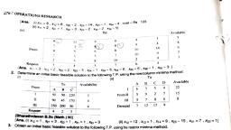
SRINIVAS UNIVERSITY, , II BBA PM/LS/HN/HA/PA/CMA, , IV SEMESTER, , No balance remains. So multiply the allocated value of the cells with their corresponding cell cost, and add all to get the final cost i.e. (300 * 1) + (250 * 2) + (50 * 3) + (250 * 3) + (200 * 2) + (150, * 5) = 2850, ILLUSTRATION 5:, Obtain IBFS to the given TP using Vogel’s approximation method., DESTINATION, , Source, , D1, , D2, , D3, , D4, , D5, , TOTAL, , O1, , 10, , 6, , 1, , 2, , 3, , 10, , O2, , 3, , 7, , 10, , 14, , 2, , 30, , O3, , 5, , 13, , 20, , 18, , 11, , 20, , O4, , 4, , 2, , 5, , 17, , 1, , 20, , O5, , 3, , 7, , 6, , 19, , 21, , 25, , TOTAL, , 15, , 25, , 35, , 20, , 10, , Solution:, , ITC= Cij*Vij, = 10*2+10*14+10*10+10*2+15*5+5*13+20*2+25*6, = 610

Page 26 :
SRINIVAS UNIVERSITY, , II BBA PM/LS/HN/HA/PA/CMA, , IV SEMESTER, , M+N-1=5+5-1=9, Since, M+N-1 solution does not match with the allocation. There exists Degeneracy., ILLUSTRATION 6:, Obtain IBFS to the given TP using Vogel’s approximation method., DESTINATION, , Source, , Solution:, , D1, , D2, , D3, , D4, , D5, , TOTAL, , O1, , 17, , 10, , 4, , 8, , 2, , 70, , O2, , 20, , 8, , 22, , 24, , 0, , 10, , O3, , 8, , 7, , 4, , 2, , 1, , 20, , O4, , 14, , 19, , 22, , 10, , 16, , 60, , TOTAL, , 25, , 30, , 15, , 50, , 40

Page 27 :
SRINIVAS UNIVERSITY, , II BBA PM/LS/HN/HA/PA/CMA, , IV SEMESTER, , ITC = 25*10+15*14+30*2+10*2+20*2+25*14+5*19+30*10, = 1155, M+N-1=5+5-1=9, Since, M+N-1 solution does match with the allocation. Therefore, the solution is Nongenerate., , UNIT III- QUESTION BANK, 1. The Transportation Problem is said to be unbalanced if, _______________., UNDERSTNADING QUESTION, A. Σai=Σbj, B. Σai≠Σbj, C. number of rows = number of columns, D. number of rows + number of columns = number of allocated cells, 2. From the following methods ___________ is a method to obtain initial solution to, Transportation Problem. KNOWLEDGE QUESTION, a) North-West, b) Simplex, c) Hungarian, d) Newton Raphson, 3. The initial solution of a transportation problem can be obtained by applying any known, method. However, the only condition is that KNOWLEDGE QUESTION, a) Rim condition should be satisfied, b) cost matrix should be square, c) one of the Xij < 0, d) None of them, 4. North – West corner refers to ____________. KNOWLEDGE QUESTION, a) top left corner, b) top right corner, c) bottom left corner, d) bottom right corner, 5. The Transportation Problem is said to be balanced if _______________. UNDERSTANDING, QUESTION, A. Σai=Σbj, B. Σai≠Σbj, C. number of rows = number of columns, D. number of rows + number of columns – 1 = number of allocated cells, 6. The occurrence of degeneracy while solving a transportation problem means that, KNOWLEDGE QUESTION, A. total supply equals total demand

Page 28 :
SRINIVAS UNIVERSITY, , II BBA PM/LS/HN/HA/PA/CMA, , IV SEMESTER, , B. the solution so obtained is not feasible, C. the few allocations become negative, D. the problem is not balanced, 7. One disadvantage of using North-West Corner Rule to find initial solution to the, transportation problem is that KNOWLEDGE QUESTION, A. it is complicated to use, B. it does not take into account cost of transportation, C. it leads to degenerate initial solution, D. all of the above, 8. The solution to a transportation problem with m-rows and n-columns is feasible if, number of positive allocations are –UNDERSTANDING QUESTION, A. m+n, B. m x n, C. m + n -1, D. all of the above, 9. If we were to use opportunity cost value for an unused cell to test optimality, it should be, KNOWLEDGE QUESTION, A. equal to zero, B. most negative number, C. most positive number, D. all of the above, 10., The allocated cells in the transportation table are called ‐‐‐‐‐‐‐‐‐‐‐‐‐ KNOWLEDGE, QUESTION, A. Occupied cells, B. Empty cells, C. Unoccupied cells, D. Both A and C, 11., A given Transportation, Problem, is said to be unbalanced, if the total supply is not equal to the total __________________, _____ KNOWLEDGE QUESTION, A. Optimization, B. Demand, C. Cost, D. Profit, 12. The purpose of the transportation approach for locational analysis is to minimize, KNOWLEDGE QUESTION, A) total costs, B) total shipping costs, C), total variable costs, D) total fixed costs

Page 29 :
SRINIVAS UNIVERSITY, , II BBA PM/LS/HN/HA/PA/CMA, , IV SEMESTER, , 13. The initial solution to a transportation problem can be generated in any manner, so long as, KNOWLEDGE QUESTION, A. it minimizes cost, B. it ignores cost, C. all supply and demand are satisfied, D. degeneracy does not exist, 14.Which of the following statements about the northwest corner rule is false? KNOWLEDGE, QUESTION, A. One must exhaust the supply for each row before moving down to the next row., B. One must exhaust the demand requirements of each column before moving to the next, column., C. When moving to a new row or column, one must select the cell with the lowest cost., D. One must check that all supply and demand constraints are met., 15. In transportation model analysis the stepping-stone method is used to KNOWLEDGE, QUESTION, A, obtain an initial optimum solution, B., obtain an initial feasible solution, C., evaluate empty cells for potential solution improvements, D., evaluate empty cells for possible degeneracy, 16. A transportation problem has a feasible solution when KNOWLEDGE QUESTION, A., all of the improvement indexes are positive, B., the number of filled cells is one less than the number of rows plus the number of, columns, C., all the squares are used, D., all demand and supply constraints are satisfied, 17. When the number of shipments in a feasible solution is less than the number of rows plus the, number of columns minus one KNOWLEDGE QUESTION, A. the solution is optimal, B. there is degeneracy, and an artificial allocation must be created, C. a dummy source must be created, D. a dummy destination must be created, 18. The stepping-stone method- UNDERSTANDING QUESTION, A., is an alternative to using the northwest corner rule, B., often involves tracing closed paths with a triangular shape, C., is used to evaluate the cost effectiveness of shipping goods via transportation, routes not currently in the solution, D., is used to identify the relevant costs in a transportation problem, 19. Which of the following methods is used for verifying the optimality of the current solution to, a transportation problem. UNDERSTANDING QUESTION, A. North West Corner Method

Page 30 :
SRINIVAS UNIVERSITY, , II BBA PM/LS/HN/HA/PA/CMA, , IV SEMESTER, , B. Least Cost Method, C. Vogel’s Approximation method, D. MODI method, 20. In a transportation problem, items are allocated from sources to destinations, UNDERSTANDING QUESTION, A. at a maximum cost, B. at a minimum cost, C. at a minimum profit, D. at a minimum revenue, 21. The linear programming model for a transportation problem has constraints for supply at each, ______, and, _______, at, each, destination., KNOWLEDGE, QUESTION, a.destination / source, b. source / destination, c. demand / source, d. source / demand, 22. The North West Corner rule KNOWLEDGE QUESTION, A. Is used to find an initial feasible solution, B. Is used to find an optimal solution, C. Is based on the concept of minimizing opportunity cost, D. None of the given, 23. If the number of allocations in the basic feasible transportation table are less than the number, of rows + number of columns -1 then the solution is said to be _________________, UNDERSTANDING QUESTION, A. non-degenrate, B. degenerate, C. optimal, D. pure assignment, 24. A initial basic feasible solution to a transportation problem can be found using, UNDERSTANDING QUESTION, A. North-West Corner Method, B. Least Cost Method, C. Vogel’s Approximation Method, D. All the above, 25. In the north west corner method, the allocation begins at UNDERSTANDING QUESTION, A. bottom left corner cell, B. Top left corner cell, C. Top Right corner cell, D. Bottom right corner cell

Page 31 :
SRINIVAS UNIVERSITY, , II BBA PM/LS/HN/HA/PA/CMA, , IV SEMESTER, , 8MARKS QUESTIONS:, 1. What do you mean by transportation problem? Explain. APPLICATION QUESTIONS, 2. Define feasible and basic feasible solution of a transportation problem. APPLICATION, QUESTION, 3. Write down the basic steps involved in solving a transportation problem using North west Corner, method. APPLICATION QUESTION, 4. Write down the basic steps involved in solving a transportation problem using Least Cost, method. APPLICATION QUESTION, 5. What do you mean by North west Corner methods? Briefly explain the procedure of North West, Corner Rule? APPLICATION QUESTION, 6. Explain the steps involved in finding an optimal solution to a transportation problem using Least, Cost Method. APPLICATION QUESTION, 7. What is Least Cost Method? Briefly explain the Procedure of formulating the Lest Cost method?, APPLICATION QUESTION, 8. Obtain the Initial Basic Feasible Solution to the following transportation problem using North, West Corner Rule., , DESTINATION, , ORIGIN, , D1, , D2, , D3, , D4, , D5, , TOTAL, , O1, , 10, , 16, , 8, , 9, , 0, , 10, , O2, , 3, , 2, , 6, , 4, , 1, , 40, , O3, , 13, , 7, , 11, , 5, , 12, , 20, , O4, , 1, , 13, , 8, , 3, , 7, , 30, , 20, , 15, , 30, , 10, , 25, , TOTAL, , 9. Find the optimal solution to the given transportation problem using Northwest corner, method., , ORIGIN, , D1, , D2, , D3, , D4, , TOTAL, , O1, , 12, , 6, , 10, , 8, , 20, , O2, , 7, , 4, , 2, , 1, , 30, , O3, , 3, , 6, , 4, , 1, , 40, , O4, , 2, , 8, , 5, , 1, , 30

Page 32 :
SRINIVAS UNIVERSITY, , II BBA PM/LS/HN/HA/PA/CMA, , TOTAL, , 40, , 30, , 10, , IV SEMESTER, , 40, , 10. Find the optimal solution to the given transportation problem using Least Cost Method., , ORIGIN, , D1, , D2, , D3, , D4, , D5, , TOTAL, , O1, , 10, , 16, , 8, , 9, , 0, , 10, , O2, , 3, , 2, , 6, , 4, , 1, , 40, , O3, , 13, , 7, , 11, , 5, , 12, , 20, , O4, , 1, , 13, , 8, , 3, , 7, , 30, , 20, , 15, , 30, , 10, , 25, , TOTAL, , 11. Obtain the Initial Basic Feasible Solution to the following transportation problem using, Least Cost Method, D1, , D2, , D3, , D4, , D5, , TOTAL, , O1, , 9, , 6, , 1, , 2, , 3, , 10, , O2, , 6, , 7, , 10, , 14, , 2, , 30, , O3, , 8, , 13, , 20, , 18, , 11, , 20, , O4, , 4, , 12, , 5, , 17, , 1, , 20, , O5, , 3, , 7, , 6, , 19, , 21, , 25, , 15, , 25, , 35, , 20, , 10, , ORIGIN, , TOTAL, , 12. Obtain the Initial Basic Feasible Solution to the following transportation problem using, Vogel’s Approximation Method., , ORIGIN, , D1, , D2, , D3, , D4, , D5, , TOTAL, , O1, , 10, , 6, , 1, , 2, , 3, , 10, , O2, , 3, , 7, , 10, , 14, , 2, , 30