Page 1 :
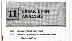
184, , , , , , , , , , 11 BREAK EVEN |, , , , , , , , ANALYSIS, , , , , , 11.1, 11.2, , 11.3, 11.4, , Concept of Break-even Point, , Variables Influencing the Break-even Point, , - Changes in Price, , - Changes in Fixed Cost, , - Changes in Variable Cost Per Unit, Business Application of Break-even Analysis, Limitations of Break-even Analysis, , Case Study, , , , , , Break-even analysis, which is also knownas cost-volume-profit analysis, is used to study the relationship between the total cost, total revenue and, total profits and losses over the whole range of output. It helps to determine, the levels of sales that is required to meet operating costs. Further, it, helps to determine the profitability or non-profitability at various levels of, sales before and after break-even points., , The break-even point for a business firm shows the volume of sales at, which the firm just breaks-even, with total revenues equal to total costs., In other words, break-even point shows the price at which the firm makes, no 4 my, , zero profits, witl, down point shows, equivalently at whic, , 1 revenues just covering costs. On the other hands the shutws the price at which revenue jist equals variable cost (or, h losses exactly equal fixed costs). In other words, the
Page 2 :
is, id, rye, , it, of, , at, cses, itor, pe, , , , Break Even Analysis 185, , break-even point comes where price is equal to average cost, while the, shut down point comes where price is equal to average variable cost., , The break-even sales level can be determined either algebraically or, graphically. The break-even sales volume can be measured by the following, formula. °, , , , Ss = F, (P - V), Where _S = _ Break-evensales in units, F = Fixed cost per period, P = Price per unit, , <, I, , Variable cost per unit, , If we multiply the sales volume in units (S) with the price per unit we will, get the sales revenue in amount., , S*=SxP, Where S* "= Break-even Sales in amount, S = Break-even Sales in Units ., P = Price per unit, , The break-even sales in amount can also be measured by dividing fixed, cost by contribution margin ratio, i.e. :, , S = F, Cc, Where S* = _ Break-evensales inamount, F =, Fixed cost per period, C = _ Contribution margin ratio, , The contribution margin ratio shows the contribution towards the recovery, , of fixed operating cost. It is the difference between price and variable cost, per unit. It is given by :, , P-V, , , , c= x 100, , The computation of break-even sales in units and amount is explained by, the following example. Let us suppose that the firm A has fixed operating
Page 3 :
186 Businéss Economics - I (BMS, BAF, BFM, BBL: SEM. | pf, , cost of 23000, the price per unit of its product is € 12 and the variable cog, per unit is % 6, Its break-even sales in units is :, , , , s- —f, P-—V, & 3,000 3000, = a, _ ., (F712 — 6) ze 500 units, , Thus, for the above firm, 500 units is break-even output. The break-even, , amount in® can be found out by multiplying the break-even output by the, Price of the output i.e. 500 x % 12 = % 6000., , The break-even amount can also be found out by the formula :, , , , , , , , Sx = F, Cc, P-—Vv :, , Where, C =, re, P- x 100 the, . june, — 12 - %6 asst, 2D x 100 wt, prof, = & x 100 = 50% furt, 12 - out, Substituting the value of C in the equation for S*, we get nar], Henx, s* = 3000 _ = 6000 . inFi;, , 50%, , It shows that the firm will start earning profit for the sales above 500 units, and the firm will have losses for the sales less than 500 units., , The firm A’s break-even point can also be explained through a break-even, chart in the following Fig. 11.1., , In the Fig. 11.1 the point B is the break-even point at which total revenue, , equals total cost. At this point the firm ceases to make loss and starts making, , profit. Thus, for sales less than f 6000 (i.e. 500 units) total revenue is less, than its operating cost and the firm incurs a loss. The absolute amount of, loss increases as the sales fall below break-even point. Conversely, for sales, greater than & 6000 (above 500 units) total revenue exceeds the operating, cost and therefore the firm starts earning profit.
Page 4 :
Break Even Analysis 187, , ¥, , , , = 9000 Total Revenue, Profit, , e TC, 5 F6000L, eV, 3, ea., % 3000, 3 Total Fixed Cost, oO, , —> xX, O 250 500 750 1000, , Output, Fig. 11.1, , The above analysis is’based on the assumption that cost and revenue, functions are linear. Thus, the total cost and total revenue lines are drawn, as straight lines and they intersect each other only at the point B. This gives, awrong impression that the whole output beyond the break-even point is, profitable. This may not be true due to changing price and cost conditions., Further, price and cost changes may not be linear, but may vary with the, output due to diminishing returns and imperfect factor and product, markets. Thus, cost and revenue functions may not be linear, but non-linear., Hence, there may be two break-even points instead of one. This is explained, inFig. 11.2., , , , , , , , , , , , Y TC, nits, ev B2, 5, yell 3, 3S, % TR, nue 3, f +? B, S$ 8 }, les Oo, it 0 a, ; 2 F ss, ale & TFC, it, —> x, oO, Qi Output Q2, , : Fig. 11.2
Page 5 :
188 Business Economics - I (BMS, BAF, BFM, BBI.: SEM.), , In the Fig. 11.2 the points B, and B, are break-even points corresponding ;,, lower and higher levels of output. For outputs lower than Q, and larg,, than Q, the firm incurs losses. For the whole range of output Q,Q, the totg, revenue exceeds total cost and therefore the firm will make profits. Th,, , shows that the firms profitable range of output lies within Q, and Q, level,, of output., , pr, , , , It can be observed from the above analysis that changes in the te, variables will influence the break-even point in different ways. This i, , explained below with the help of examples and figures., (i) Changes in Price :, , Changes in price will affect the total sales revenue and hence wil}, influence the break-even points. An increasing price will decrease a, the break-even point, while a decrease in pricé will increase int, break-even point. Let us assume that, in the example used earlierin |, the chapter, the price per unit rises to 14. Then the break-even sale, is:, , F, P-V, , wt Ot, a BOM 375 units or & 5250, , (14 - %6) 8, On the other hand, if the price falls to ¥ 10 the break-even sales is:, , = 3,000, =10 — %6, , The effect of changes in price on the break even point is explained i!, the Fig. 11:3. An increase in price will raise the total revenue curt, upwards to TR, and will bring down the break-even point to B,, whik}*, a decrease in price will shift the total revenue curve downwards? *, TR, and therefore will shift the break-even point to B,., , , , S=, , Ss = 750 units or £7500