Page 2 :
Definitions of economics, Economics is the study of how societies use scarce resources to produce valuable commodities and distribute them among different people, The branch of knowledge concerned with the production, consumption and transfer of wealth.
Page 3 :
Micro and Macro economics, Adam smith is usually considered the founder of the field of Microeconomics, the branch of economics which today is considered with the behaviour of individual entities such as markets, firms and households. In the wealth of nations (1776),Smith considered how individual pieces are set, studied the determination of prices of land, labour and capital and inquired in to the strengths and weaknesses of the market mechanisms.
Page 4 :
Macro Economics, It is concerned with the overall performance of the economy. Macroeconomics did not even exist in its modern form untill1936, when John Maynard Keynes published his revolutionary General Theory of Employment, Interest and Money., 1933 Great depression over one quarter of America’s labour force were unemployed and Keynes in this new theory developed an anlaysis of what causes business cycles with alarming spell of high unemployment and high inflation
Page 5 :
The logic of economics, Economists use the scientific approach to understand economic life. This involves observing economic affairs and drawing upon statistics and the historical record. For complex phenomena like the impact of budget deficits or the causes of inflation, historical research has provided a rich mine of insights., Often, economics relies upon analyses and theories. The theoretical approaches allow economists to make broad generalization, such as those concerning the advantages of international trade specialization or the disadvantages of tariffs and quotas.
Page 6 :
We generally distinguish two fundamentally different ways of organizing an economy. Government and markets., A market economy is one in which individuals and private firms make the major decisions about production and consumption., Extreme case of a market economy, in which the government keeps its hands off economic-decisions is called a Laissez-Faire economy., By contrast a command economy is one in which the government makes all important decision about production and distribution., No contemporary society fall completely into either of these polar categories rather all societies are mixed economies, MARKET, COMMAND AND MIXED ECONOMIES
Page 7 :
INPUTS AND OUTPUTS, Inputs are commodities or services that are used to produce goods and services. An economy uses its existing technology to combine inputs to produce out-puts, Outputs are various useful goods or services that result from the production process and are either consumed or employed in further production.
Page 8 :
FACTORS OF PRODUCTION, Land or More general resources, Labour consists of human time spent in production, Capital forms the durable goods of an economy
Page 10 :
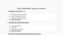
MANAGERIAL ECONOMICS, Managerial economics is a branch of economics involving the application of economic methods in the managerial decision-making process. ... Managerial economics focuses on increasing the efficiency of organizations by employing all possible business resources to increase output while decreasing unproductive activities
Page 11 :
MANAGERIAL ECONOMICS, Art and Science: Management theory requires a lot of critical and logical thinking and analytical skills to make decisions or solve problems. Many economists also find it a source of research, saying it includes applying different economic concepts, techniques and methods to solve business problems., , Micro Economics: In managerial economics, managers typically deal with the problems relevant to a single entity rather than the economy as a whole. It is therefore considered an integral part of microeconomics., , Uses Macro Economics: A corporation works in an external world, i.e. it serves the consumer, which is an important part of the economy., For this purpose, it is important that managers evaluate the various macroeconomic factors such as market dynamics, economic changes, government policies, etc., and their effect on the company., Multidisciplinary: It uses many tools and principles that belong to different disciplines, such as accounting, finance, statistics, mathematics, production, operational research, human resources, marketing, etc., Prescriptive/Normative Discipline: By introducing corrective steps it aims at achieving the objective and solves specific issues or problems., Management Oriented: This serves as an instrument in managers’ hands to deal effectively with business-related problems and uncertainties. This also allows for setting priorities, formulating policies, and taking successful decision-making., Pragmatic: The solution to day-to-day business challenges is realistic and rational.
Page 12 :
THE CONCEPT OF MANAGERIAL ECONOMICS, Liberal Managerialism, A market is a democratic space where people make their choices and decisions in a liberal way. The organization and the managers must function according to the demand of the customers and market trends; otherwise, this can lead to business failures., Normative managerialism, The managerial economics normative view states that administrative decisions are based on experiences and practices of real life. They have a systematic method for the study of demand, forecasting, cost control, product design and promotion, recruitment, etc., Radical Managership, Managers have to have a creative approach to business concerns, i.e. they have to make decisions to improve the current situation or circumstance. We concentrate more on the need and satisfaction of the consumer rather than just the maximization of income., Managerial economic values, The excellent macroeconomist N. Gregory Mankiw has given ten principles to explain the significance of business operations in managerial economics
Page 13 :
THE PRODUCTION POSSIBILITY FRONTIER, Countries cannot have unlimited amounts of all goods. They are limited by the resources and the technologies available to them. They need to choose among the limited opportunities., Examples Guns and butter. The guns of course represent the military spending and the butter stands for civilian spending
Page 14 :
PRINCIPLES OF MANAGERIAL ECONOMICS, Principles of How People Decide, Let us go through the following principles to understand how decision-making takes place in real life:, Humans face tradeoffs: To make decisions, people have to make choices on whether to choose from the different options available., Price of Opportunity: Each decision involves a cost of opportunity which is the cost of those options that we let go of while choosing the most appropriate one., Feel fair about the margin: People typically think about the margin or income they receive before investing in a specific project or individual with their money or resources., People respond to stimulus: Decisions to be made highly depend on incentives related to a product, service or activity. Negative incentives discourage people, whilst positive incentives encourage people.
Page 15 :
PRINCIPLES OF MANAGERIAL ECONOMICS, Principles of How People Interact, Communication and market impact business transactions. Let us take a look at the following related principles to justify the statement:, Trade Could Better Anyone: The theory states that trade is a way for people to share. Everyone gets an opportunity to offer those good products or services they make. And buy those products or services that other people are good at manufacturing., Markets usually represent a good way to organize economic activity, Markets often serve as a means of customer and product interaction. Consumers express their desires and expectations (demands) while producers determine whether or not to manufacture necessary products or services., Governments may often boost the performance of the market, During the time of adverse market conditions, or for the benefit of society, the government intervenes in business operations. Another such example is when the government agrees on minimum wages for the benefit of workers.
Page 16 :
PRINCIPLES OF MANAGERIAL ECONOMICS, Principles on How Economy Works, The following theory outlines the economic role of an organization’s functioning:, The standard of living of a country depends on its capacity to generate goods and services, The companies must be productive enough to produce products and services for the development of a country’s economy. Ultimately it meets the demand of the customer and enhances GDP to increase the standard of living in the country., Prices increase when the government’s printing lots of money., If surplus money is available with citizens, their capacity to spend increases, eventually leading to a rise in demand. Inflation takes place when the manufacturers are unable to satisfy market demand., Society faces a short-term correlation between unemployment and inflation, The government introduces numerous economic policies to reduce unemployment. Such policies target in the short term, to improve the economy and what kind of practice contributes to inflation.
Page 17 :
PRINCIPLES OF MANAGERIAL ECONOMICS, Scope of Managerial Economics, Managerial economics is commonly used to deal with various business problems within organizations. Both micro and macroeconomics have an equal effect on the organization and its working. The points which follow illustrate its significance:
Page 18 :
MICRO ECONOMY APPLIED TO OPERATIONAL MATERS, The various theories or principles of microeconomics used to solve the internal problems of the organization arising in the course of business operations are as follows:, Demand Theory: Demand Theory emphasizes the behavior of the consumer towards a product or service. This takes into account the customers’ desires, expectations, preferences, and conditions to enhance the manufacturing process., Decisions on Production and Production Theory: This theory is primarily concerned with the volume of production, process, capital and labor, costs involved, etc. It aims to optimize production to meet customer demand., Market Structure Pricing Theory and Analysis: It focuses on assessing a product’s price taking into account the competition, market dynamics, production costs, optimizing sales volume, etc., exam and management of profit: the companies are operating for assets hence they always aim to maximize profit. It also depends on demand from the market, input costs, level of competition, etc., Decisions on capital and investment theory: Capital is the most important business element. This philosophy takes priority over the proper distribution of the resources of the company and investments in productive programs or initiatives to boost operational performance.
Page 19 :
MACRO ECONOMICS, Macro-Economics Applied to Business Environment, Any organization is greatly affected by the environment in which it operates. The business climate can be defined as:, Economic environment: A country’s economic conditions, GDP, government policies, etc. have an indirect effect on the company and its operations., Social environment: The society in which the organization, like employment conditions, trade unions, consumer cooperatives, etc., functions also affects it., Political environment: a country’s political system, whether authoritarian or democratic; political stability; and attitude towards the private sector, impact the growth and development of the organization., Management economics is an important method for assessing the company’s priorities and objectives, the organization’s current role, and what the management can do to fill the void between the two.
Page 20 :
SLOPE OR GRADIANT, In mathematics, the slope or gradient of a line is a number that describes both the direction and the steepness of the line, Slope is often denoted by the letter m; there is no clear answer to the question why the letter m is used for slope, but its earliest use in English appears in O Brian (1844) who wrote the equation of a straight line as "y = mx + b" and it can also be found in Todhunter(1888) who wrote it as "y = mx + c".
Page 21 :
VERTICAL CHANGE TO THE HORIZONTAL CHANGE, Slope is calculated by finding the ratio of the "vertical change" to the "horizontal change" between (any) two distinct points on a line. Sometimes the ratio is expressed as a quotient ("rise over run"), giving the same number for every two distinct points on the same line. A line that is decreasing has a negative "rise". The line may be practical - as set by a road surveyor, or in a diagram that models a road or a roof either as a description or as a plan.
Page 22 :
MEANING OF m, The steepness, incline, or grade of a line is measured by the absolute value of the slope. A slope with a greater absolute value indicates a steeper line. The direction of a line is either increasing, decreasing, horizontal or vertical., A line is increasing if it goes up from left to right. The slope is positive, i.e. { m>0}., A line is decreasing if it goes down from left to right. The slope is negative, i.e. { m<0}., If a line is horizontal the slope is zero. This is a Constant function., If a line is vertical the slope is undefined
Page 23 :
DEMAND AND SUPPLY EQUILIBRIUM
Page 24 :
Slope m= ∆X/∆Y= tan(θ)
Page 25 :
Change of a change of a change, The rise of a road between two points is the difference between the altitude of the road at those two points, say y1 and y2, or in other words, the rise is (y2 − y1) = Δy. For relatively short distances, where the earth's curvature may be neglected, the run is the difference in distance from a fixed point measured along a level, horizontal line, or in other words, the run is (x2 − x1) = Δx. Here the slope of the road between the two points is simply described as the ratio of the altitude change to the horizontal distance between any two points on the line., In mathematical language, the slope m of the line is, { m={ {y2-y1}/{x{2}-x{1}}.The concept of slope applies directly to grades or gradients in geography and civil engineering Through trignometry, the slope m of a line is related to its angle of incline θ by the tangent function {m=tan(theta )}Thus, a 45° rising line has a slope of +1 and a 45° falling line has a slope of −1.
Page 26 :
What is a market?, A market is a mechanism through which buyers and sellers interact to determine prices and exchange of goods and services, Market Equilibrium: A market equilibrium represents a balance among all the different buyers and sellers.
Page 27 :
THEORY OF SUPPLY AND DEMAND, The increase in the price of fuel has occurred either because the demand for the fuel has increased or because the supply of the fuel has decreased. The same is true for every market, changes in supply and demand drive changes in output and prices., If you understand how demand and supply work, then you have understood the market economy.
Page 28 :
THE DEMAND CURVE, Law of downward sloping demand: When the price of a commodity is raised (and other things are held constant), buyers tend to buy less of the commodity. Similarly when the price is lowered, other things being constant, quantity demand increases
Page 29 :
THE SUPPLY CURVE, The supply schedule ( or supply curve) for a commodity shows the relationship between its market price and the amount of that commodity that producers are willing to produce and sell, other things held constant., The upward sloping supply curve for an individual commodity. One important reason for the upward slope is the law of diminishing returns.
Page 30 :
EQUILIBRIUM WITH SUPPLY AND DEMAND CURVE, The equilibrium price and quantity come where the amount willing supplied equals the amount willingly demanded. In a competitive market this equilibrium is found at the intersection of the supply and demand curves. There are no shortages or surpluses at the equilibrium prices
Page 31 :
KEYNES THEORY OF EMPLOYMENT, EMPLOYMENT AND OUTPUT
Page 32 :
CONSUMPTION DEMAND
Page 33 :
INVESTMENT DEMAND
Page 34 :
RATE OF INTEREST
Page 35 :
MARGINAL EFFICIENCY OF CAPITAL
Page 36 :
Factors involved in Forecasting, A firm considers various factors while forecasting such as changes in income, consumer’s taste preference, technology changes and competitive strategies while forecasting demand for its products., Demand forecasting helps organizations to plan its production, sales, recruitment and also clear old stocks accordingly. It saves money effort and prevent wastage
Page 37 :
Techniques of forecasting, Demand forecasting allows manufacturing companies to gain insight into what their consumer needs through a variety of forecasting methods. These methods include: predictive analysis, conjoint analysis, client intent surveys, and the Delphi Method of forecasting
Page 38 :
PREDICTIVE ANALYSIS/ ANALYTICS, Predictive analytics is a branch of advanced analytics that makes predictions about future outcomes using historical data combined with statistical modeling, data mining techniques and machine learning. Companies employ predictive analytics to find patterns in this data to identify risks and opportunities
Page 39 :
CONJOINT ANALYSIS, Conjoint analysis is the optimal market research approach for measuring the value that consumers place on features of a product or service. This commonly used approach combines real-life scenarios and statistical techniques with the modeling of actual market decisions, Ranking for each vector and analyzing the future requirements is a process of CONJOINT ANALYSIS given by Pro. Paul. E. Green
Page 40 :
DELPHI METHOD, The Delphi method is a forecasting process framework based on the results of multiple rounds of questionnaires sent to a panel of experts. ... This process combines the benefits of expert analysis with elements of the wisdom of crowds., Experience of seniors in the field helps us to forecast future sales and know the demand in the market
Page 41 :
TECHNIQUES IN DEMAND FORECASTING, There are three basic types—qualitative techniques, time series analysis and projection, and causal models., Time Series: A time series is a collection of observations of well-defined data items obtained through repeated measurements over time. For example, measuring the value of retail sales each month of the year would comprise a time series
Page 42 :
PROJECTION AND CAUSAL MODELS, Causal forecasting is the technique that assumes that the variable to be forecast has a cause-effect relationship with one or more other independent variables. Causal techniques usually take into consideration all possible factors that can impact the dependent variable.
Page 43 :
PURPOSE OF FORECASTING, Forecasting is a technique that uses historical data as inputs to make informed estimates that are predictive in determining the direction of future trends. Businesses utilize forecasting to determine how to allocate their budgets or plan for anticipated expenses for an upcoming period of time.
Page 44 :
AVERAGES, MOVING AVERAGES, Total of days(period)/ Number of days, EXPONENTIAL MOVING AVERAGES, EMA = Closing price x multiplier + EMA (previous day) x (1-multiplier), WEIGHTED MOVING AVERAGESDescription. A Weighted Moving Average puts more weight on recent data and less on past data. This is done by multiplying each bar's price by a weighting factor. Because of its unique calculation, WMA will follow prices more closely than a corresponding Simple Moving Average.
Page 45 :
COST ANALYSIS : PRODUCTION FUNCTION, Cost Analysis. A production function tells us how much output a firm can produce with its existing plant and equipment. The level of output depends on prices and costs. The most desirable rate of output is the one that maximizes total profit that is the difference between total revenue and total cost.
Page 46 :
PRODUCTION AND COST, Production and Costs. We've explained that a firm's total costs depend on the quantities of inputs the firm uses to produce its output and the cost of those inputs to the firm. The firm's production function tells us how much output the firm will produce with given amounts of inputs
Page 47 :
PRODUCTION ANALYSIS, PRODUCTION ANALYSIS Production Function •The technological physical relationship between inputs and outputs per unit of time, is referred to as production function. • The relationship between the inputs to the production process and the resulting output is described by a production function.
Page 48 :
COST SUMMARY, 1. The act of breaking down a cost summary into its constituents and studying and reporting on each factor. 2 : the comparison of costs (as of standard with actual or for a given period with another) for the purpose of disclosing and reporting on conditions subject to improvement.
Page 49 :
PURPOSE OF COST ANALYSIS, A cost-benefit analysis is the process of comparing the projected or estimated costs and benefits (or opportunities) associated with a project decision to determine whether it makes sense from a business perspective
Page 50 :
4 TYPES OF COST, Direct, indirect, fixed, and variable are the 4 main kinds of cost. In addition to this, you might also want to look into operating costs, opportunity costs, sunk costs, and controllable costs.
Page 51 :
DIRECT AND INDIRECT COST, A direct cost is a price that can be directly tied to the production of specific goods or services. A direct cost can be traced to the cost object, which can be a service, product, or department. Direct and indirect costs are the two major types of expenses or costs that companies can incur. Direct costs are often variable costs, meaning they fluctuate with production levels such as inventory. However, some costs, such as indirect costs are more difficult to assign to a specific product. Examples of indirect costs include depreciation and administrative expenses.
Page 52 :
FIXED AND VARIABLE COST, Businesses incur two main types of costs when they produce their goods—variable and fixed costs. Variable costs are any expenses that change based on how much a company produces and sells. ... Fixed costs, on the other hand, are any expenses that remain the same no matter how much a company produces.
Page 53 :
OPERATING COST, Operating costs are associated with the maintenance and administration of a business on a day-to-day basis. Operating costs include direct cost of goods sold (COGS) and other operating expenses—often called selling, general and administrative (SG&A)—which include rent, payroll, and other overhead costs, as well as raw materials and maintenance expenses. Operating costs exclude non-operating expenses related to financing, such as interest, investments, or foreign currency translation., The operating cost is deducted from revenue to arrive at operating income and is reflected on a company’s income statement.
Page 54 :
OPPORTUNITY COST, The opportunity cost is time spent studying and that money to spend on something else. A farmer chooses to plant wheat; the opportunity cost is planting a different crop, or an alternate use of the resources (land and farm equipment). A commuter takes the train to work instead of driving
Page 55 :
SUNK COST, sunk cost, in economics and finance, a cost that has already been incurred and that cannot be recovered. In economic decision making, sunk costs are treated as bygone and are not taken into consideration when deciding whether to continue an investment project., A manufacturing firm, for example, may have a number of sunk costs, such as the cost of machinery, equipment, and the lease expense on the factory.
Page 56 :
SUNK COST FORMULA, Sunk cost formula:, Subtract the current value from the as-new price to find the sunk cost. To calculate the sunk cost of a project, list all equipment and/or tools that can't be sold or reused. Find the purchase price and its current value to identify depreciation. Then assign a sunk cost
Page 57 :
OPPOSITE OF SUNK COST, The opposite of a sunk cost is a prospective cost, which is a sum of money due depending on future business or economic decisions. For instance, a successful business may take on prospective costs only if its decision-makers decide to expand, such as by building a new plant
Page 58 :
CONTROLLABLE COST, Controllable costs are those over which the company has full authority. Such expenses include marketing budgets and labor costs. By contrast, non-controllable costs are those that a company cannot change, such as rent and insurance. It is important for management to know the differences between these two cost types.
Page 59 :
LEAST COST COMBINATION OF INPUTS, The cost line or budget line for production is called the isocost line. The first order conditions state that the variable factors are combined in an optimal manner when the ratio of marginal products is equal to the ratio of factor prices. This optimal combination is called the least cost combination of inputs.
Page 60 :
MARGINAL PRODUCT, Marginal product or marginal physical productivity of an input (factor of production) is the change in the output resulting from employing one or more unit of a particular input ( for instance the change in the output when a firm’s labour is increased from five to six units) assuming that the quantities of other outputs are kept constant, MP= ∆Y/ ∆X
Page 62 :
ISOCOST LINE, An isocost line is a curve which shows various combinations of inputs that cost the same total amount . For the two production inputs labour and capital, with fixed unit costs of the inputs, the isocost curve is a straight line . ... The line connecting these two points is the isocost line.
Page 63 :
ISOCOST LINE CALCULATION, The isocost line is a firm's budget constraint when buying factors of production. To calculate the isocost line for a firm, begin with the total cost equation, TC = (W x L) + (r x K) and solve for K. W= wages, L =labor, r = the rent (what you pay for the use of capital), and K = capital
Page 64 :
COST MINIMIZATION
Page 65 :
FACTOR PRODUCTIVITIES AND RETURNS TO SCALE, Returns to scale measures the change in productivity after increasing all inputs of production in the long run. Under the law of diminishing marginal returns, removing inputs to a point can result in cost savings without diminishing production.
Page 66 :
FACTOR PRODUCTIVITIES AND RETURNS TO SCALE, An increasing returns to scale occurs when the output increases by a larger proportion than the increase in inputs during the production process. For example, if input is increased by 3 times, but output increases by 3.75 times, then the firm or economy has experienced an increasing returns to scale.
Page 67 :
FACTOR PRODUCTIVITIES AND RETURNS TO SCALE, This is because the total economic productivity of a country is determined by three factors (Li and Mérette, 2005) contributing to total economic production (as measured by gross domestic product [GDP]): (1) natural resources and capital input, (2) human resources or labor input, and (3) the technological base (total .
Page 68 :
FACTOR PRODUCTIVITIES AND RETURNS TO SCALE, Total factor productivity (TFP) refers to the productivity of all inputs taken together. TFP is a measure of the output of an industry or economy relative to the size of all of its primary factor inputs.
Page 69 :
FACTOR PRODUCTIVITIES AND RETURNS TO SCALE, In the monetary intertemporal model, an increase in current total factor productivity increases output, decreases the real interest rate, decreases the price level, and increases the real wage. ... The increase in output is smaller than it would be otherwise, and output may even decline.
Page 70 :
Economies of Scale vs Returns to Scale, Returns to scale refers to changes in the levels of output as inputs change, and economies of scale refers to changes in the costs per units as the number of units are increased.
Page 71 :
ECONOMIES OF SCALE, Economies of scale refers to the feature of many production processes in which the per-unit cost of producing a product falls as the scale of production rises. Increasing returns to scale refers to the feature of many production processes in which productivity per unit of labor rises as the scale of production rises
Page 73 :
DISECONOMIES OF SCALE, Diseconomies of scale happen when a company or business grows so large that the costs per unit increase. ... With this principle, rather than experiencing continued decreasing costs and increasing output, a firm sees an increase in costs when output is increased.
Page 74 :
MARGINAL USES OF PRODUCTION FUNCTION, The managerial use of the production function may be summarized as follows: It may be used to compute the least-cost combination of inputs for a given output. It may be used by the manager to obtain the most appropriate combination of input. ... Production functions help the managers in taking long-run decisions.
Page 75 :
MARGINAL USES OF PRODUCTION FUNCTION, To determine the optimum quantity of output to be produced and supplied. , To determine in advance the cost of business operations, To address alocative efficiency in the use of factor inputs in production and the resulting distribution of income to those factors, while abstracting away from the technological problems of achieving technical efficiency, as an engineer or professional manager might ...
Page 76 :
COST -AVERAGE, Average cost: Total cost (refer to cost, total) divided by the number of units produced, This refers to the cost involved per unit, Essential for all manufacturing companies, Can be calculated for service industry too, Average cost can be brought down by increasing the productivity
Page 77 :
COST- VARIABLE, A cost that varies with the level of output, such as raw material, labour and fuel costs. Variable costs equal total cost minus fixed cost
Page 78 :
COST-PUSH INFLATION, Inflation originating on the supply side of markets from a sharp increase in costs. In the aggregate supply and demand framework, cost push is illustrated as an upward shift of the curve. Also called as supply shock inflation.
Page 79 :
COST MARGINAL, The extra cost (or the increase in total cost) required to produce 1 extra unit of output (or the reduction in total cost from producing 1 unit less)
Page 80 :
COST FIXED, The cost a firm would incur even if its output for the period in question was zero. Total fixed cost is made up of such individual contractual costs as interest, payments, mortgage payments, and directors’ fees. Or just salaries to the security team
Page 81 :
COST MINIMUM, The lowest attainable cost per unit (whether average, variable or marginal). Every point on an average cost curve is a minimum in the sense that it is the best the firm can do with respect to cost for the output which that point represents. Minimum average cost is the lowest point or points on the curve.
Page 82 :
THE LINK BETWEEN PRODUCTION AND COSTS, The price inputs like labour are important factors influencing costs. Higher rents and wages mean higher costs. The relationship between cost and production helps us explain why average cost curves tend to be U shaped.
Page 83 :
Factors for cost, Fuel, transportation cost, Technology cost, Taxation cost, Labour laws, Rent and land agreement costs, Inflation in a given country, Least cost rule: To produce a given level of output at least cost, a firm should buy inputs until it has equalized the marginal product per rupee spent on each input this implies that= Marginal product of L/ Price of L
Page 84 :
Factors markets: Labour, land and capital, Questions about the distribution of income are among the most controversial in all economics. Some people argue that high incomes are the unfair result of past inheritance and luck while poverty stems from discrimination and lack of opportunity. Others believe that people get what they deserve and that interfering with the market distribution of income would injure an economy’s efficiency and make every one worse off.
Page 85 :
INCOME, In measuring the economic status of a person or a nation, the two yardsticks most often used are income and wealth. Income refers to the flow of wages, interest payments, dividends and other things of value accruing during a period of time (usually a year). The aggregate of all incomes is national income, the components are: Labour income(wages and salaries),benefits and other labour income. Property income: proprietors income, rental income, corporate profits, net interest. The biggest share of national income goes to labour, either as wages or salaries or as fringe benefits. The remainder goes to the different types of property income: rent, net interest, corporate profits and proprietors income. The last category basically includes the returns to the owners of small business.
Page 86 :
Earnings of Market economy, The earnings in a market economy are distributed to the owners of the economy’s factors of production in the form of wages, profits, rent and interest.
Page 87 :
FACTOR INCOME VS PERSONAL INCOMES, It is important to understand the distinction between factor incomes and personal incomes. The factor incomes are the division between labour and property incomes. But the same person may own many different factors of production. For example, someone might receive a salary, earn interest on money in a savings account, get dividends from share in a mutual fund and collect rent on a real estate investment. In economic language we observe that a person’s market income is simply the quantities of factors of production sold by that person times the wages or price of each factor.
Page 88 :
FACTOR INCOME VS PERSONAL INCOME, Almost three quarters of national income goes to labour while the rest is distributed as some of ruturns to capital. The last quarter century has been a turbulent one. What has been the impact of oil price shocks, the computer revolution, globalization, corporate downsizing and the long economic boom on labor’s share of the total income pie?
Page 89 :
WEALTH, We see that some incomes comes from interest or dividends on holding of bonds or stocks. This brings us to the second important economic concept wealth: Wealth consists of the net rupee value of assets owned at a given point in time. Note that wealth is a stock (like the volume of a lake) while income is a flow per unit in time ( like the flow of a stream). A household’s wealth includes its tangible items( house car and other consumer durable goods and land) and its financial holdings such as (cash, savings account, bonds and stocks) all items that are of value are called assets while those that are owed are called liabilities. The difference between total assets and total liabilities is called wealth or net worth.
Page 90 :
THE LABOUR MARKET, How wages are set in a market economy. The supply of labour and the determination of wages under competitive conditions. The general wage level: in analyzing labour earnings, economists tend to look at the average real wage, which represents the purchasing power of an hour’s work or the money wages divided by the cost of living
Page 91 :
DEMAND FOR LABOUR, MARGINAL PRODUCTIVITY DIFFERENCE: there exists a relationship between the quantity of labour inputs and amount of output. By the law of diminishing returns each additional unit of labour input will add a smaller and smaller slab of out put. To begin with, the marginal productivity of labour will rise if workers have more or better capital goods to work with. Compare: Bulldozer vs. hand showel, horse travel vs aeroplanes, educated vs uneducated, highly skilled vs no skill,
Page 92 :
COMPARISONS, Light bulbs replace oil lamps, airplanes replace horses, xerography replace quill and ink, computers replace abacuses and internet commerce invade traditional ways of doing business. Hence the productivity of an average Indian has increased compared to 1900.
Page 93 :
AMERICA VS MEXICO, Additionally when compared to the united states, a country like Mexico has much less capital to work with: many of the roads are unpaved, few computers and fax machines are in use, and much of the equipment is old and poorly maintained. All these factors make labour’s marginal productivity low and tend to reduce wages
Page 94 :
THE SUPPLY OF LABOUR, Labour supply refers to the number of hours that the population desires to work in gainful activities. The three key elements for labour supply are hours per worker, labour force participation and immigration., The substitution effect and the income effect: with higher wages you want to buy more goods and services and in addition you will want more leisure time. You can afford to take longer vacations or to retire either than you otherwise would.
Page 95 :
The supply of labour, Put yourself in the shoes of a worker who has just been offered higher hourly rates and is free to choose the number of hours to be worked. You are tugged in two different directions. On one side is the substitution effect, because each hour of work is now better paid, each hour of leisure has become more expensive, you thus have an incentive to substitute extra work for leisure.
Page 96 :
LABOUR FORCE PARTICIPATION, Women and migration: One of the most dramatic developments in recent decades has been the sharp influx of women into the workforce. The labour force particiapation rate of women., Immigration both legal and illegal plays a role in the supply of labour force
Page 97 :
Labour laws and unions, Differential wages, Labour unions, Min and Max wage, High skilled job, Low skilled jobs, Economic discrimination against women
Page 98 :
LAND AND CAPTIAL, In a capitalistic economy a country’s capital and other assets are privately owned. Similarly in a mixed economy like ours, we find that the assets are owned by both government organizations as well as private entities., Land and rent: Land is an essential factor of production for any business. The unusual feature of land is that its quantity is fixed and completely unresponsive to price, The price of using land or other inputs in fixed supply is called its rent (or pure economic rent)., Rent ( or pure economic rent) is the payment for the use of factors of production that are fixed in supply., Because the supply of land is inelastic, land will always work for whatever it can earn. Thus the value of the land derives entirely from the value of the product, and not vice versa.
Page 99 :
CAPITAL AND INTEREST, Economic analysis traditionally divides factors of production in to three categories: land, labour and capital. The first two of these are called primary or original factors of production, whose supplies are determined largely outside the market place. To them we add a produced factor of production, capital.
Page 100 :
CAPITAL AND INTEREST, Capital (or capital goods) consists of those durable produced good that are in turn used as productive inputs for further production. Some capital goods might last a few years. While others might last for a century or more. But the essential property of a capital good is that it is both an input and an output., There are three major categories of capital goods: structure (such as factories and home), equipment (consumer durable goods like automobiles and producer durable equipment like machine tools and computers and inventories of inputs and outputs (such as cars in dealers’ lots)
Page 101 :
FEW DEFINITIONS, Capital goods: durable produced goods used for further production, Rentals: net annual dollar/ rupee returns on capital goods, Rate of return on capital: net annual receipts on capital divided by dollar/ rupee value of capital (measure as percent per year), Interest rate: yield on funds, measured as percent per year, Real interest rate: yield on funds corrected for inflation, also measured as percent per year, Present value: value today of a stream of future returns generated by an asset., Profits: a residual income item equal to revenues minus costs.
Page 102 :
LAND AND RENT, Assets generate streams of income in future periods. By calculating the present value, we can convert the stream of returns in to a single value today. This is done by asking what amount of dollar/ rupee today will generate the stream of future returns when invested at the market interest rate.
Page 103 :
IMPORTANT QUALIFICATIONS OF CLASSICAL CAPITAL THEORY INCLUDE THE FOLLOWING:, Technological change shifts the productivity of capital; imperfect foresight means the capital’s return is highly volatile and investors must consider the impact of taxes and inflation.
Page 104 :
PROFITS ARE REVENUES LESS COST, Profits are revenues less cost. Reported business profits are chiefly corporate earnings. Economically, we distinguish three categories of profits.(a) an important source of profits is implicit returns. Firms generally own many of their own nonlabour factors of production- capital, natural resources and patents. In these cases the implicit retruns on unpaid or owned inputs is part of profits. (b) another source of profits is uninsurable risk, particularly that associated with the business cycle or sovereign risk. © finally innovational profits will be earned by entrepreneurs who introduce new product or innovation
Page 105 :
TYPES OF COMPETITION, Economists have identified four types of competition—perfect competition, monopolistic competition, oligopoly, monopoly and Monopsony
Page 106 :
PERFECT COMPETITION, In economic theory, perfect competition occurs when all companies sell identical products, market share does not influence price, companies are able to enter or exit without barrier, buyers have perfect or full information, and companies cannot determine prices.
Page 107 :
MONOPOLISTIC COMPETITION, Monopolistic competition characterizes an industry in which many firms offer products or services that are similar (but not perfect) substitutes. Barriers to entry and exit in a monopolistic competitive industry are low, and the decisions of any one firm do not directly affect those of its competitors.
Page 108 :
OLIGOPOLY MARKET STRUCTURE, Oligo- in Greek means few, Poly means to sell, A market structure in which a market or industry is dominated by a small number of large sellers or producers
Page 109 :
MONOPOLY, A monopoly is as described by Irving Fisher, a market with the "absence of competition", creating a situation where a specific person or enterprise is the only supplier of a particular thing.
Page 110 :
MONOPSONY, In economics, a monopsony is a market structure in which a single buyer substantially controls the market as the major purchaser of goods and services offered by many would-be sellers
Page 117 :
PERFECT COMPETITION, In economics, specifically general equilibrium theory, a perfect market, also known as an atomistic market, is defined by several idealizing conditions, collectively called perfect competition, or atomistic competition. , A perfect competition is one in which the number of buyers and sellers is very large, all engaged in buying and selling a homogeneous product with out any artificial restrictions and possessing perfect knowledge of market at a time
Page 118 :
PERFECT COMPETITION
Page 120 :
AR= AVERAGE REVENUE,MR= MARGINAL REVENUE= PRICE AND D-DEMAND LINE
Page 122 :
THREE EXAMPLES OF PERFECT COMPETITION, Agriculture: In this market, products are very similar. Carrots, potatoes, and grain are all generic, with many farmers producing them. ..., Foreign Exchange Markets: In this market, traders exchange currencies. ..., Online shopping: We may not see the internet as a distinct market.
Page 123 :
PRODUCT MARKET MODELS
Page 127 :
MONOPOLISTIC COMPETITION, Essentially a monopolistic competitive market is one with freedom of entry and exit, but firms can differentiate their products. ... Therefore, they have an inelastic demand curve and so they can set prices
Page 128 :
MONOPOLISTIC COMPETITION, Monopolistic competition is a type of imperfect competition such that many producers sell products that are differentiated from one another as goods but not perfect substitutes (such as from branding, quality, or location). In monopolistic competition, a firm takes the prices charged by its rivals as given and ignores the impact of its own prices on the prices of other firms., Unlike in perfect competition, firms that are monopolistically competitive maintain spare capacity. Models of monopolistic competition are often used to model industries. Textbook examples of industries with market structures similar to monopolistic competition include restaurants, cereal, clothing, shoes, and service industries in large cities.
Page 129 :
MONOPOLISTIC COMPETITION
Page 130 :
MONOPOLISTIC COMPETITION
Page 131 :
MONOPOLISTIC COMPETITION VS MONOPOLY, Monopolistic competition is different from a monopoly. A monopoly exists when a person or entity is the exclusive supplier of a good or service in a market. The demand is inelastic and the market is inefficient.
Page 132 :
Elasticity VS Inelasticity of Demand, Inelasticity and elasticity of demand refer to the degree to which demand responds to a change in another economic factor, such as price, income level, or substitute availability. Elasticity measures how demand shifts when other economic factors change. When fluctuating demand is unrelated to an economic factor, it is called inelasticity., Price is the most common economic factor used when determining elasticity or inelasticity. Other factors include income level and substitute availability.
Page 133 :
ELASTIC DEMAND, Elastic demand means there is a substantial change in quantity demanded when another economic factor changes (typically the price of the good or service), whereas inelastic demand means that there is only a slight (or no change) in quantity demanded of the good or service when another economic factor is changed., The elasticity of demand is an important economic concept. This article will explore more about the concepts of elasticity and demand, and the difference between demand that is elastic and demand that is considered inelastic.
Page 134 :
CHAPTER 02, Demand Analysis
Page 135 :
INTRODUCTION, The word 'demand' is so common and familiar with every one of us that it seems not required to define it. , But Some time the word demand create confusion in the minds of people because it is sometimes confused with other words such as Desire, Wish, Want, Etc., Demand in economics means a desire to own a product or goods supported by willingness and ability to pay for it., If you have a desire to buy a certain commodity, say a car, but you do not have the adequate means to pay for it, it will simply be a wish, a desire or a want and not demand., Demand= Desire To Own + Willingness To Pay + Ability To Pay
Page 136 :
Companies must measure not only how many people want their product, but also how many are willing and have the ability to buy it.
Page 139 :
TYPES OF DEMAND, Price Demand: Price Demand is a demand for different quantities of a product or service that consumers intend to purchase at a given price assuming other factors, such as prices of the related goods, level of income of consumers, and consumer preferences, remain unchanged. Price demand is inversely proportional to the price of a product or service. As the price of a product or service rises, its demand falls and vice versa. Price demand can be mathematically expressed as follows:, DA = f (PA) where,, DA = Demand for product A, f = Function, PA =Price of product A
Page 140 :
TYPES OF DEMAND, Income Demand: Income demand is a demand for different quantities of a commodity or service that consumers intend to purchase at different levels Of Income Assuming Other factors remain the same. Demand income can be mathematically expressed as follows:, DA = f (YA), DA = Demand for commodity A, f = Function, YA = Income of consumer A
Page 141 :
TYPES OF DEMAND, Cross Demand: Cross demand refers to the demand for different quantities of a commodity or service whose demand depends not only on its own price but also the price of other related commodities or services. For example, tea and coffee are considered to be the substitutes of each other. Thus, when the price of coffee increases, people switch to tea. Consequently, the demand for tea increases. Thus, it can be said that tea and coffee have cross demand., Mathematically, cross demand can be expressed as follows:, DA = f (PB), where,, DA = Demand for commodity A, f = Function, PB = Price of commodity B
Page 142 :
TYPES OF DEMAND, Individual Demand And Market Demand: In dividual demand refers to the quantity of a commodity or service demanded by an individual consumer at a given price at a given time period. For example: the quantity of sugar that an individual or household purchases in a month is the individual or household demand. Market Demand is the Aggregate Of Individual Demands of all the consumers of a product over a period of time at a specific price.
Page 144 :
TYPES OF DEMAND, Joint Demand: Joint demand is the quantity demanded for two or more commodities or services that are used jointly and are, thus demanded together. For example, car and petrol, bread and butter, pen and refill, etc. are commodities that are used jointly and are demanded together. in the case of joint demand, rise in the price of one commodity results in the fall of demand for the other commodity.
Page 145 :
TYPES OF DEMAND, Composite Demand: Composite Demand is the demand for commodities or services that have multiple uses. For example, the demand for steel is a result of its use for various purposes like making car bodies, pipes, cans, etc. if the price of steel increases, the price of other products made of steel also increases. In such a case, people may restrict their consumption of products made of steel., Direct And Derived Demand: Goods that yield direct satisfaction to the consumers are said to have a direct demand. This demand comes from the consumers side. Demand for food, cloth and house etc. are the examples of direct demand. Goods that are needed by the producers are said to have Derived Demand. This demand comes from the producers side. Demand for land, labor, capital, etc. are the examples of derived demand.
Page 149 :
DETERMINANTS OF DEMAND, Income Of Consumers: The level of income of individuals determines their Purchasing Power. , Inexpensive goods or necessities of life: (If Income Increase- Demand Constant) Example: salt, matchbox, soap, and detergent. , Inferior goods: These are goods whose demand falls with an increase in consumers’ income. Example: Train and Flight Ticket, Normal goods: These are goods whose demand rises with an increase in the level of income of consumers. Example furniture, cars, mobiles, etc. , Tastes And Preferences Of Consumers: which depend on customers’ customs, traditions, beliefs, habits, and lifestyles.�For example, the demand for burqas is high in gulf countries.
Page 150 :
DETERMINANTS OF DEMAND, Consumers Expectations: Demand for commodities also depends on the consumers’ expectations regarding the future price of a commodity, availability of the commodity etc. , Credit Policy: It refers to terms and conditions for supplying various commodities on credit. The credit policy of suppliers or banks also affects the demand for a commodity., Size And Composition Of The Population: Population size refers to the actual number of individuals in a population. An increase in the size of a population increases the demand for commodities, Climatic Factors: For example, the demand for air coolers and air conditioners is higher during summer while the demand for umbrellas tends to rise during monsoon
Page 151 :
LAW OF DEMAND/CHANGES IN QUANTITY DEMANDED, The law of demand states that, all other things being equal, the quantity bought of a good or service is a FUNCTION OF PRICE. , People will buy less of something when its price rises. They'll buy more when its price falls. , When the price of a good rises, it leads to a fall in the demand of that good. This is the natural consumer choice behavior.
Page 153 :
Individual Demand Schedule-Catherine’s Demand Schedule
Page 154 :
Figure 1 Catherine’s Demand Schedule and Demand Curve, Copyright © 2004 South-Western, Price of, Ice-Cream Cone, 0, 2.50, 2.00, 1.50, 1.00, 0.50, 1, 2, 3, 4, 5, 6, 7, 8, 9, 10, 11, Quantity of, Ice-Cream Cones, Rs 3.00, 12
Page 155 :
EXCEPTIONS TO LAW OF DEMAND, In certain special circumstances, the reverse may occur, I.E. A Rise In Price May Increase The Demand. These circumstances are known as ‘Exceptions to the Law of Demand’., Giffen Goods: kind of goods on which the consumer spends a large part of his income and their demand rises with an increase in price and demand falls with decrease in price. Example: inferior goods (match box), Status Symbol Goods: For example, diamonds, gold, antique paintings, etc. are bought due to the prestige etc., Fear of Shortage: , Fashion related goods: For example, if any particular type of dress is in fashion, then demand for such dress will increase even if its price is rising.
Page 156 :
EXCEPTIONS TO LAW OF DEMAND, Necessities of Life or Medical Emergency: Example: Treatment of patient in the ICU., Change in Weather: For example, demand for umbrellas increases in rainy season even with an increase in their prices., Bandwagon Effect: This is the most common type of exception to the law of demand wherein the consumer tries to purchase those commodities which are bought by his friends, relatives or neighbors etc.
Page 157 :
Change In, Quantity Demand , V/S, Change In Demand
Page 158 :
Change In Quantity Demand V/S Change In Demand, CHANGES IN DEMAND/ SHIFT IN DEMAND :, A change in demand means that the entire DEMAND CURVE SHIFTS EITHER LEFT OR RIGHT., A change in demand refers to a shift in the entire demand curve, which is caused by a variety of factors (preferences, income, prices of substitutes and complements, expectations, population, etc.).
Page 161 :
Change In Quantity Demand V/S Change In Demand, FACTORS SHIFT IN THE CHANGES IN DEMAND/ SHIFT IN DEMAND :, Income Of The Buyers: If you get a raise, you're more likely to buy more of both fish and chicken, even if their prices don't change. , Consumer Trends: During the chicken disease, consumers preferred fish or mutton over chicken. Even though the price of chicken hadn't changed., Expectations Of Future Price: When people expect prices to rise in the future, they will stock up now, even though the price hasn't even changed., The Price Of Related Goods: If the price of Apple rises, you'll buy more Orange even though its price didn't change. The increase in the price of a substitute, shifts the demand curve to the right for Orange.
Page 162 :
Change In Quantity Demand V/S Change In Demand, FACTORS SHIFT IN THE CHANGES IN DEMAND/ SHIFT IN DEMAND :, The number of potential buyers Increase This determinant applies to aggregate demand only.
Page 163 :
Change In Quantity Demand V/S Change In Demand, CHANGE IN QUANTITY DEMAND:, A change in the quantity demanded refers to Movement Along The EXISTING DEMAND CURVE which is caused only by a Chance In Price. , In this case, the Demand Curve Doesn’t Move., Changes In demand divided into Two Types:, Expansion Of Demand refers to the period when quantity demanded is more because of the fall in prices of a product., Contraction Of Demand takes place when the quantity demanded is less due to rise in the price o a product.
Page 166 :
ELASTICITY OF DEMAND:, The law of demand indicates the direction of change in quantity demanded to a Change In Price. , But How Much The quantity demanded rises (or falls) following a certain fall (or rise) in prices cannot be known from the law of demand., How much quantity demanded changes following a change in the price of a commodity can be known from the concept of Elasticity Of Demand., EP = |∆Q/Q/∆P/P|= |∆Q/∆P.P/Q| , ∆Q= Change in Quantity, ∆P= Change in Price
Page 167 :
Understanding Percentage Change, If The Price Increased, use the formula [(New Price - Old Price)/Old Price] and then multiply that number by 100., If The Price Decreased, use the formula [(Old Price - New Price)/Old Price] and multiply that number by 100
Page 168 :
Types of Elasticity of Demand:, Elastic Demand (EP > 1): , Demand is said to be elastic if the change in price causes a More Than Proportionate change in quantity Demanded., Example: If 10% change in price causes quantity to change by more than 10% ., Normally, demand is elastic for luxury goods. Let the price of gold per gm decline from Rs. 160 to Rs. 140. As a result, demand for gold rises from 1,000 kilograms to 2,000 kilograms., EP = 1000/20*160/1000= 8
Page 170 :
Types of Elasticity of Demand:, Inelastic Demand (EP < 1): , When the change in price causes a less than proportionate change in quantity, demand is inelastic., Example: A 10% cut in price may cause quantity demanded to fall by 1%., Suppose that following a drop in the price of wheat from paisa 40 per kilogram to paisa 20 per kilogram, demand for wheat rises from 1,600 kilograms to 2,000 kilograms. This means , EP = 400/20*40/1600= 0.5
Page 172 :
Types of Elasticity of Demand:, Unit elasticity of Demand (EP = 1):, When the change in price causes the same proportionate change in quantity demanded, demand has unit elasticity. , A 10 p.c. decline in price will lead to an exactly 10 p.c. increase in quantity demanded. , Suppose the price of commodity increase from Rs. 3 per kg. to Rs. 5 per kg. and the quantity demanded decreases from 30 kgs. to 10 kgs., EP = 20/2*3/30 = 1
Page 174 :
Types of Elasticity of Demand:, Perfectly Elastic Demand (EP = ∞), When a slight change in price causes a great change in quantity demanded., The value of elasticity of demand tends to be infinity ., In this case, the demand curve (DD,) becomes parallel to the horizontal axis , It is a theoretical concept only as it has no importance in the practical world.
Page 176 :
Types of Elasticity of Demand:, Perfectly Inelastic Demand (EP = 0):, If quantity demanded becomes completely unresponsive to price changes., whatever the price, even if it is zero, quantity demanded will remain fixed at a particular level., The demand curve, thus, becomes parallel to the vertical axis., Example we can take is water and other necessity goods.
Page 179 :
Significance of Price Elasticity of Demand, Useful for Business: Studying the nature of demand the Monopolist fixes Higher Prices for those goods which have inelastic demand and Lower Prices for goods which have elastic demand., Fixation of Wages: It guides the producers to fix wages for laborer's. They fix high or low wages according to the elastic or inelastic demand for the labor., Significant for Government Economic Policies: The knowledge of elasticity of demand is very important for the government in such matters as controlling of business cycles, removing inflationary and deflationary gaps in the economy.
Page 180 :
Significance of Price Elasticity of Demand, Price Fixation: If demand for the product is elastic, then he will fix low price. However, if demand is inelastic, then he is in a position to fix a high price., International trade: A country may Fix Higher Prices for the products with inelastic demand. However, if demand for such goods in the importing country is elastic, then the exporting country will have to fix lower prices., Elasticity of demand in foreign Exchange: In the field of foreign exchange, fixation of appropriate rate of exchange between two currencies of the two countries mainly depends on the elasticities of demand for imports and exports.
Page 183 :
Measuring Price Elasticity Of Demand, TOTAL EXPENDITURE METHOD:, This method is given by Prof. Marshall. , This method states that elasticity of demand can be measured from the Changes In The Expenditure of consumers on the commodity as its Price Changes. , This method is also known as Total Outlay method., Total Expenditure= Price * Quantity Demanded, This Method Explained with THREE SITUATIONS
Page 184 :
Measuring Price Elasticity Of Demand, TOTAL EXPENDITURE METHOD:, This Method Explained with THREE SITUATIONS:, If with the fall in the price, demand rises, the total expenditure also rises--- Case Of Luxury Goods----the Elasticity Of demand will be more than One i.e. Ed>1., If with the fall in the price, demand rises, the Total Expenditure Becomes Constant----case of goods which are comfort of life----the Elasticity Of demand will be equal to One i.e. Ed=1., If with the fall in the price, demand rises, the total expenditure also falls. It is the case of goods which are necessities of life. In this case, the Elasticity Of demand will be less one i.e. Ed<1.
Page 187 :
Measuring Price Elasticity Of Demand, PERCENTAGE METHOD, Percentage method is one of the commonly used approach, under which price elasticity is measured in terms of rate of percentage change in quantity demanded to percentage change in price. , If EP>1, demand is elastic. If EP< 1, demand is inelastic, and Ep= 1, demand is unitary elastic., Formula:
Page 188 :
When the price rises from Re. 1 per kg. to Rs. 3 per kg. and the quantity demanded decreases from 50 kgs. to 30 kgs., Suppose the price of Arises from Rs. 3 per kg. to Rs. 5 per kg. and the quantity demanded decreases from 30 kgs. to 10 kgs., OR
Page 189 :
Measuring Price Elasticity Of Demand, THE ARC METHOD:, when elasticity is measured Between Two Points On The Same Demand Curve, it is known as arc elasticity or Arc Method., Any two points on a demand Curve Make An Arc.
Page 190 :
Example: it is shown that at a price of Rs 10, the quantity of demanded of apples is 5 kg. per day. When its price falls from Rs 10 to Rs 5, the quantity demanded increases to 12 Kgs of apples per day, Answer: Ed = 1.23
Page 191 :
Measuring Price Elasticity Of Demand, GRAPHIC METHOD OR POINT METHOD:, Marshal suggested this method. It is also called geometrical method because graph is drawn to show the demand curve. , We arrive at the conclusion that at the mid-point on the demand curve, the elasticity of Demand Is Unity., Moving up the demand curve from the mid-point, elasticity becomes greater. When the demand curve touches the Y- axis, Elasticity Is Infinity., any point below the mid-point towards the A’-axis will show Inelastic demand. Elasticity becomes zero when the demand curve touches the X -axis.
Page 194 :
Income Elasticity of Demand:, Consumer’s income is one of the important determinants of demand for a product., According to Watson, “Income elasticity of demand means the ratio of the percentage change in the quantity demanded to the percentage in income.”, EY = ∆Q/∆Y * Y/Q., Suppose the monthly income of an individual increases from Rs. 6,000 (Y) to Rs. 12,000 (Y1). Now, his demand for clothes increases from 30 units (Q) to 60 units (Q1)., EY= 30/6000 * 6000/30 = 1 (equal to unity)
Page 195 :
Types of Income Elasticity of Demand:, Income elasticity of demand is classified into three groups, which are as follows:, Positive Income Elasticity of Demand: Refers to a situation when the demand for a product increases with increase in consumer’s income and decreases with decrease in consumer’s income., The positive income elasticity of demand can be of three types, which are discussed as follows:, Unitary Income Elasticity of Demand: Implies that positive income elasticity of demand would be unitary when the proportionate change in the quantity demanded is equal to proportionate change in income. For example, if income increases by 50% and demand also rises by 50%, then the demand would be called as unitary income elasticity of demand.
Page 196 :
Types of Income Elasticity of Demand:, More than Unitary Income Elasticity of Demand: implies that positive income elasticity of demand would be more than unitary when the proportionate change in the quantity demanded is more than proportionate change in income. For example, if the income increases by 50% and demand rises by 100%. , Less than Unitary Income Elasticity of Demand: Implies that positive income elasticity of demand would be less than unitary when the proportionate change in, the quantity demanded is less than proportionate change in income. For example, if the income increases by 50% and demand increases only by 25%.
Page 197 :
Types of Income Elasticity of Demand:, Negative Income Elasticity of Demand: Refers to a kind of income elasticity of demand in which the demand for a product decreases with increase in consumer’s income. , Zero Income Elasticity of Demand: Refers to the income elasticity of demand whose numerical value is zero. This is because there is no effect of increase in consumer’s income on the demand of product. For example, salt is demanded in same quantity by a high income and a low income individual.
Page 198 :
PROMOTIONAL ELASTICITY
Page 199 :
Promotional Elasticity, In today’s competitive, globalized world, Promotions Of Products and services have become very important. , We wonder how much do companies spend on such aggressive marketing and whether it is worth it. Do they get returns on such advertising expenditure?, The concept of ADVERTISING ELASTICITY which is also known as PROMOTIONAL ELASTICITY of demand is useful., This concept was popularized by a noted Economist – John Hicks, Proportionate change in demand brought about by a unit change in advertising expenditure., AED can be expressed as : AED = ( Δ Dx)/( Δ AE) x AE/Dx, (Dx = Original (initial) Demand for commodity, AE = Original Advertising Expenditure)
Page 200 :
Promotional Elasticity, Factors Influencing AED:, Type of product i.e. whether the product is already existing or new product, Brand name., Number of competitors and substitutes in the market., Strategies of competitors, Frequency of advertisements., Mode of advertisements., Time of advertisements.
Page 201 :
Promotional Elasticity, TYPES OF PROMOTIONAL ELASTICITY:, Relatively Elastic Demand: If AED > 1, it is relatively elastic demand. It means that demand is more sensitive to the advertising expenditure and proportionately giving More Than Proportionate Increase In Demand., Relatively Inelastic Demand: If AED < 1, it is relatively inelastic demand. A small proportion change in advertising expenditure brings about less than proportionate change in demand., Perfectly Inelastic Demand: If AED = 0 it is Perfectly Inelastic demand. It means that increase in advertising expenditure has no effect at all on demand
Page 202 :
Promotional Elasticity, Applications / Uses of AED, Helps in evaluating success of adverting campaign., Helps the firms in deciding advertising expenditure or budget., Helps in choosing more effective media for promotion., Helps in withdrawing ineffective promotional campaigns., Helps in strategic management to respond to competitor’s promotional policies., Helps in building brands.
Page 203 :
Promotional Elasticity, Applications / Uses of AED, Helps in evaluating success of adverting campaign., Helps the firms in deciding advertising expenditure or budget., Helps in choosing more effective media for promotion., Helps in withdrawing ineffective promotional campaigns., Helps in strategic management to respond to competitor’s promotional policies., Helps in building brands.
Page 204 :
Cross Elasticity of Demand:, There is another concept of elasticity of demand which is called cross elasticity of demand. , Cross elasticity of demand refers to the change IN DEMAND FOR a good as a result of change in THE PRICE of another goods. , Proportionate change in quantity demanded of X /Proportionate change in the price of Y Cross elasticity of demand arises in cases of inter-related goods, , such as substitutes and complementary goods., For example, if the price of coffee increases, the quantity demanded for tea increases
Page 205 :
Exceptional demand curve:, Change In Fashion: example digital camera replaces a normal manual camera., Future Changes In Prices:, Emergencies: health medicine, Seasonal Goods:, Speculative Goods/ stock market, Ignorance: when the consumer believes that a high-priced and branded commodity is better in quality than a low-priced one.
Page 207 :
DEMAND FORECASTING, In simple words, we can say that after gathering information about various aspect of the market and demand of the past, an attempt may be made to estimate future demand. This concept is called forecasting of demand., Demand forecasting is of great importance in Business Planning and the entrepreneurs have to Plan For The Future Business., Demand estimation (forecasting) may be defined as a process of finding values for demand in future time periods.
Page 208 :
OBJECTIVES OF DEMAND FORECASTING, Demand Forecasting is one of the significant components in the success of any business.
Page 209 :
OBJECTIVES OF DEMAND FORECASTING, Formulating Production Policy: The demand forecasting helps in estimating the requirement of raw material in future, so that the regular supply of raw material can be maintained. It further helps in maximum utilization of resources as operations are planned according to forecasts. Similarly, Human Resource Requirements are easily met with the help of demand forecasting., Formulating price Policy: Refers to one of the most important objectives of demand forecasting. An organization sets prices of its products according to their demand. For example, if an economy enters into depression or recession phase, the demand for products falls. In such a case, the organization sets low prices of its products.
Page 210 :
OBJECTIVES OF DEMAND FORECASTING, Controlling Sales: Helps in setting sales targets, which act as a basis for evaluating sales performance. An organization make demand forecasts for different regions and fix sales targets for each region accordingly., Arranging finance: Implies that the financial requirements of the enterprise are estimated with the help of demand forecasting. This helps in ensuring proper liquidity within the organization., Deciding the production capacity: Implies that with the help of demand forecasting, an organization can determine the size of the plant required for production. The size of the plant should conform to the sales requirement of the organization.
Page 211 :
OBJECTIVES OF DEMAND FORECASTING, Planning long-term activities: Implies that demand forecasting helps in planning for long term. For example, if the forecasted demand for the organization’s products is high, then it may plan to invest in various expansion and development projects in the long term.
Page 212 :
FACTORS INVOLVED IN FORECASTING, Demand forecasting is a proactive process that helps in determining what products are needed where, when, and in what quantities. There are a number of factors that affect demand forecasting., Types of Goods: Old V/s New- difficult to forecast demand for the new goods)., Competition Level: if low competition----easy for demand forecasting----high competition--- risk of new entry any time----difficult to forecast demand., Price of Goods:The demand forecasts of organizations are highly affected by change in their pricing policies. In such a scenario, it is difficult to estimate the exact demand of products.
Page 213 :
FACTORS INVOLVED IN FORECASTING, Demand forecasting is a proactive process that helps in determining what products are needed where, when, and in what quantities. There are a number of factors that affect demand forecasting., Level of Technology: If there is a rapid change in technology, the existing technology or products may become obsolete. For example, there is a high decline in the demand of floppy disks when pen drive introduced. , Economic Viewpoint: Expansion Stage---easy demand forecasting and Rescission Stage---difficult for forecasting:, Duration of Forecasting: short duration –easy------long duration ---difficult.
Page 214 :
SIGNIFICANCE OF DEMAND FORECASTING
Page 215 :
SIGNIFICANCE OF DEMAND FORECASTING, Producing The Desired Output: Demand forecasting enables an organisation to produce the pre-determined output. It also helps the organisation to arrange for the various factors of production (land, labour, capital, and enterprise) beforehand so that the desired quantity can be produced., Assessing the probable demand: Demand forecasting enables an organisation to assess the possible demand for its products and services in a given period, Forecasting sales figures: Demand forecasting helps in predicting the sales figures by considering historical sales data and current trends in the market.
Page 216 :
SIGNIFICANCE OF DEMAND FORECASTING, Better control: In order to have better control on business activities, it is important to have a proper understanding of Cost Budgets, Profit Analysis, which can be achieved through demand forecasting., Controlling inventory: This, in turn, helps the organisation to accurately assess its requirement for raw material, semi-finished goods, spare parts, etc., Assessing manpower requirement, Ensuring Stability: , Planning import and export policies: It helps in assessing whether import is required to meet the possible deficit in domestic supply.
Page 217 :
TYPES OF DEMAND FORECASTING, From the point of View Of “Time Span”, forecasting may be classified into two, viz.,, Short-term demand forecasting, Long-term demand forecasting., SHORT-TERM DEMAND FORECASTING: This is limited to short period not Exceeding One Year. It concerns with policies relating to sales, purchases, pricing and finances. , LONG-TERM FORECASTING: Long-term forecasting involves the assessment of long term demand for the product and involves expansion of production units.
Page 219 :
TYPES OF DEMAND FORECASTING, Prof. Christopher, classify demand and sales forecasting at different levels. They are:, Macroeconomic forecasting: , Industry forecasting, Micro level forecasting
Page 220 :
TECHNIQUES OF DEMAND FORECASTING
Page 222 :
TECHNIQUES IN DEMAND FORECASTING, There are three basic types—qualitative techniques, time series analysis and projection, and causal models., Time Series: A time series is a collection of observations of well-defined data items obtained through repeated measurements over time. For example, measuring the value of retail sales each month of the year would comprise a time series
Page 223 :
PROJECTION AND CAUSAL MODELS, Causal forecasting is the technique that assumes that the variable to be forecast has a cause-effect relationship with one or more other independent variables. Causal techniques usually take into consideration all possible factors that can impact the dependent variable.
Page 224 :
PURPOSE OF FORECASTING, Forecasting is a technique that uses historical data as inputs to make informed estimates that are predictive in determining the direction of future trends. Businesses utilize forecasting to determine how to allocate their budgets or plan for anticipated expenses for an upcoming period of time.
Page 225 :
AVERAGES, MOVING AVERAGES, Total of days(period)/ Number of days, EXPONENTIAL MOVING AVERAGES, EMA = Closing price x multiplier + EMA (previous day) x (1-multiplier), WEIGHTED MOVING AVERAGESDescription. A Weighted Moving Average puts more weight on recent data and less on past data. This is done by multiplying each bar's price by a weighting factor. Because of its unique calculation, WMA will follow prices more closely than a corresponding Simple Moving Average.
Page 226 :
DEMAND FORECASTING:�METHOD ONE: MOVING AVERAGE METHOD, Problem 01: Auto sales at Chevrolet are shown below. Develop a 3-week moving average for the months 4 through 7
Page 227 :
Solution
Page 228 :
PROBLEM 02, The table below shows the demand for a new aftershave in a shop for each of the last 7 months., , , , Calculate a two month moving average for months 3 through 7. What would be your forecast for the demand in month eight?
Page 229 :
SOLUTION, The two month moving average for month’s two to seven is given by:, m3 = (29 + 23)/2 = 26�m4 = (33 + 29)/2 = 31�m5 = (40 + 33)/2 = 36.5�m6 = (41 + 40)/2 = 40.5�m7 = (43 + 41)/2 = 42, m8 = (49 + 43)/2 = 46
Page 230 :
METHOD TWO : �WEIGHTED MOVING AVERAGE METHOD, The Manger wants to forecast the number of orders that will occur in the next month. He has procured the following figures from the sales department and decided to, Calculate the 3 month moving average and , Weighted moving average forecast for the month of December using Weights equal to 0.5, 0.3 , and 0.2 , , , , Calculate a three month moving average. What would be your forecast for the demand for the month of December?
Page 231 :
Solution, i) Three Months Moving average for the month of December is, = 120+ 90+150 / 3 = 120, ii) Three Months Weighted Moving average for the month of December is, = (0.5 × 120) + (0.3 × 90) + (0.2 × 150), = 117
Page 232 :
Problem, The Manger of Pizza Fresh wants to forecast the demand for its number of orders that Pizza will rival in the city. the following figures shows the demand for pizzas for the past 6 months , , , , , , Calculate the 3 month moving average forecast for the months 4 through 7 and , Compute weighted 3 months moving weighted average forecast for the months 4 through 7 with weights of to 0.5, 0.3, and 0.2
Page 233 :
Solution, 3 month moving average forecast for the months 4 through 7
Page 234 :
Weighted 3 months moving weighted average