Page 2 :
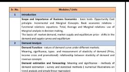
Business Economics - I, 01) Introduction, • Meaning, Scope and Importance of Business Economics, • Basic tools- Opportunity Cost principle- Incremental and, Marginal Concepts., • Basic economic relations - functional relations: equationsTotal, Average and Marginal relations- use of Marginal analysis, in decision making,, • The basics of market demand, market supply and equilibrium, price- shifts in the demand and supply curves and equilibrium

Page 3 :
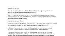
Meaning :, •, , Mc Nair and Meriam, “Business economic consists of, the use of economic modes of thought to analyze, business situations, , •, , Business Economics is a field in economics that deals, with issues such as business organisation, management,, expansion and strategy.

Page 4 :
Scope of Business Economics

Page 5 :
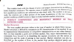
Basic Principles of Managerial, Economics, Economic concepts and analytical tools which can help to manager in his, decision making practices. It means the economics is most important, contributor in business economics., , Deceit in certain principles, , which are basic to the entire scope of business economics., , Principles, •, •, •, •, •, , The Incremental Concept, The Concept of Time Perspective, The Opportunity Cost Concept, The Discounting Concept, The Equi-marginal Concept

Page 6 :
•, , The Incremental Concept:, , The incremental concept is the most significant concept in economics and is, certainly the most frequently used in Business Economics. Incremental, concept is closely related to the marginal cost and marginal revenues of, economic theory., The two major concepts in this analysis are incremental cost and incremental, revenue. Incremental cost denotes change in total cost resulting from a, particular decision, whereas incremental revenue means change in total, revenue resulting from a decision of the firm., The incremental principle may be stated as follows:, A decision is obviously profitable one if ---(i) It increases revenue more than costs., (ii) It decreases some cost to a greater extent than it increases others., (iii) It increases some revenues more than it decreases others., (iv) It reduces costs more than revenues., Illustration: Suppose new order is estimated to bring in additional revenue of Rs. 5000/the cost are estimated in following cases, Case I, Case II, Labour - Rs. 1500, Labour – Rs. 1000, Material cost – Rs. 2000, Material cost – Rs. 2000, Overhead – Rs. 1800, Overhead - Rs. 500, Selling and administrative expenses – Rs. 700, Total cost – Rs. 6000

Page 7 :
• Opportunity cost, In Managerial Economics, the opportunity cost, concept is useful in decision involving a choice, between different alternative courses of action., Opportunity cost of a decision is the sacrifice of, alternatives required by that decision., The concept of opportunity cost implies three things:, 1. The calculation of opportunity cost involves the, measurement of sacrifices., 2. Sacrifices may be monetary or real., 3. The opportunity cost is termed as the cost of, sacrificed alternatives.

Page 8 :
• Equi-Marginal Principle, The principle states that an input should be allocated so that, value added by the last unit is the same in all cases. This, generalization is popularly called the Equi-marginal., Let us assume a case in which the firm has 100 unit of labour at, its disposal. And the firm is involved in five activities viz., А, В, C,, D and E. The firm can increase any one of these activities by, employing more labour but only at the cost i.e., sacrifice of other, activities., An optimum allocation cannot be achieved if the value of the, marginal product is greater in one activity than in another. It, would be, therefore, profitable to shift labour from low marginal, value activity to high marginal value activity, thus increasing the, total value of all products taken together., If, for example, the value of the marginal product of labour in, activity A is Rs. 50 while that in activity В is Rs. 70 then it is, possible and profitable to shift labour from activity A to activity B., The optimum is reached when the values of the marginal product, is equal to all activities. This can be expressed symbolically as, follows:, VMP = VMP = VMP = VMP = VMP, Where , VMP = Value of Marginal Product., L = Labour, LA, , LB, , LC, , LD, , LE

Page 9 :
• Discounting Principle, One of the fundamental ideas in economics is that a rupee tomorrow, is worth less than a rupee today. A simple example would make this, point clear., Suppose, you are offered a choice of Rs. 1,000 today or Rs. 1,000 next, year. Naturally, you will select Rs. 1,000 today. That is true because, future is uncertain. Let us assume you can earn 10 % interest during a, year., You may say that I would be indifferent between Rs. 1,000 today and, Rs. 1,100 next year i.e., Rs. 1,100 has the present worth of Rs. 1,000., Therefore, for making a decision in regard to any investment which will, yield a return over a period of time, it is advisable to find out its ‘net, present worth’. Unless these returns are discounted and the present, value of returns calculated, it is not possible to judge whether or not the, cost of undertaking the investment today is worth., The concept of discounting is found most useful in managerial, economics in decision problems pertaining to investment planning or, capital budgeting., The formula of computing the present value is given below:, V = A/1+i, where: V = Present value ; A = Amount invested Rs. 100 ; i = Rate of, interest 5 %; V = 100/1+.05 = 100/1.05 =Rs. 95.24

Page 10 :
Basic Economic Relations, • Functional Relation, Consider the relation between output, Q, and total, revenue, TR. Using functional notation, total revenue, is, TR = f(Q), Equation is read, “Total revenue is a function of, output.”, D=f(P), P=f(K,L), An equation is an expression of the functional, relationship or connection among economic, variables. It is a mathematical expression of two, variables, D=a-bpx

Page 11 :
• Total, Average, and Marginal Relations, Total, average, and marginal relations are very useful, in optimization analysis. Whereas the definitions of, totals and averages are well known, the meaning of, marginal needs further explanation., A marginal relation is the change in the dependent, variable caused by a one-unit change in an, independent variable., For example, marginal revenue is the change in total, revenue associated with a one-unit change in output, marginal cost is the change in total cost following a, one-unit change in output, marginal profit is the change in total profit due to a, one-unit change in output.

Page 12 :
• Total, Average, and Marginal Relationship under, Perfect Competition, 600, TR=P×Q, AR= TR÷Q, MR=ΔTR÷ΔQ, Quantity, , Price, (P), , Total, Revenue, (TR), , Average, Revenue, (AR), , Marginal, Revenue, (MR), , (Q), 1, , 100, , 100, , 100, , Nil, , 2, , 100, , 200, , 100, , 100, , 3, , 100, , 300, , 100, , 100, , 4, , 100, , 400, , 100, , 100, , 5, , 100, , 500, , 100, , 100, , • Perfect competition means large, number of buyers and sellers are, available in the market., • Products are homogeneous., AR and MR curve have horizontal slope, , 500, 400, TR, , 300, , AR, 200, , MR, , 100, 0, , 1, , 2, , 3, , 4, , 5

Page 13 :
• Revenue Curve under Imperfect Competition, When a firm is working under conditions of monopoly or, imperfect competition, its demand curve or AR curve is, less than perfectly elastic, the exact degree of elasticity, being different in different market situations depending, upon the number of sellers and the nature of product., In other words, the demand/AR curve has a negative, slope and the MR curve lies below it. This is because the, monopolist seller ordinarily has to accept a lower price, for his product, as he increases his sales., The Marginal Revenue (MR) must always be less than, Average Revenue (AR), because a falling price must, mean some loss on the sale of additional supply.

Page 14 :
TR=P×Q, AR= TR÷Q, MR=ΔTR÷ΔQ, Quantit, y, , (P), , Total, Revenue, (TR), , Average, Revenu, e, (AR), , Margina, l, Revenu, e, (MR), , 1, , 22, , 22, , 22, , 22, , 2, , 21, , 42, , 21, , 20, , 3, , 20, , 60, , 20, , 18, , 4, , 19, , 76, , 19, , 16, , 5, , 18, , 90, , 18, , 14, , 6, , 17, , 102, , 17, , 12, , 7, , 16, , 112, , 16, , 10, , 8, , 15, , 120, , 15, , 8, , 9, , 14, , 126, , 14, , 6, , 10, , 13, , 130, , 13, , 4, , (Q), , Price

Page 15 :
Revenue Curves under Oligopoly:, Under oligopoly market situation the number of sellers is, small. The price reduction or extension by one firm affects, the other firms. If a seller raises the price of his product,, others will not follow him. They know that by following the, same price, they can earn more profits. That producer, who, has raised the price, is likely to suffer losses because, demand of his product will fall.

Page 16 :
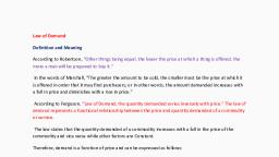
• Introduction to the Law of Demand:, The law of demand expresses a relationship, between the quantity demanded and its, price. Marshall’s words as “the amount, demanded increases with a fall in price,, and diminishes with a rise in price”. Thus, it expresses an inverse relation between, price and demand. The law refers to the, direction in which quantity demanded, changes with a change in price.

Page 17 :
These assumptions are:, (i) There is no change in the tastes and preferences of the, consumer;, (ii) The income of the consumer remains constant;, (iii) There is no change in customs;, (iv) The commodity to be used should not confer distinction, on the consumer;, (v) There should not be any substitutes of the commodity;, (vi) There should not be any change in the prices of other, products;

Page 18 :
Demand Schedule and Curve, Price, P, , Demand, Q, , 20, , 05, , 15, , 08, , 10, , 13, , 05, , 20

Page 19 :
Factors determining Demand, 1. Tastes and Preferences of the Consumers, 2. Incomes of the People, 3. Changes in the Prices of the Related Goods, 4. The Number of Consumers in the Market, 5. Changes in Propensity to Consume, 6. Consumers’ Expectations with regard to, Future Prices, 7. Income Distribution, 8. Price

Page 20 :
Shift in Demand Curve, A shift in the demand curve displays changes in, demand at each possible price, owing to change in one, or more non-price determinants such as the price of, related goods, income, taste & preferences and, expectations of the consumer. Whenever there is a, shift in the demand curve, there is a shift in the, equilibrium point also. The demand curve shifts in any, of the two sides:, Rightward Shift: It represents an increase in demand,, due to the favourable change in non-price variables, at, the same price., Leftward Shift: This is an indicator of a decrease in, demand when the price remains constant but owing to, unfavourable changes in determinants other than price.

Page 25 :
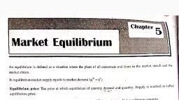
Market Equilibrium & Demand and, Supply Equilibrium, Definition: Market demand is the total amount of, goods and services that all consumers are, willing and able to purchase at a specific price, in a marketplace. In other words, it represents, how much consumers can and will buy from, suppliers at a given price level in a market., • Market equilibrium refers to the stage where, the quantity demanded for a product is equal to, the quantity supplied for the product., • The price when the quantity demanded is equal, to the quantity supplied for the product is, known as equilibrium price.

Page 27 :
Market Demand Curve

Page 28 :
Calculate Demand, D = a – bpx, Calculate Market Demand, MD = a + b + c + ….. + n, Calculate TR, AR and MR