Notes of Artisan, Fitter theory & Plumbing Theory & Mathematics & General Science & Engineering Drawing & Entrepreneurship & Life Skills & Communication skills CIB6832.pdf - Study Material
Page 2 :
Tel./Fax: +4205 4321 1134, E-mail:
[email protected], www.ta-service.cz, , PROGRAMME, Session A, A1, , Water Supply System - Field Measurement, A STUDY ON THE WATER AND ENERGY CONSUMPTION, IN NURSING HOMES FOR THE ELDERY, D. Nishina, S. Murakawa, H. Takata, T. Itai, Japan, , A2, , A STUDY ON BATHING BEHAVIOR AND HOT WATER USAGE, IN NURSING HOMES FOR THE AGED, A. Takaaze, S. Murakawa, D. Nishina, T. Itai, Japan, , A3, , DOMESTIC WATER CONSUMPTION AND ITS IRREGULARITY, , A4, , DOMESTIC HOT WATER CONSUMPTION IN ESTONIAN, APARTMENT BUILDINGS, , V. Suurkask, J. Säärekönno, Estonia, , A. Toodle, T.A. Köiv, Estonia, , A5, , A STUDY ON THE LOADS OF HOT WATER CONSUMPTION, IN HOUSES WITH THE HOT WATER STORAGE TANK SYSTEM, (PART 1) AN ANALYSIS OF THE HOT WATER USAGE AND THE, LOADS OF HOT WATER CONSUMPTION, N. Yamamoto, S. Murakawa, H. Takata,, H. Kitayma, Y. Hamada, M. Nabeshima, Japan, , A6, , A STUDY ON THE LOADS OF HOT WATER CONSUMPTION, IN HOUSES WITH THE HOT WATER STORAGE TANK SYSTEM, (PART 2) CALCULATIONS FOR THE LOADS OF HOT WATER, CONSUMPTION, , H. Takata, S. Murakawa, N. Yamamoto, H. Kitayma, Y. Hamada,, M. Nabeshima, Japan, , A7, , DEMAND ANALYSIS OF FRESH WATER SUPPLY FOR, A CHINESE RESTAURANT, K.W. Mui, L.T. Wong, M. K. Yeung, P.S. Hui, China, , Session B, , Water Supply System - Calculation Methods, Modelling, , B1, , CALCULATION FOR THE COLD AND HOT WATER DEMANDS, IN THE GUEST ROOMS OF CITY HOTEL, S. Murakawa, Y. Koshikawa, H. Takata, A. Tanaka, Japan, , B2, , MODELLING OF DOMESTIC HOT WATER TANK SIZE, FOR APARTMENT BUILDINGS II, L. Bárta, Czech Republic
Page 4 :
J.A. Swaffield, United Kingdom, , D7, , APPLICATION OF RENEUAL ASSESSMENT MODEL, IN BUILDING DRAINAGE SYSTEM, C. J. Yen, C. L. Cheng, K. C. Ho, W. L. Lee, Taiwan, , D8, , WATER- AND ENERGY SAVING ON WATER SYSTEMS, , Session E, , Testing Methods, Operation, Standardization, and Industrial Developments, , E1, , ASSESSMENT OF WATER SUPPLY AND DRAINAGE SYSTEMS, FOR AN HISTORICAL HAMMAM BY USING NON-DESTRUCTIVE, METHODS, , W.G. van der Schee, The Netherlands, , G. Disli, A. Tavukcuoglu, L. Tosun, E. N. Caner-Saltik, Turkey,, E. Grinzato, Italy, , E2, , IDENTIFICATION OF DEPLETED APPLIANCE TRAP SEALS, WITHIN THE BUILDING DRAINAGE AND VENTILATION, SYSTEM – A TRANSIENT-BASED TECHNIQUE, J.A. Swaffield, United Kingdom, , E3, , AN INDESTRUCTIBLE TESTING METHOD FOR AIR PRESSURE, DISTRIBUTION IN STACK OF BUILDING DRAINAGE SYSTEM, K. C. He, C. L. Cheng, L.T. Wong, P.S. Hui, W. R. Liao, Taiwan, , E4, , A STUDY ON THE TEST METHOD OF TRAP PERFORMANCE, , E5, , FLUSH QUALITY OF WC PANS, , E6, , STUDY ON THE CORROSION OF STEEL AND ZINC WITH, FLOW VELOCITY AND CORROSION CONTROL BY THE VACUUM, MEMBRANE DEAERATION SYSTEM IN TAP WATER ANALYSIS, ON THE CORROSION OF STEEL AND ZINC AND GALVANIC, CORROSION OF GUNMETAL/ GALVANIZED STEEL PIPES, , K. Sakaue, M. Kamata, Y Zhang, Japan, , T. Seelig, Ch. Henke, M. Demiriz, Germany, , T. Yamate, S. Murakawa, Japan, , E7, , STUDY OF PATHOLOGIES IN WATER AND DRAINAGE, PLUMBING SYSTEMS, S. V. de Amorim, A. P. da Conceiçăo, L.M. Ferrante,, Ry. De V. Guimarăes, Brazil, , E8, , PRESENT STATE AND FUTURE CHALLENGE ON INSTALLATION, NUMBER OF THE SANITARY FIXTURE, H. Kose, Japan, , E9, , MYTHS AND LEGENDS: DEVELOPMENTS TOWARDS MODERN, SANITARY ENGINEERING, M. Gormley, United Kingdom
Page 5 :
E10, , ACTIVE AIR PRESSURE SUPPRESSION OF DRAINAGE SYSTEMS, - FROM RESEARCH TO THE MARKETPLACE, S. White, United Kingdom, , Session F, , Drainage Systems – Hydraulic, , F1, , INFLUENCE OF UNSTEADY FRICTION ON TRAP, SEAL DEPLETION, J.A. Swaffield, United Kingdom, , F2, , STUDIES OF A TESTING METHOD FOR AIR ADMITTANCE VALVE, CHARACTERISTICS AND A DESIGN METHOD FOR VENT PIPES, M. Otsuka, J. Ma, Japan, , F3, , INFLUENCE OF FLOW CAPACITY ON THE VENT SYSTEM, OF A DRAINAGE SYSTEM GRASP OF THE VENTILATION CAPACITY, BY FIXTURE DRAINAGE LOAD, N. Honngo, M. Otsuka, K. Kawasaki, Japan, , F4, , A NUMERICAL APPROACH TO INVESTIGATE SOLID TRANSPORT, CHARACTERISTICS IN WASTE WATER DRAINAGE SYSTEMS, A. Öngören, B. Meier, Switzerland, , F5, , EXPERIMENTAL STUDY OF DRAINAGE CHARACTERISTICS, OF WATER SAVING TOILET BOWLS AND TRANSPORT, PERFORMANCE EVALUATION, T. Ishii, M. Otsuka, Japan, , F6, , NOVEL SIPHONIC ROOF DRAINAGE DEVICES, , F7, , THE PRIMING FOCUSSED DESIGN OF SIPHONIC ROOF DRAINAGE, , F8, , A STUDY ON THE SIPHON DRAINAGE SYSTEM, , D.P. Campbell, United Kingdom, , S. Arthur, United Kingdom, , N. Tsukagoshi, K. Sakaue, Japan
Page 6 :
A Study on the Water and Energy Consumption in, Nursing Homes for the Elderly, , A1), , Daisaku Nishina (1), Saburo Murakawa (2),, Hiroshi Takata (3) and Takanori Itai (4), (1)
[email protected], (2)
[email protected], (3)
[email protected], (4)
[email protected], (1), (2), (4) Graduate School of Engineering, Hiroshima Univ., Japan, (3) Graduate School of Educating, Hiroshima Univ., Japan, , Abstract, Recently, Japan is facing fast-aging society according to the birthrate declining, and the improvement in life expectancy. In parallel with the change of social condition,, the new care styles, such as day-care, home care, etc. have been introduced. As for, nursing homes for the elderly, not only the quantitative expansion of homes, but also the, qualitative enhancement of facilities and equipments are required more in order to, improve quality of life of the residents., However, in regards to the new type of nursing homes, the data is not sufficient for, the planning and designing of building systems. The purpose of this study is to clarify, the actual condition of water and energy consumption of the home and to obtain the, fundamental data for design. Therefore, the measurements of hot and cold water and, energy consumption were carried out in two nursing homes called Facility T and, Facility S. The measurement periods were approximately two weeks in winter and one, week in summer. Because Facility T and Facility S utilize electricity and liquefied, petroleum gas respectively, as an energy source of hot water supply, Facility T has a, heat storage unit with heat pump and Facility S has a boiler and a hot water storage, tank. There are dining rooms, recreation rooms, bathrooms and private rooms for, residents in both facilities. Well water is used for flushing the toilets in both facilities,, and Facility S uses well water for the bathrooms., In this paper, the daily and hourly consumption of cold and hot water in each, season are shown and the relation between the water consumption and the daily, schedule of the residents and the caregivers in two facilities are examined., , 3
Page 7 :
Keywords, Elderly Nursing Home, Hot Water Consumption, Cold Water Consumption,, , 1. Introduction, The purpose of this study is to collect basic information of current equipment design, of elderly nursing homes aiming at energy conservation planning. The authors measured, the consumption of cold and hot water and energy consumption at two elderly nursing, homes called Facility T and Facility S in order to understand actual usage of cold and, hot water. In this study, the facility overview (Facility T and Facility S) shall be, reported to compare and investigate the loads of cold and hot water usage in both, facilities., , 2. Outline of the investigation, 2.1 Outline of the facilities, The facilities surveyed are Facility T an all-electric facility and Facility S which is, on the same scale as Facility T but uses a gas heat source. Facility T and S are located in, the northeast and the northwest of Hiroshima prefecture, respectively. Facility T is an, elderly nursing home with a care house for the elderly who do not need any help., Facility S is a special elderly nursing home, also a care house, short stay center and a, day service center are attached to this facility., Table 1 shows the overview of each facility. Both facilities have a central hot water, supply system and in both facilities hot water is supplied to the common areas such as, the bathing room and laundry room. Facility T has two bathrooms each for the elderly, nursing home and the care house. Also, Facility S has two bathrooms each for the, special elderly nursing home, the care house and the day service center. Facility T, utilizes city water as the, Table 1 Overview of two facilities, Facility T, Building use, Total floor area (• ), Number of stories, Location, Capacity of people, Heat source for hot water supply, Hot water apparatus, , Hot water storage tank • L•, , Nursing home, Care house, Short stay, 3,797.86, 3, Hiroshima pref.Syobara city, 51.00, Electricity, Heat storage unit for hot water supply, Performance of heating • kW•, Electric capacity • kW•, 10,200, , 4, , Facility S, 28 Special elderly nursing home, 20 Care house, 3, 4,043.90, 2, Hiroshima pref.Kitahiroshima city, 77.00, , 50, 27, , Gas, Hot water heater, 90 Performance of heating • kJ/h•, 1,465,100, 33 Hot water consumption (L/h), 6,500 (0°C→50°C), 3, 17.2(LPG•, Fuel consumption • m /h•, 4,000
Page 8 :
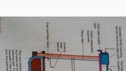
Cold water (City water), Cold water (Well water), , Hot water (Supply), Hot water (Return), , Heat exchager, , Care house Elderly nursing home, 7, M T, , Heat pump, , Kitchen, Cold water, (City water), , 5 6, M, , M4, , Cold water, (Well water), , T, , 1, , Electric, hot water, heater, , Heat storage unit, for hot water supply, , T, , 10, , M T, T, , 13, , M T, , 15, , M T, , 8, 9, 11, 12, 14, , Bathing rooms,, Laundry rooms, etc., Bathing rooms,, Laundry rooms,, Private rooms, etc., , 16, , 3, , M T, , 2, , Toilet, , M, , Facility T, , M, T, , Gas, hot water, boiler, , Ultrasonic flow meter, Temperature sensor, , Bathing room of, day service center, , Hot water, storage tank, , 4M, , 5, , M, , 10, , M, , Kitchen, 6, , 7M, , T, , 8, , M, , Cold water 3M, (City water), , 9, , M, , Bathing rooms,, Private rooms,, etc., Bathing rooms,, Private rooms,, Dining, etc., Bathing rooms,, Private rooms,, etc., , Cold water 1 2, M, T, (Well water), , Facility S, , Figure 1 Cold and hot water supply system of two facilities, Table 2 Measurement items of two facilities, Facility T, Number, 1, Total flow rate of cold water (City water), 2, Total flow rate of cold water (Well water), 3, Temperature of cold water (City water), 4, Flow rate of cold water for a kitchen, Flow rate of hot water for a kitchen, 5, Temperature of hot water for a kitchen, 6, 7, Flow rate of hot water for heating up (Supply), Bathing rooms, 8, Temperature of hot water for heating up (Supply), of a care house, 9, Temperature of hot water for heating up (Return), 10, Bathing rooms Flow rate of hot water for heating up (Supply), of a elderly, 11, Temperature of hot water for heating up (Supply), nursing home Temperature of hot water for heating up (Return), 12, 13, Total flow rate of hot water (Supply), 14, Temperature of hot water (Supply), 15, Total flow rate of hot water (Return), 16, Temperature of hot water (Return), * The number corresponds to the number of measuring point in Figure 1., , 5, , Facility S, Total flow rate of cold water (Well water), Temperature of cold water (Well water), Total flow rate of cold water (City water), Flow rate of hot water for bathing rooms for day service, Total flow rate of hot water (Supply), Temperature of hot water (Supply), Flow rate of hot water for a kitchen (Supply), Flow rate of hot water for a kitchen (Return), Flow rate of hot water except for a kitchen (Return), Total flow rate of hot water (Return)
Page 9 :
source of the hot water supply while Facility S utilizes well water. In Facility T, an, electric water heater is equipped to each private room and to the kitchen. In Facility S,, an electric water heater is equipped in each dining hall. In this research, these individual, hot water supply system had been excluded from the measurement. However, the, kitchen electrical water heater in Facility T was included., 2.2 Outline of the measurements, In this study, wide-ranging measurements were taken during the summer and winter, months. The measurement items were divided into three groups, the energy, consumption such as the electricity and gas used, the cold and hot water consumption, and the indoor thermal environment. This paper shows the outline of the cold and hot, water consumption measurements., Figure 1 shows the cold and hot water supply system along with the major, measurement points. Table 2 shows the measurement items for each facility. In regards, to the measurement item 7 and 10 in Facility T, the water supply is circulated with, constant flow for the bathing room water heat up, thus the measurement was, implemented only during the winter. Using an ultrasonic flow meter to measure water, flow and using a surface temperature sensor for water temperature measurements,, sequential measurements were recorded automatically at one-minute intervals. The, period of the measurements of the cold and hot water consumption in both facilities, were 1 to 2 weeks for each season in 2004 and the same period was used for the energy, consumption measurements., Table 3 shows the measurement period and statistics of the outside air temperature, during the same period. Based on this table, it can be seen that the temperature in winter, is slightly lower at Facility T compared to Facility S. The average winter temperature at, Facility T is –0.6 °C, and the temperature remains below zero for the entire, measurement period. In particular, the lowest average temperature per day of –5.1 °C, was recorded on January 22. On the other hand, the summer time shows the opposite, trend as Facility T has a higher temperature than Facility S. However, this tendency may, be affected by the measurement period., Table 3 Measurement periods and outside air temperature, Standard, Maximum, Average, value[°C] deviation[°C] value[°C], -0.6, 2.1, 2.5, 25.0, 1.9, 26.9, 2.2, 1.7, 4.9, 23.7, 2.4, 25.9, , Period of measurement, Facility T, Facility S, , Winter, Summer, Winter, Summer, , 16 1.2004 - 29 1.2005, 25 8.2004 - 2 9.2004, 3 2.2004 - 15 2.2004, 15 9.2004 - 23 9.2004, , Minimum, value[°C], -5.1, 21.2, -0.3, 19.3, , Table 4 Temperatures of hot and cold water, Cold water, (City water) [°C], Facility T, Facility S, , Winter, Summer, Winter, Summer, , Cold water, (Well water) [°C], , Hot water storage, tank [°C], , 9.4, 21.5, 16.0, 22.3, , 52.2, 55.1, 55.2, 55.6, , 4.3, 24.4, 10.8, 28.2, , 6, , Hot water for a, kitchen[°C], 71.0, 75.3, -
Page 10 :
3. The consumption of cold and hot water, 3.1 Temperatures of cold and hot water, Table 4 shows the average temperature of the cold and hot water for each season., Hot water storage tank temperature indicates when the water is supplied from the tank, to the common area, and the temperature of the hot water for a kitchen at Facility T, indicates when the water is supplied from the electric water heater to the kitchen. The, hot water average temperature is based on the data when the water heater operates., From the above table, it can be seen that the hot water storage tank supplies water at 50, °C for each season., 3.2 Daily consumption of cold and hot water, Table 5 shows the statistics of daily consumption of the cold and hot water in both, facilities. The cold water consumption figures shown in table 5 are the combined values, of both the city water and well water, except for the hot water. Also, the hot water, Table 5 Daily consumption of hot and cold water, Facility T, , Actual value, Basic unit, , Winter, 31.292, 1.983, 34.062, 26.631, 11.573, 1.423, 13.843, 8.827, 6.106, 0.571, 6.945, 4.678, 5.556, 1.010, 6.898, 3.856, 8.239, 0.522, 8.969, 7.012, 3.047, 0.375, 3.645, 2.324, 1.608, 0.150, 1.829, 1.232, 1.463, 0.266, 1.816, 1.015, , Total of cold and Avarege value, hot water, Standard deviation, consumption Maximum value, 3, Minimum value, [m ], Avarege value, Hot water, Standard deviation, 3, consumption [m ] Maximum value, Minimum value, Avarege value, For a kitchen Standard deviation, 3, Maximum value, [m ], Minimum value, Avarege value, For bathing Standard deviation, 3, rooms [m ] Maximum value, Minimum value, Total of cold and Avarege value, hot water, Standard deviation, consumption Maximum value, 2, Minimum value, • L/m • d•, Avarege value, Hot water, Standard deviation, consumption, Maximum value, 2, [L/m • d], Minimum value, Avarege value, For a kitchen Standard deviation, 2, [L/m • d] Maximum value, Minimum value, For bathing Avarege value, Standard deviation, rooms, Maximum value, 2, [L/m • d], Minimum value, , 7, , Summer, 31.464, 2.111, 34.884, 27.976, 11.742, 1.781, 14.414, 9.037, 5.881, 0.567, 6.761, 5.141, 5.861, 1.377, 8.261, 3.801, 8.285, 0.556, 9.185, 7.366, 3.092, 0.469, 3.795, 2.379, 1.548, 0.149, 1.780, 1.354, 1.543, 0.363, 2.175, 1.001, , Facility S, Winter, 30.791, 9.506, 41.566, 15.825, 13.661, 5.750, 21.183, 4.819, 5.981, 2.018, 9.833, 2.567, 7.680, 4.331, 14.739, 1.576, 7.614, 2.351, 10.279, 3.913, 3.378, 1.422, 5.238, 1.192, 1.479, 0.499, 2.432, 0.635, 1.899, 1.071, 3.645, 0.390, , Summer, 27.613, 9.819, 39.694, 13.463, 7.859, 4.671, 15.013, 1.906, 2.915, 0.839, 4.297, 1.430, 4.944, 4.136, 11.750, 0.377, 6.828, 2.428, 9.816, 3.329, 1.943, 1.155, 3.713, 0.471, 0.721, 0.207, 1.063, 0.354, 1.223, 1.023, 2.906, 0.093
Page 11 :
12, , Hot water consumption, , Cold water consumption, , Hot water consumption, , Cold water consumption, , 10, , 10, , 8, , 8, , 6, , 6, , 4, , 4, 2, , Facility T, , 0, , 9/15, 9/16, 9/17, 9/18, 9/19, 9/20, 9/21, 9/22, 9/23., , 8/25, 8/26, 8/27, 8/28, 8/29, 8/30, 8/31, 9/1, 9/2., , 1/16, 1/17, 1/18, 1/19, 1/20, 1/21, 1/22, 1/23, 1/24, 1/25, 1/26, 1/27, 1/28, 1/29, , 2, 2/3, 2/4, 2/5, 2/6, 2/7, 2/8, 2/9, 2/10, 2/11, 2/12, 2/13, 2/14, 2/15, , Basic unit of cold and hot water, consumption, [L/ d], , 12, , 0, , Basic unit of cold and hot water consumption, [L/ d], , consumption for bathing rooms defines the amount of the hot water supplied by the, central system except for the hot water consumption for a kitchen. The laundry rooms of, Facility T and the laundry and guest rooms of Facility S are included in the figure of the, bathing rooms. In addition, for both facilities, floor area (m2) is used to calculate the, consumption per square meter as the basic unit of consumption., As for the basic unit of total of cold and hot water consumption, both facilities do, not show major differences on a daily average. However, based on the standard, deviation, Facility S shows large variation as a major difference was found between the, maximum and minimum values of daily consumption, though Facility T does not show, such a deviation. On the other hand, when comparing winter and summer averages of, Facility S and Facility T, the facilities show small changes in average or deviation. Each, facility also shows almost the same way of using water in summer and winter., In regards to the hot water consumption, in Facility T, the standard deviation is, smaller than Facility S and there is a small difference of standard deviation between the, seasons in each facility. Also it can be considered as the similar tendency for total, consumption of cold and hot water. In Facility S, there is a difference in the standard, deviation between the seasons. In the summer, hot water consumption is reduced to, 60% of the winter consumption., In the hot water consumption for bathing rooms, the standard deviation is higher, compared with the hot water consumption for a kitchen. This tendency can be seen in, both facilities and it may depend on weekly shower or bath time schedule. The decrease, of the hot water usage during summer in Facility S can be seen in the hot water, consumption for a kitchen and bathing rooms as well, but it is expected that the water, for the dish washing in the kitchen and cleaning the bathing rooms may have changed to, cold water from hot water in the summer., Figure 2 shows the daily variation of the basic unit of cold and hot water, consumption in Facility T and Facility S respectively. As for the percentage of the hot, water consumption of the total consumption of cold and hot water, in Facility T, it, accounts for 37.6% in winter and 37.3% in summer. Also, in Facility S, it accounts for, 44.4% for winter and 28.5% for summer. As above, Facility T shows a stabilized, percentage for both cold and hot water consumption, however, as stated previously,, there are major changes in cold and hot water usage in Facility S. There are bathing, rooms on the 1st and 2nd floors in Facility S. Water is supplied to the 1st floor bathing, , Facility S, , Figure 2 Basic unit of daily consumption, , 8
Page 12 :
room 2 or 3 times a week in both winter and summer. Water is supplied to the 2nd floor, bathing room 4 times a week during winter and approximately 3 times a week during, summer. These facts may affect on the consumption., Figure 3 shows the percentage of the hot water consumption for bathing rooms and, a kitchen for each season in both facilities. The hot water consumption for a kitchen in, Facility T accounts for 50% of the total consumption of hot water and in Facility S it, accounts for 40% of total. Also, these ratios in both facilities show small variation for, each season., 3.3 Hourly consumption of cold and hot water, Table 6 shows the cold and hot water consumption per hour in both facilities. The, average of hourly consumption of hot water is calculated during a period of 20 hours, from 4 am to 11 pm. As for the peak time of hot water in Facility T, the peak, Winter, Summer, 0%, , 25%, , 50%, , 75% 100% 0%, , 25%, , Facility T, , 50%, , 75% 100%, , Facility S, , For bathing rooms, , For a kitchen, , Figure 3 Percentage of hot water consumption for a kitchen and bathing rooms, Table 6 Hourly consumption of cold and hot water, Facility T, , Actual value, Basic unit, , Average value [L/h], Total of cold and hot Maximum hourly consumption[L/h], water consumption Peak ratio, Time zone of peak occurrence [hour], Average value [L/h], Hot water, Maximum hourly consumption[L/h], consumption, Peak ratio, Time zone of peak occurrence [hour], Average value [L/h], Maximum hourly consumption[L/h], For a kitchen, Peak ratio, Time zone of peak occurrence [hour], Average value [L/h], For bathing Maximum hourly consumption[L/h], rooms, Peak ratio, Time zone of peak occurrence [hour], Total of cold and hot Average value [L/m\2• h], water consumption Maximum hourly consumption [L/m2• h], 2, Hot water, Average value [L/m • h], 2, consumption, Maximum hourly consumption [L/m • h], 2, h], value, [L/m, Average, •, For a kitchen, 2, Maximum hourly consumption [L/m • h], For bathing Average value [L/m2• h], 2, rooms, Maximum hourly consumption [L/m • h], , 9, , Winter, Summer, 1292.34 1311.02, 2755.00 4739.30, 0.09, 0.15, 7, 1, 527.76, 585.77, 2266.00 3196.00, 0.16, 0.25, 11, 20, 288.52, 292.81, 1015.00 1065.00, 0.17, 0.17, 11, 18, 277.37, 292.96, 1950.00 3196.00, 0.39, 0.52, 20, 20, 0.340, 0.345, 0.725, 1.248, 0.139, 0.154, 0.597, 0.842, 0.076, 0.077, 0.267, 0.280, 0.073, 0.077, 0.513, 0.842, , Facility S, Winter, Summer, 1282.94 1150.56, 6309.00 8096.00, 0.16, 0.20, 8, 11, 682.80, 392.95, 3684.00 4141.00, 0.23, 0.32, 8, 5, 299.04, 145.75, 2167.00 1222.00, 0.22, 0.47, 9, 5, 383.76, 247.20, 2865.00 3441.00, 0.30, 0.36, 8, 5, 0.317, 0.285, 1.560, 2.002, 0.169, 0.097, 0.911, 1.024, 0.074, 0.036, 0.536, 0.302, 0.095, 0.061, 0.708, 0.851
Page 13 :
Hot water consumption [L/h], , consumption for a kitchen occurs at 11:00 am when lunch preparation starts. The peak, time for bathing rooms is 8:00 pm, as that is the bathing room cleaning time. As for, Facility S, the peak time of hot water consumption is in the morning when the water is, supplied to the bathing room for filling bath full. In the peak percentage, the value of the, hot water consumption for bathing rooms is higher than others in both facilities., Secondarily, Figure 4 and 5 show the changes of hourly consumption of hot water in, both facilities during summer and winter. According to the results, the variations of hot, water consumption are clarified. As stated previously, as the variation of daily, consumption of hot water is large in Facility S, two and three patterns are divided in, winter and summer, respectively., In Facility T, based on the results in winter, the hot water for bathing room was used, for backwashing of an extraction filter at 6:00 am and 12:00 pm and also, the water was, used for skim removal by intentionally overflowing the water in order to clean the bath, tub in the care house at 10:00 am. The skim removal was implemented after 8:00 pm, when the bathing room was closed, and these are the times when the hot water is used, the most. As for the hot water for a kitchen, similar amount of water is used during, breakfast (5-8 am), lunch (11 am-2 pm) and dinner (5-7pm). These trends stated above, 2000, For bathing rooms, , 1600, , For a kitchen, , 1200, 800, 400, 0, 0, , 2, , 4, , 6, , 8 10 12 14 16 18 20 22, , 0, , 2, , 4, , 6, , 8 10 12 14 16 18 20 22, , Winter, , Summer, , Hot water consumption [L/h], , Figure 4 Hourly consumption of hot water in Facility T, 4000, 3500, , For bathing rooms, , For a kitchen, , 3000, 2500, 2000, 1500, 1000, 500, 0, 0, , 3, , 6, , 9, , 12, , 15, , 18, , 21, , 0, , 3, , Hot water consumption [L/h], , Winter 1 (n=7), , 6, , 9, , 12, , 15, , 18, , 21, , Winter 2 (n=6), , 4000, 3500, 3000, 2500, 2000, 1500, 1000, 500, 0, 0, , 2, , 4, , 6, , 8 10 12 14 16 18 20 22, , 0, , 3, , 6, , 9, , 12, , 15, , 18, , 21, , 0, , 2, , 4, , 6, , 8 10 12 14 16 18 20 22, , Summer 1 (n=4), Summer 2 (n=2), Summer 3 (n=3), Figure 5 Hourly consumption of hot water in Facility S, , 10
Page 14 :
can be seen during the summer time as well. Additionally, the hot water consumption, for cleaning the bathing room at 8 pm is more significant in summer., On the other hand, the variation for Facility S is divided into several patterns. The, winter water usage is broken into 2 patterns. The pattern Winter 1 is the days when the, hot water was supplied to the day service bathing room for filling up water in the, bathtub. The pattern Winter 2 is the days when no hot water was supplied to the day, service bathing room. The summer is broken into 3 patterns with Summer 1 and 2 the, same as Winter 1 and 2 respectively, but in addition, Summer 3 is for the days when, there was no bathing room usage., As for the period Winter 1, the day service user used the bathing room on Monday,, Tuesday, Thursday and Saturday, on these days hot water is supplied to fill up water in, the bathtub at 8 am. Also in the morning, there were lifting shower times and bathing, with mechanical bathtubs for the special elderly nursing home and bathing in the day, service center. In the afternoon, the bathing room was used for the care house until 4 pm, so that the hot water consumption per hour goes up during these periods. From 8 pm to, 9 pm, hot water was used for cleaning the bathing room. For the hot water consumption, per hour for a kitchen, the time when hot water is used is different from Facility T,, however a similar tendency can be found that the hot water consumption increases, during three different periods in a day. In Winter 2, there was bathing time for the, special elderly nursing home and for the care house in the morning and the afternoon, respectively, but the consumption of hot water is low. Also, Winter 2 includes Sunday, , Table 7 Daily heat amounts for hot water, Facility T, , Heat load, [MJ/d], Actual value, , For a kitchen, [MJ/d], For bathing, rooms, [MJ/d], Heat load, 2, , [MJ/m • d], Basic unit, , For a kitchen, 2, [MJ/m • d], For bathing, rooms, 2, [MJ/m • d], , Winter, 2640.65, 350.27, 3038.25, 2099.19, 1526.04, 322.85, 1829.42, 850.92, 1134.47, 210.81, 1417.99, 787.53, 0.695, 0.092, 0.800, 0.553, 0.402, 0.085, 0.482, 0.224, 0.299, 0.056, 0.373, 0.207, , Average value, Standard deviation, Maximum value, Minimum value, Average value, Standard deviation, Maximum value, Minimum value, Average value, Standard deviation, Maximum value, Minimum value, Average value, Standard deviation, Maximum value, Minimum value, Average value, Standard deviation, Maximum value, Minimum value, Average value, Standard deviation, Maximum value, Minimum value, , 11, , Summer, 1972.86, 253.74, 2349.91, 1558.10, 1212.32, 91.68, 1320.54, 1065.96, 760.55, 180.04, 1077.47, 492.13, 0.519, 0.067, 0.619, 0.410, 0.319, 0.024, 0.348, 0.281, 0.200, 0.047, 0.284, 0.130, , Facility S, Winter, 2860.08, 1178.97, 4289.83, 1007.28, 1263.74, 422.95, 2062.12, 533.39, 1596.34, 882.14, 2947.87, 338.24, 0.707, 0.292, 1.061, 0.249, 0.313, 0.105, 0.510, 0.132, 0.395, 0.218, 0.729, 0.084, , Summer, 1011.74, 588.29, 1915.18, 250.33, 384.31, 110.94, 572.35, 187.37, 627.42, 518.24, 1486.13, 50.17, 0.250, 0.145, 0.474, 0.062, 0.095, 0.027, 0.142, 0.046, 0.155, 0.128, 0.367, 0.012
Page 15 :
when there was no bathing time., For Summer 1, there were lifter shower and bathing with mechanical bathtubs in, the morning. The bathtub in the day service center is filled with water at 11 am. In, Summer 2, hot water was supplied into bathtubs located on the 1st floor and hot water, was used in the care house bathing room at 10 am. In Summer 3, the bathing room, usage is almost none and water is used only for the kitchen. As above, the hourly, consumption of hot water changes drastically for the each pattern in Facility S so that, Summer 1 and Winter 1 which show high water consumption need to be investigated in, order to collect information regarding the equipment design., 3.4 Heat consumption, Table 7 shows the statistics of hot water heat amount per day in Facility T and, Facility S. As the water source for the hot water supply is different between Facility T, and Facility S, the cold water temperature in Facility T is used for the heat amount, calculation in order to compare the heat consumption in both facilities., As for the hot water heat consumption, Facility T shows average 2640.65 [MJ/d], during winter time and 1972.86 [MJ/d] during summer time. In Facility S, the winter, time and summer time usage are 2860.08 [MJ/d] and 1011.74 [MJ/d], respectively. The, heat amount is significantly reduced during summer time in Facility S., , 4. Conclusion, In this study, the characteristics of cold and hot water usage are clarified by, comparison of both facilities based on the statistics of daily and hourly consumption of, cold and hot water, and supplied heat amount in two seasons., As for the daily total consumption of cold and hot water, the basic units are, approximately the same between two facilities during summer and winter. In the daily, consumption of hot water, the similar tendency in both facilities is obtained, except the, hot water consumption during summer in Facility S, as the purpose of hot water usage, changes. Furthermore, each percentage of the consumption for a kitchen and for bathing, rooms accounts for 50 % respectively in total hot water consumption., In the standard deviation of daily consumption of cold and hot water, the difference, between two facilities is significant. In Facility S, the consumption of hot water varies, day by day, because the usage of the bathing rooms changes on each day. The result can, be confirmed based on the correspondence between the hourly hot water consumption, and the bathing room schedule., , 5 Acknowledgments, The authors wish to express their gratitude for the great cooperation by people who, involved in the nursing homes., , 12
Page 16 :
6 References, 1. T. Itai, et al. (2007). A study on the Energy Consumption of Welfare Facilities for, aged, Part 5 An Analysis of the Loads of Cold and Hot Water Consumption., Proceedings of AIJ Tyugoku Chapter Architectural Research Meeting, Vol. 30, 445448, 2. M. Miyoshi, et al. (2005). A study on the Energy Consumption of Welfare Facilities, for aged, Part 3 Measurement Result of the Cold and Hot Water. Proceedings of AIJ, Tyugoku Chapter Architectural Research Meeting, Vol. 28, 489-492, , 7 Presentation of Author, Daisaku Nishina is an Associate Professor at Gr aduate School of, Engineering, Hiroshima University. His special field is the planning, of water supply system and water environment for people, , 13
Page 17 :
14
Page 18 :
A2) A Study, , on Bathing Behavior and Hot Water Usage, in Nursing Homes for the Aged, A. Takaaze (1), S. Murakawa (1), D. Nishina (1), T. Itai (1), (1)Graduate School of Engineering, Hiroshima University, 1-4-1 Kagamiyama, Higashi-Hiroshima City, 739-8527, Japan, , Abstract, In Japan, the number of elderly people who need care in daily life has been increasing for, the past 30 years and this trend is expected to continue. In order to ensure that they have, comfortable and fulfilling lives, the construction of nursing homes for them and the, introduction of appropriate fixtures into the homes are required., Many elderly people in nursing homes need help when they take a bath. Their bathing, styles are different from people who do not need care. In such homes, a lot of hot water is, consumed in bathrooms and this consumption affects greatly the energy consumption of, the hot water supply system in a whole building. However, the actual conditions of the, consumption and the usage behavior of hot water have not been revealed yet, though it is, important to design the appropriate system in nursing homes. Therefore, the purpose of, this study is to clarify these conditions and analyze the relationship between consumption, and behavior. This is based on the measurements and the observation surveys given in, bathrooms of an actual nursing home which was chosen in the east area of Hiroshima., The quantity and the temperature of cold and hot water in each faucet were measured, continuously for each bathing. At the same time, the actions of elderly people and the, caregivers during the process of bathing were observed and recorded by researchers that, stayed in the rooms. These measurements and surveys were carried out for about a week, in three seasons. Additionally, questionnaires for the aged and the caregivers were, conducted following the period of observational study., In this paper, the behavioral process in which bathing occurred were defined based on the, results of the observation. The time length and the total water consumption of bathing per, capita were clarified and the temperature and the water consumption in each action were, identified., , 15
Page 19 :
Keywords, Assisted bathing, Nursing home, Water consumption, Bathing behavior, , 1 Introduction, Japanese society has been aging because of the declining birthrate and death rate as well, as increasing life expectancy. The number of people who are identified as people who, need public nursing care by elderly care insurance system is also increasing. This, phenomenon raises awareness of people for nursing care systems and nursing care, facilities. People have recently put much emphasis on satisfaction of not only quantity of, facilities but various and high quality nursing care. In recent trend, efficient aggregation, care replaced private care which considered individual cases in many nursing care homes., At the same time, improvement of nursing care facilities and functions becomes, important to give elderly people high quality care services and comfortable life spaces., Many elderly people in nursing homes need help when they take a bath. Their bathing, styles are different from people who do not need care. In such homes, a lot of hot water is, consumed in bathrooms and this consumption affects greatly the energy consumption of, the hot water supply system in a whole building. However, the actual conditions of the, consumption and the usage behavior of hot water have not been revealed yet, though it is, important to design the appropriate system in nursing homes. Therefore, the purpose of, this study is to clarify these conditions and analyze the relationship between consumption, and behavior., , 2 Outline of the investigation, 2.1 Outline of the measurements, Two bathrooms of the nursing home in the east area of Hiroshima were surveyed. One is a, share bathroom, the other is a private bathroom. The floor plans of the bathrooms and the, summary of the facilities which is in the bathrooms are shown in Figure 1 and Table 1., There are three different bathtubs, (a mechanical bathtub, a large bathtub and a small, bathtub) in the share bathroom. Wash spaces are arranged for each bathtub. The private, bathroom has one bathtub for single use. Floor area of private bathroom is one fifteenth of, the share bathroom and it manages to allow two people to come in., The measurements were carried out for about a week each in three seasons. Table 2 shows, the period of the measurements. Figure 2 shows the distribution diagram of cold and hot, water pipes and the position of measuring instruments. In order to figure out cold and hot, water consumption at each shower, flow meters were put in not only main pipes but, branch pipes and measured at 1-second intervals. Temperature sensors were put in the, inside of cold and hot water pipes and measured at 2-second intervals. Warm water made, up of cold and hot water is used at each showerhead or mixed water faucet., Characteristics of the warm water usage are revealed in this paper and it is called water, , 16
Page 20 :
hereinafter., , Shower, , C, D, , Mixed Water Faucet, , b, , Cold Water Faucet, , Large Bathtub, Small Bathtub, a, , 0.2, , A, , 2, , 0 0.5, , Private Bathtub, , Mechanical, Bathtub, , B, , 1, , Share Bathroom, , Private Bathroom, , Figure 1 – Bathroom Plans, Table 1 – Bathroom Facilities, Shear Bathroom, Bathroom Space, , 43.7, , Dressing Space, , 25.3, , Capacity, of Bathtub, , Facilities, , Private Bathroom, 2.8, 3.2, , Mechanical Bathtub, , 560, , Large Bathtub, , 1400, , Small Bathtub, , 900, , Private Bathtub, , 320, , Mixed Water Faucet, , 2, , Mixed Water Faucet, , 1, , Shower connected to mechanical bathtub, , 4, , Shower, , 1, , Shower, , 4, , Cold Water Faucet, , 1, 10:00, 13:30, , Hours, , 12:00, 15:30, , 10:00, , 12:00, , Table 2 – Periods of Measurements, The Period of, Measurements, T, T, , Cold Water Faucet, , Summer, , 5/ 8/ 2006, , Autumn, , 11/ 10/ 2006, , 18/ 10/ 2006, , Winter, , 15/ 12/ 2006, , 22/ 12/ 2006, , M, M, , M, , M, , 11/ 8/ 2006, , Mechanical Bathtub,, 4 showers, Mixed Water Faucet, , Shower A, , M, , Shower B, , Shower, , Mixed Water Faucet a, M, M M, M, , Mixed Water Faucet b, , T T, T, T, , M, , Shower C, , M, M, T, , Private Bathroom, Shower D, , T, , Share Bathroom, , Ho t Wa, ter Supply, Hot, Water, Supply Pipe, Pipe, , M, , Flo w Sen, sor, Flow, Sensor, , Cold Water Supply Pipe, , T, , Temperature Sensor, , Figure 2 – Cold and Hot Water Supply System, , 17
Page 21 :
2.2 Characteristics of bathing styles and elderly people, Observational investigation on the actual bathing situation was carried out in the, bathrooms at the same time of measurements. Respondents to the investigation were, elderly people who used the bathrooms and caregivers who assisted them. The purpose of, this investigation is to classify water consumed in the bathrooms into some uses which, are shown in Table 3. Three main uses of water are bathwater, water for bathing behavior, and cleaning water. In addition, the water for bathing behavior is divided into eight acts, shown in the Table 3. Figure 3 shows an example about a bathing process. The number in, this figure corresponds to the number of each bathing acts in Table 3.Basic bathing, process has the same order as it is shown in Figure 3 regardless of type of bathtub. In case, that elderly people have poor condition, “shower to warm up a body” is carried out in, stead of “soak in a bathtub”. “Wash a body and hair then shower” is carried out for all, elderly people. However, on “shower before washing”, “shower after soaking a body in a, bathtub” were not carried out for all elderly people., Table 4 shows characteristics of elderly people who use the bathtubs. The number of, females is larger than males because females accounts for 80% of the all people in the, nursing home. There is no big difference between average ages. Physical ability of elderly, people is expressed by care level which has a scale of 1 to 5. The meanings of the care, level are shown in Table 5. Figure 4 shows percentages of each level on each bathtub., There is a major gap clearly when one compares mechanical bathtub and the others., According to Figure 4 and Table 5, most mechanical bathtub users tend to depend on the, physical care. They keep laying themselves down on a stretcher by the bathtub during, bathing. The number of caregiver per one elderly person was one or two. At the same time,, large bathtub users and private bathtub users tend to need some help. Some of them are, able to wash their faces, hair and bodies by themselves. However caregivers always, handle a showerhead at any time. The number of caregiver is one per elderly person., According to these conditions, appropriate bathtub is selected for each elderly person in, consideration of care level. Small bathtub bathing is not included on this paper because it, was barely used in the three seasons., Table 3 – Water Uses in a Bathroom, Bathwater, , Water to fill a bathtub full, 1 Shower before washing, 2 Wash a body and hair then Shower, 3 Shower to warm up a body, , Water for Bathing, Behavior, , 4 Shower after soaking a body in a bathtub, 5 The others (wash towel etc.), 6 Soak a body in a bathtub, 7 Wait, 8 Move, , Cleaning Water, , Water to clean a bathtub and a bathroom, , 18
Page 22 :
L/ 2sec., Water Consumption, , 0.6, , Consumption, , 0.5, , 8, , 1, , 2, , 6, , 0.4, , 4, , 8, , 5, , 0.3, 0.2, 0.1, 0, 0, , 2, , 4, , 6, , 8, , 10, , 12, , 14, , 16, , 18, , Time minute, , Figure 3 – Example of a Bathing Process, Table 4 – The Number of Elderly People and Average Age, The Number of People, Male, Mechanical, Bathtub, Large, Bathtub, Private, Bathtub, , Average, Age, , Summer, , 8, , 24, , 87.5, , Autumn, , 10, , 24, , 87.2, , Winter, , 10, , 27, , 87.6, , Summer, , 2, , 7, , 88.3, , Autumn, , 1, , 8, , 89.1, , Winter, , 1, , 7, , 86.5, , Summer, , 2, , 5, , 89.7, , Autumn, , 2, , 7, , 85.3, , Winter, , 1, , 6, , 84.9, , 0%, , 20%, , 40%, , 60%, , 80%, , 100%, , Mechanical, Bathtub, Large, Bathtub, , Summer n=32, Autumn n=34, , Autumn n=9, , Private, Bathtub, , Female, , Winter n=37, Summer n=9, Winter n=8, Summer n=7, Autumn n=9, Winter n=7, Level 1, , Level 2, , Level 3, , Level 4, , Level 5, , Figure 4 – Percentages of each level, Table 5 – The Meanings of the Care Level, Level 1, , Unsteady on feet, Necessary to be assisted with bathing and using rest room, , Level 2, , Unable to stand up or walk by oneself, Necessary to be assisted with bathing and using rest room, , Level 3, , Necessary to be assisted with bathing, using rest room, dressing, etc., , Level 4, , Necessary to be assisted with whole acts included bathing, dressing and eating etc., , Level 5, , Dependent on others' assistance for whole living, Unable to communicate verbally, , 19
Page 23 :
3 Features of daily water usage, This chapter describes daily water usage of three main uses of water; the bathwater, the, water for bathing behavior and the cleaning water. Figure 4 shows daily water, consumption of each uses and the number of elderly people who took a bath. Water, consumption of bathing behavior fluctuates based upon the number of them. Bathwater, consumption of the mechanical bathtub is down by about half on October 12, December, 16, 21. The reason is the mechanical bathtub was used only in the morning on these days, though it was usually used in both mornings and evenings., As for the large bathtub, bathwater consumption increased on a specific date because, water filled in the bathtub is replaced with fresh water once a week. However, in the, winter, hot water needed to be added to keep appropriate temperature because the water, temperature turns down though a circulation system with a boiler was put in. Cleaning, water consumption of the large bathtub is less than the mechanical bathtub’s one., , 2400, , 12, , 1200, , 6, 0, , 0, , Water Cousumption, L/d, , Summer, 2400, , 11 12 13 14 15 16 17 18, Autumn, , 15 16 17 18 19 20 21 22, Winter, 6, , Large Bathtub, , 1600, , 4, , 800, , 2, 0, , 0, 5 6 7 8 9 10 11, Summer, 600, , The Number of, People, , 5 6 7 8 9 10 11, , Water Cousumption, L/d, , 18, , Mechanical Bathtub, , The Number of, People, , 3600, , 11 12 13 14 15 16 17 18, Autumn, , 15 16 17 18 19 20 21 22, Winter, 9, , Private Bathtub, , 400, , 6, , 200, , 3, , 0, , The Number of, People, , Water Cousumption, L/d, , As for the private bathtub, water consumption of bathing behavior also fluctuates based, upon the number of people who use the bathtub. On the other hand, bathwater, consumption and cleaning water consumption are stable., , 0, 5 6 7 8 9 10 11, Summer, , Water for Bathing Behavior, , 11 12 13 14 15 16 17 18, Autumn, Bathwater, , 15 16 17 18 19 20 21 22, Winter, , Cleaning Water, , Figure 5 - Daily Water Consumption, , 20, , The Number of People
Page 24 :
4 Features of water usage for bathing behavior, 4.1 Bathing features per capita, This section describes water usage of bathing behavior per capita. Bathing time, water, consumption and temperature are shown in Table 6. These three items are defined as, hereafter. Bathing time: time from when elderly person enters a bathroom till when he, (or she) exits. Water consumption: amount of water which is used for bathing behavior, for each person. Temperature: weighted mean which is calculated based on quantity of, cold and hot water., On the mechanical bathtub, it takes 24 ~ 26 minutes to take a bath, on the other hand, it, takes less than 20 minutes on the other bathtubs. As for the reasons for difference of the, bathing time, it takes time for the mechanical bathtub users to take a bath because they, completely depend on care giver’s assistance when they enter the bathroom and get into, the bathtub. Other reason is that they take off and put on their clothes in the bathroom,, not the dressing room. The bathing time of each bathtub has shortening tendency from, summer to winter, except private bathtub in autumn., As the water consumption, it shows much the same pattern of the bathing time. In case of, the mechanical bathtub, about 40 liters of water per capita are consumed. On the other, hand, less than 20 liters of water per capita are consumed in case of the other bathtubs., There is not a big difference of temperature despite differences of seasons or types of the, bathtubs., Table 7 shows water consumption of the bathing behavior per capita divided by the, gender and the care level. It is can be seen that females tend to consume water more than, males. This is attributed to physical difference included difference of hair length, etc. On, the care level, elderly people who belong to milder level tend to consume water more than, elderly people who belong to severer care level. Because sometimes elderly people who, belong to milder care level wash their hair or bodies by themselves and it takes time, longer than that caregivers wash elderly people’s hair or bodies., Table 6 – Statistics of Three Elements, Time minute second, , Private, Bathhtub, , Large, Bathtub, , Mechanical, Bathtub, , Summer, , Autumn, , Water Consumption L/capita, , Winter, , Temperature, , Summer, , Autumn, , Winter, , Summer, , Autumn, , Winter, , Average, , 26:36, , 24:52, , 24:29, , 42.4, , 45.2, , 41.0, , 40.9, , 40.9, , 40.8, , Standard deviation, , 06:44, , 07:07, , 07:35, , 15.4, , 17.1, , 12.9, , 1.4, , 1.4, , 1.1, , Max, , 44:05, , 57:56, , 51:42, , 83.6, , 117.5, , 83.8, , 43.5, , 46.5, , 44.2, , Min, , 10:54, , 12:54, , 13:12, , 11.9, , 19.6, , 17.1, , 37.6, , 37.8, , 38.4, , Average, , 19:05, , 17:14, , 16:02, , 30.9, , 26.1, , 27.2, , 41.1, , 41.1, , 40.1, , Standard deviation, , 07:23, , 05:07, , 05:20, , 12.5, , 9.3, , 13.3, , 1.7, , 1.6, , 1.5, , Max, , 33:53, , 29:06, , 25:02, , 57.2, , 48.1, , 66.8, , 44.4, , 44.1, , 43.3, , Min, , 09:33, , 06:58, , 05:52, , 14.7, , 14.7, , 9.0, , 38.0, , 38.6, , 37.4, , Average, , 12:49, , 16:50, , 11:33, , 18.6, , 30.4, , 18.1, , 41.1, , 41.0, , 41.2, , Standard deviation, , 04:48, , 05:53, , 04:50, , 6.8, , 11.8, , 7.8, , 2.5, , 1.7, , 1.7, , Max, , 21:25, , 28:48, , 24:16, , 30.8, , 53.8, , 40.2, , 43.7, , 43.8, , 43.0, , Min, , 04:17, , 05:22, , 06:02, , 10.2, , 13.7, , 12.1, , 35.2, , 37.8, , 38.4, , 21
Page 25 :
Table 7 – Water Consumption by the Gender and the Care Level, Mechanical Bathtub, , Large Bathtub, , Private Bathtub, , Summer Autumn Winter Summer Autumn Winter Summer Autumn Winter, , Gender, , Male, ( ), , 42.0, (16), , 41.2, (21), , 38.9, (23), , 24.4, (2), , 20.3, (3), , 37.8, (1), , 11.0, (2), , 28.0, (4), , 12.2, (1), , Female, ( ), , 42.5, (53), , 46.5, (64), , 41.8, (59), , 31.7, (15), , 27.1, (19), , 27.0, (19), , 19.8, (12), , 31.0, (15), , 18.7, (11), , 1 2, ( ), , (0), , (0), , (0), , 41.3, (6), , 34.5, (4), , 54.3, (2), , 27.9, (2), , 33.2, (7), , 22.0, (4), , 3 4, ( ), , 43.2, (13), , 46.3, (11), , 42.5, (10), , 25.6, (9), , 25.1, (13), , 22.5, (10), , 17.0, (12), , 28.7, (12), , 16.2, (8), , 5, ( ), , 45.4, (45), , 43.3, (60), , 39.9, (51), , (0), , (0), , (0), , (0), , (0), , (0), , Care Level, , measure: L/ capita, (n): the munber of people, , 4.2 Each actions feature, This section describes water usage of each act. Figure 6 shows average values of time,, water consumption and temperature of each act. “Shower before washing”, “wash a body, and hair then shower”, “shower to warm up a body” and “shower after soaking a body in, a bathtub” are shown in the figure at each season. According to Figure 6, time of each act, shows a little shortening trend from summer to winter. On the other hand, time of “soak a, body in a bathtub” tends to be longer in the winter on the mechanical bathtub and the, private bathtub. This is attributed to that caregivers take plenty of time to soak elderly, people in the bathtub in order to warm up a body in consideration of comfortable bathing, because bathroom temperature fall more than eight degrees in the winter compared to the, summer., Water consumption of each act indicates a similar tendency with time of each act. As far, as the private bathtub, water consumption of “wash a body and hair then shower” in the, autumn is larger than the others. According to the record of the observational, investigation, one of caregivers used a lot of water for “wash a body and hair then, shower” and for “the others”. It can be understand that water usage of caregiver affects, water consumption., As far as temperature of each act, seasonal difference is found on the large bathtub and the, private bathtub but there is not so much difference on the mechanical bathtub. Compared, with each act, temperature of water for “shower after soaking a body in a bathtub” tends, to be high, despite differences of seasons or bathtubs., , 5 Conclusions, Investigations are carried out to clarify the actual condition of the usage of water at the, bathrooms in the nursing home. Conclusions are summarized as follows., 1) The consumption of bathwater is greatly affected by a capacity of a bathtub and, , 22
Page 26 :
8, Time minute, Water Consumption L, , Mechanical Bathtub, , 6, , 40, , Private Bathtub, , 4, 2, 0, , 1, , 30, , 2, , 3, , 4, , 6, , Mechanical Bathtub, , 1, , 2, , 3, , 4, , 6, , Large Bathtub, , 1, , 2, , 3, , 4, , 6, , Private Bathtub, , 20, 10, 0, 44, , Temperature, , Large Bathtub, , 1, , 2, , 3, , 1, , 4, , Mechanical Bathtub, , 2, , 3, , 4, , 1, , Large Bathtub, , 2, , 3, , 4, , 3, , 4, , Private Bathtub, , 42, 40, 38, , 1, , 2, , 3, , 1, , 4, , Summer, , Autumn, , Winter, , Summer, , Autumn, , Winter, , 2, , 3, , 4, , 1, 2, 3, 4, 6, , 1, , 2, , Shower before taking a bath, Wash a body and hair then shower, Shower fo warm up a body, Shower after soaking a body in a bathtub, Soak a body in a bathtub, , Figure 6 – Average of Three Attributes of Each Act, , 2), , 3), , 4), 5), , number of times of filling a bathtub with water. As room temperature fall down from, summer to winter, the bathwater consumption increases on the large bathtub. And the, number of people influences to the water consumption of bathing behavior. Diurnal, change of the cleaning water consumption is small., The consumption for bathing behavior varies greatly according to types of bathtub. It, means that the care level affects the water consumption. The mechanical bathtub, users who need full assistance consume water more and also take time longer than the, large and the private bathtub users., On the gender, females tend to consume water more than males according to physical, differences including length of hair. As far as the care level, elderly people who, belong to milder level tend to consume water more than people who belong to severer, level., With the shortening of the bathing time from summer to winter, acts at a wash space, tend to shorten. On the other hand, time of “soak a body in a bathtub” is lengthened., The water consumption of each act shows a similar tendency with time of its own., The temperature of each act shows that “wash a body and hair then shower” is little, low and “shower after soaking a body in a bathtub” is little high., , 6 Acknowledgments, The authors wish to express their gratitude for the great cooperation by people who, involved in the nursing homes., , 7 References, 1. T.Itai et al.- A Study on the Loads of Hot Water Consumption of the Bathroom in, Nursing Homes for Aged Part1. Hot Water Consumption in Bathtubs for Different, Style of Care Bathing: Technical Papers of Annual Meeting The Society of Heating,, , 23
Page 27 :
Air-Conditioning and Sanitary Engineers of Japan 2007, 2. A.Takaaze et al.-A Study on the Loads of Hot Water Consumption of the Bathroom in, Nursing Homes for Aged Part2. Questionnaire Results and the Relationship of, Bathing Behavior and Characteristic of Usage of Hot Water: Hot Water Consumption, in Bathtubs for Different Style of Care Bathing: Technical Papers of Annual Meeting, The Society of Heating, Air-Conditioning and Sanitary Engineers of Japan 2007, , 8 Presentation of Author, Akiko Takaaze is the graduate student at graduate school of, engineering, Hiroshima University., 1-4-1, Kagamiyama Hiroshima Higashi-Hiroshima, 739-8527, Japan, , 24
Page 28 :
A3), , Domestic Water Consumption and its Irregularity, , Jüri Säärekõnno, Valdu Suurkask, Tallinn University of Technology, , Introduction, Existing Estonian regulatory documents used for the design of water supply systems, inside buildings do not comprise numerical data, or data is outdated, of water, consumption rates and coefficients describing daily water use., Department of Environmental Engineering of TUT has been involved in drafting the, Estonian Standard of site water supply [1] and this study is continuation of this activity., The task of the present study is to specify actual water consumption rates for various, building structures (apartment buildings with different level of convenience, public, buildings) together with the hour-irregularity ratio in order to revise the current water, consumption rates and design basis for different water supply equipment (reserve tanks,, diaphragm tanks)., The first stage of the study covers water consumption in apartment buildings with most, common type of convenience level (central heating, bath tubs). Later the study will, cover apartment and public buildings with other convenience levels., , Study description, To dimension the domestic water supply system it is necessary to know the water, consumption per day, per hour and per second. For the estimation of the first two values, we proceed from the national domestic water consumption rates., Current domestic water consumption rates were approved in 1993 by the regulation, No.24 of the Estonian Ministry of Environment [2]. The rates presented are relying on, the sanitary convenience level of the building and are actually the result of, “mechanical” (perceptual) reduction of the former Soviet Union rates by 50…100 liters, average per capita per day (see table 1)., , 25
Page 29 :
Levels of convenience of apartments building and corresponding water, consumption rates per resident, Consumption, Building`s level of convenience, Unit, rate,, Q0d, l/d, 1. Water supply and drainage without bath and, 1 resident, 85 (120*), shower, local heating, gas., 2. Water supply and drainage without bath and, shower, local heating, local heat exchangers for „, 200 (250), hot water (several hot water tap units), 3. Apartment buildings with district heating, ,, „, 190 (230), showers., 4. The same, 1500 – 1700 mm bath tubes and, „, 250 (300), showers up to the 12 - storey buildings., 300 (400), 5. The same for the 12 - storey and higher, „, buildings, *) Former Soviet Union rates., European Standard [3] recommends as average daily consumption 143 liters per head, (resident). This value can be used for calculation of annual consumption., The “actual” domestic water consumption studies, conducted by TUT Department of, Environmental Engineering are indicative of a significantly lower value in comparison, with the above rates., The first stage of the study covers water consumption in apartment buildings with the, most common type of convenience level (district heating, bath tubs). Later the study, will cover apartment and public buildings with other convenience levels., The water consumption data have been registered and collected by special logger, arranged in buildings of different type., Based on the 7 year long experience, the mean water consumption of an apartment with, central heating and a shower (with no bath-tub) during the cold period is 102 l/d r (rate, 190 l/d r). The difference is also nearly two-fold. Total water consumption checked in, 113 Mustamäe apartment buildings was also nearly twice smaller than the rates – 127, versus 250 l/d r., Also we have collected data from other sources. For example, based on the data of the, Estonian Union of Co-operative Housing Associations, the average water consumption, of five properly working Tallinn housing associations during the heating season was, 106-108 l/d r (rate 250 l/d r). Thus, it makes two- or even three-fold difference [4]., Domestic hot water consumption (60-70 l/d r) is also significantly smaller ( 38%, average) than the rates (105 l/d r). Last hot water consumption studies, conducted by, TUT in 30 apartment houses located in different parts of the city (number of consumers, varied from 34 to 450 per house), point at even smaller hot water consumption – 34.2, l/d r. i.e. measured amount of consumed water forms, on the average, only 32.5% of the, above hot water rate.[5] Proceeding from the above, application of the current water, consumption rates is resulting in over dimensioning of the water pipes and installations., Thus, to secure optimization of both construction and maintenance costs of the water, supply systems it is essential to have water consumption rates that reflect the actual, water utilization., , 26
Page 30 :
From the design standpoint it is also necessary to know the hour-irregularity ratio,, depending on the convenience level and number of dwellers. As a result of experimental, investigation we have data of water consumption for different time ranges – per week,, per day, per hour. These values are connected with domestic water consumption rates., Analysis of experimental data is not completed yet. For the analysis we have calculated, consumption parameters based on the theoretical equations., One of the characteristics water consumption irregularity is hourly peak coefficient Khm, :, Q, k hm = hm ,, (1), Qhk, where: Qhm – hourly maximum water consumption (m3/h), Qhk – average hourly water consumption, m3/h., In design practice it is rational to determine the relation between the hourly peak, coefficient Khm and type of building it`s level of convenience and number of residents., In the Estonian Standard „Design of site water supply” [ 6 ] the hourly peak coefficient, Khm is rougly determined:, Qhm = khm Qhk = (2,5…10) Qhk., , (2), , Hourly peak coefficient Khm can be calculated using following equations, involving, probability related:, Qhk = Qdm / 24,, , (3), , Where: Qdm – daily peak flow rate, which is calculated:, Qdm = 0,001 Qod U, m3/d, , (4), , Where: Qod – resident`s daily water consumption rate (m3/d r), (tabel 1);, U – residents number., If any one appliance is used on average for a period of t seconds every T seconds, the, probability P of finding it in use at any instant is given by: [ 7,8 ], P=, , t, , or, T, , (5), , P=, , Q0 h ⋅ U, t, =, ,, T 3600 ⋅ Qn ⋅ N, , (6), , Where: T = 3600 s, Qoh – appliance`s hourly draw off flow rate, l/h;, Qn – appliance`s draw off flow rate, l/s;, N – appliances number., , 27
Page 31 :
The hourly probability Ph is calculated by formula:, , Ph =, , 3600 ⋅ P ⋅ Qn1 Q0h ⋅ U, ,, =, Qnh, Qnh ⋅ N, , (7), , Where: Qnh – hourly worst case draw off flow rate, l/h, Hourly peak coefficient Khm calculation example is presented in following table 2., , Table 2, Hourly peak coefficient Khm calculation of 2. level of convenience of apartments, building, No, , 1, , 2-1, , 2-2, , 2-3, , 2-4, , •, , N, , U, peo, ple, , UN, , Qn, 1/s, , Qod, 1/d p, , Qoh, 1/h*, el, , Ph, , Ph*N, , α,, , h, , Qhm, m3/h, , Qdm, m3/d, , 11, , 12, , Qhk, m3/h, , khm, , *, , 2, , 3, , 4, , 5, , 6, , 7, , 8, , 9, , 10, , 10, , 4, , 0,4, , 0,2, , 200, , 9,3, , 0,0234, , 0,234, , 0,480, , 0,480, , 0,900, , 0,375, , 13, 12,79, , 14, , ", , 8, , 0,8, , 0,0416, , 0,416, , 0,621, , 0,621, , 1,600, , 0,667, , 9,32, , ", , 12, , 1,2, , 0,0598, , 0,598, , 0,741, , 0,741, , 2,300, , 0,0958, , 7,73, , „, , 15, , 1,5, , 0,078, , 0,780, , 0,849, , 0,849, , 3,000, , 0,125, , 6,79, , ", , 18, , 1,8, , 0,0962, , 0,962, , 0,949, , 0,949, , 3,700, , 0,154, , 6,15, , 25, , 11, , 0,45, , 0,0234, , 0,585, , 0,733, , 0,733, , 2,250, , 0,0938, , 7,82, , ", , 21, , 0,84, , 0,0437, , 1,092, , 1,017, , 1,017, , 4,200, , 0,175, , 5,81, , ", , 31, , 1,23, , 0,0640, , 1,600, , 1,261, , 1,261, , 6,150, , 0,256, , 4,92, , ", , 40, , 1,62, , 0,0842, , 2,105, , 1,481, , 1,481, , 8,100, , 0,338, , 4,39, , ", , 50, , 2,00, , 0, 04, , 2,600, , 1,639, , 1,639, , 10,00, , 0,417, , 3,93, , 50, , 22, , 0,45, , 0,0234, , 1,170, , 1,056, , 1,056, , 4,500, , 0,188, , 5,65, , ", , 42, , 0,84, , 0,0437, , 2,185, , 1,515, , 1,515, , 8,400, , 0,350, , 4,33, , ", , 62, , 1,23, , 0,0640, , 3,200, , 1,917, , 1,917, , 12,30, , 0,512, , 3,74, , „, , 81, , 1,62, , 0,0842, , 4,210, , 2,285, , 2,285, , 16,20, , 0,675, , 3,38, , ", , 100, , 2,00, , 0,1040, , 5,200, , 2,561, , 2,561, , 20,00, , 0,833, , 3,07, , 200, , 90, , 0,45, , 0,0234, , 4,68, , 2,449, , 2,449, , 18,00, , 0,750, , 3,26, , „, , 16, , 0,84, , 0,0437, , 8,740, , 3,749, , 3,749, , 33,60, , 1,400, , 2,68, , „, , 246, , 1,23, , 0,0640, , 12,80, , 4,933, , 4,933, , 49,20, , 2,050, , 2,41, , „, , 324, , 1,62, , 0,0842, , 16,84, , 6,050, , 6,050, , 64,80, , 2,700, , 2,24, , „, , 400, , 2,00, , 0,1040, , 20,80, , 7,098, , 7,098, , 80,00, , 3,333, , 2,13, , αh , Qoh, Qnh values are taken from the tables and diagram [8]., , 28
Page 32 :
As comparison the mean value of the irregularity ratio – 2.06 (1.65…2.75) was, estimated in 2006 on the basis of 35 measurement cycles., , Conclusion, The experimental data of current study proves the necessity of the renewal national, regulations of domestic water consumption flow rates. Additionally for the, measurements in Estonian capital Tallinn we should perform the corresponding, investigation in other towns., Proposals for updates in Estonian Standard, Design of site water supply, will be done, after the analysis of experimental data of actual water consumption in apartment, buildings is completed., , References, 1. Valdu Suurkask, Jüri Säärekõnno New Design Codes for Plumbing Systems in, Estonia. 1999 CIB W62 Symposium Edinburg, Water Supply and Drainage for, buildings., 2. Olmevee tarbimisnormid. Keskkonnaministeeriumi määrus nr. 24, 28.09.93, 3. EVS-EN 806-3:2006 Specifications for installations inside buildings conveying, water for human consumption – Part:3 Pipe sizing, 4. J. Säärekõnno. Siseveevõrkude hüdraulilisest arvutamisest. Keskkonnatehnika, 1999, 3, pp.10-11, 5. Kõiv, T.-A. and Toode, A. Heat energy and water consumption in apartment, buildings. Proc. of Est. Acad. Sci. Eng. 2001, 73, 235-241., 6. EVS 835:2003. Kinnistu veevärgi projekteerimine. Design of site water supply., 7. A.F.E. Wise and J.A. Swaffield. Water, Sanitaary and Waste Services for, Buildings. Butterworth-Heinemann 2002. pp. 4-10, 8. П.П. Пальгунов, В.Н. Исаев. Санитарно-технические устройства и, газоснабжение зданий. Москва, Высшая школа 1982.pp. 140-150, p.377, , 29
Page 33 :
30
Page 34 :
Domestic hot water consumption in Estonian, apartment buildings, , A4), , Alvar Toode1 and Teet-Andrus Kõiv1,
[email protected], 1, Tallinn University of Technology, Faculty of Civil Engineering, Department of, Environmental Engineering, Estonia, , Abstract, Domestic hot water consumption trends in Estonian apartment buildings are presented., Changes in domestic hot water consumption profile are shown. Measuring results show, that actual maximum consumption values are substantially less than design values. A, new formula for calculating the domestic hot water load for dimensioning instantaneous, heat exchangers is recommended. The influence of the new calculation method of, dimensioning and operating costs of district heating network is presented., , Keywords, Hot water consumption, consumption profile, heat exchangers, investments and, operating costs of district heating network., , 1 Introduction, For optimal dimensioning of hot water heating equipment and systems, it will be, necessary to know the actual domestic hot water consumption and the consumption, profile. Such investigations have been carried out in the USA, Great Britain and other, countries [1, 2, 3]., These investigations show that domestic hot water consumption is influenced by, different aspects. The investigation carried out in Great Britain shows that domestic hot, water consumption is influenced by the age of people, the number of children in the, family, the income of the family, the number of persons in the family, etc [3]., The first research on domestic hot water consumption in residential buildings of Estonia, was made in Tallinn in the years 1973-1974 [4]. In the former Soviet Union [5], the domestic hot water consumption in residential buildings was relatively high:, 95 l/d per person or more on an average., , 31
Page 35 :
2 Domestic hot water consumption and consumption profile, Table 1 - Domestic hot water consumption (l/d⋅per person) in the investigated, apartment buildings, 1999, , 2000, , 2001, , 2002, , 2003, , 2004, , Average, , 60, , 56, , 49, , 46, , 45, , 44, , Ranges, , 34…77, , 44…71, , 38…66, , 37…59, , 35…56, , 36…58, , High domestic hot water consumption lasted until the nineties of the last, century. The main reason for that was the low cost of water and heat, energy. The latest investigations [6, 7] show an essential decrease in, domestic hot water consumption in the nineties and at the beginning of, 2000, Table 1. Within these 6 years the decrease in domestic hot water, consumption was 26% in investigated apartment buildings. The share of, domestic hot water in total water consumption was 46% and was, approximately the same in the 6 years., The comparison of the weekly consumption data, l/(m2⋅d), in 1974 and, 2005 can be seen in Fig.1. During this period domestic hot water, consumption l/(m2⋅d) in apartment buildings has decreased more than three, times., , Figure 1- Domestic hot water consumption on week-days and the average domestic, hot water consumption per week during the years 1974 and 2004. (The area is the, general area of apartments)., , 32
Page 36 :
l/d per person, , 65, 60, 55, 50, 45, 60-70%, , 71-80%, , 81-90%, , 91-100%, , Rate of water meters, , Figure 2 –The influence of the number of water meters in apartments on domestic, hot water consumption in 1999., The main reasons for a decrease in domestic hot water consumption are:, – consumption metering in apartments and payment by real consumption, Figure 2;, – high cost of water and heat and continued tendency of increase;, – extensive renovation of domestic hot water systems, including circulation, renovation;, – use of modern water saving equipment (taps, showers)., Domestic hot water consumption profile in apartment buildings was investigated in, 1974 using an experimental data logging system and in 2005 using impulse water, meters which were connected with data loggers. The collection of the water, consumption data by loggers of different apartment buildings was made during a week., During the 30 years considerable changes in people’s life-style have taken place. To, prove it daily consumption profiles of two apartment buildings in 1974 and 2005 are, presented in Figures 3 and 4., 2500, , litres, , 2000, 1500, 1000, 500, 0, 1, , 3, , 5, , 7, , 9, , 11, , 13, , 15, , 17, , 19, , 21, , 23, , Time, , Figure 3 - Consumption profile of a 90-apartment building in 1974 (on Monday), At present the daily consumption is characterized with the morning maximum value,, (Fig.4), which is more close to the consumption profile in West European countries [8]., , 33
Page 37 :
litres, , 500, 450, 400, 350, 300, 250, 200, 150, 100, 50, 0, 0, , 2, , 4, , 6, , 8, , 10, , 12, , 14, , 16, , 18, , 20, , 22, , 24, , Time, , Figure 4 - Consumption profile of a 30-apartment building in 2005 (on Tuesday), , 3 Maximum consumption and new load calculation formula, In Estonia domestic hot water is usually heated by instantaneous heat exchangers. For, dimensioning them it is necessary to know the level of the maximum domestic hot, water consumption. Investigations carried out show that a considerable decrease in hot, water consumption has reduced the actual maximum consumption values when, compared with values calculated by standard [9], Figure 4., 700, 600, 500, , kW, , 400, , 300, 200, 100, , 1, , 10, , 20, , 30, , 40, , 50, , 60, , 70, , 80, , 90, , 100 110 120 130 140 150 165, , Number of apartments, By formula (2), , Measured 2005, , EVS/D1, , Figure 4 - The results of the domestic hot water heating load calculated by, recommended formula (1) and by the EVS method together with the results based, on measured values, On the bases of measured values of domestic hot water maximum consumption a new, formula for calculating the domestic hot water load Φ for dimensioning instantaneous, heat exchangers was derived:, , 34
Page 38 :
Φ = 30 + 15 ⋅ 2 ⋅ n + 0.2 ⋅ n, , (1), , where, n is the number of apartments., Formula (1) is used for apartments with one bathroom and a kitchen in the apartment., If hot water temperature is other than 55°C, correction coefficient must be used:, for temperature 60°C – 1.1 and, for temperature 65°C – 1.2., , 4 Influence of the new calculated load on dimensioning pipes and, operation costs of, district heating network, The same domestic hot water load (formula 1) is used for dimensioning the equipment, of the heat substation and district heating network pipes. As the load calculated by, standard differs 2 times or more from the one calculated by the new method it is, interesting to show the results of dimensioning the diameters of pipes and the operation, costs, As an example a calculation was carried out for a tree form network with 8 consumers,, Fig. 5., , Figure 5 Scheme of district heating network: T1…T8 consumers, To take into account the probability of hot water consumption for the dimensioning of, the pipes of the network, the designed value of domestic hot water for different, segments of the network is calculated by, , y= 0.1878x0.4041, , (2), , where, x is the number of apartments served by the segment of the network, y is the designed, value l/s of, domestic hot water., Pipe diameters for different segments of the network were determined by a hydraulic, calculation. If domestic hot water loads were calculated by the EVS standard, the, diameters of the segments of the network varied from 40 to 125 mm. In using the new, , 35
Page 39 :
domestic hot water load calculation method the diameters of the segments of the, network decreased, the new values varying from 32 to 80 mm., The overall heat losses of the network are calculated by [9] the following formula (3), ⎛ t1 + t 2, ⎞, W/m, − ta ⎟, 2, ⎝, ⎠, and the thermal energy for heat losses by, , (3), , ϕ = 2 ⋅ (U 1 − U ting ) ⋅ ⎜, , n, , Q = τ ∑ ϕ i ⋅ li / 10 6, , MWh, , (4), , 1, , where, φ is special heat losses, W/m,, U1 is overall heat transfer coefficient of pipe, W/(m2K),, Uting is heat transfer coefficient between flow and return pipes, W/(m2K),, t1 is design temperature for flow pipe, °C,, t2 is design temperature for return pipe, °C,, ta is ambient temperature °C,, l is length of segments, m,, τ is operation time of network, h., n is number of segments with different diameters., Pumping costs for district heating network are calculated by [10], thousand kroons, C = P·τ·Ce/1000, kWh, P = H·q·9.81·/(3.6·ηp·ηm), , (5), (6), , where, C is pumping costs,, P is the pumping consumption, kW,, τ is running time in hours,, Ce is price of electricity for one kWh,, H is pump head in meters WG,, q is water flow in l/h,, ηp is pump efficiency,, ηm is motor efficiency., Heat losses and pumping costs are calculated for a period of 40 years, increase in, electricity and the cost of thermal energy was taken 3% per year., The results of the calculation for district heating network are presented in Table 2., , 36
Page 40 :
Table 2 Calculation results for district heating network, Cost of pipes,, million kroons, 5.23, , Heat losses and pumping, costs, million kroons, 30.3, , Calculation by new method, , 3.79, , 27.8, , Decrease in cost, , 1.44, , 2.5, , Decrease %, , 28%, , 8%, , Calculation by standard, , We can see that the new domestic hot water load calculation method and taking into, account the probability of hot water consumption in dimensioning pipe diameters of, different segments give an essential reduction of investments for district heating, network – 28%. At the same time decrease in operating costs is 8% (the decrease in the, cost of heat losses is 14%)., , 5 Conclusions, Domestic hot water consumption in Estonian apartment buildings during the last 30, years decreased more than 3 times (l/d per m2). The main reasons for a decrease in, domestic hot water consumption are: consump- tion metering in apartments and, payment by real consumption, the high cost of water and heat and a continued, tendency of increase, extensive renovation of domestic hot water systems., Great changes in domestic hot water consumption profile have taken place, in recent, years the daily consumption is characterized by the morning maximum value unlike by, the evening maximum value in the years 1970-1985., As the results of measuring show that the actual maximum consumption values are, substantially less than the designed values, a new formula for calculating the domestic, hot water load for dimensioning instantaneous heat exchangers is recommended., An analysis was carried out to determine the influence of the new calculation method on, dimensioning the pipes and the costs of operating the district heating network. The, results showed that for a tree form network the decrease in investments was 28% and, the decrease in operating costs 8%., , Aknowledgements, The authors are grateful to the Ministry of Economy and Communication for supporting, the investigation., , 37
Page 41 :
6 References, 1. Bouchelle, M., Parker, D., Anello, M. Factors Influencing Water Heating Energy, Use And Peak Demand In A Large Scale Residential Monitoring Study. The, Symposium on Improving Building Systems in Hot and Humid Climates, San Antonio,, TX, May 15-17, 2000., 2. Home Energy Magazine Online July/August 1996, http://homeenergy.org/archive/hem.dis.anl.gov/eehem/96/960713.html, 3. Estimates of hot water consumption from the 1998 EFUS, 2005., http://www.dti.gov.uk/files/file16568.pdf, 4. Kõiv, T.-A. Experimental research of hot tap water consumption profiles in dwellings, of Tallinn. Proc. TPI, 1977, No 420, 35-42 (in Russian)., 5. Borodkin, J.D., Dvoretskov, N.G. Profile of domestic hot water consumption in, residential buildings and influence of the control of heat supply. “Teplosnabzhenie, gorodov”, Nautshnye trudy AKH imeni K.D.Pamfilova, 1973, No 95, 49-52 (in, Russian)., 6. Toode,A., Kõiv, T.-A. Domestic hot water consumption investigation in apartment, buildings. Proc. Estonian Acad. Sci. Engng., 2005, 11, 3, 207-214., 7. Kõiv, T.-A., Toode, A. Heat energy and water consumption in apartment buildings., Proc. Estonian Acad. Sci. Engng., 2001, 7, 3, 235-241., 8. P.Sonne. Peak shaving. News from DBDH (Danish Board of District Heating). 1994,, No 1., 9. P.Randlov. District heating Handbook. European District Heating Pipe Manufactures, Association, Denmark, 1997., 10. R. Petitjean. Total Hydronic Balancing. Tour & Andersson AB, Sweden, 1994., , 7 Presentation of Authors, Teet-Andrus Kõiv is the professor at the Tallinn University of, Technology, Faculty of Civil Engineering, Department of, Environmental Engineering He is head of the chair of heating and, ventilation. His specializations are Heat Supply among which Hot, Water Supply; Indoor Climate and Air Conditioning., , Alvar Toode is a PhD student at the Tallinn University of, Technology, Faculty of Civil Engineering, Department of, Environmental Engineering. His research theme is, domestic hot water consumption, consumption profile and, calculation methods., , 38
Page 42 :
A study on the loads of hot water consumption, in houses with the hot water storage tank system, (Part 1) An analysis of the hot water usage and the, loads of hot water consumption, A5), , Naoki Yamamoto(1) Saburo Murakawa(2) Hiroshi Takata(3), Hiroki Kitayama(4) Yasuhiro Hamada(5) Minako Nabeshima(6), (1)
[email protected], (2)
[email protected], (3)
[email protected], (4)
[email protected], (5)
[email protected], (6)
[email protected], (1)(2) Graduate School of Engineering, Hiroshima Univ., (3) Graduate School of Education, Hiroshima Univ., (4) Faculty of Engineering, Kyushu Sangyo Univ., (5) Graduate School of Engineering, Hokkaido Univ., (6) Graduate School of Engineering, Osaka City Univ., , Abstract, It has become popular to equip CO2 heat pump hot water heaters in houses because of, expectations of energy conservation. Hot water storage tank systems such as CO2 heat, pump hot water heater are able to save cost and energy because the system is used, midnight electric power which is charged lower than that in daytime. As for the design, of hot water storage tank system, when we decide on most suitable scale for the capacity, of the tank and the heating efficiency of the instrument, it is very important to grasp the, characteristics of hot water usage in houses. However, the characteristics of hot water, usage in houses are influenced by lifestyle, climate condition, and geographical, condition in each house, and general calculation methods for hot water consumption, considered with these conditions have not been developed. Therefore, the simple and, highly accurate calculation method is needed for the designing of hot water supply, system., We carried out questionnaires and field measurements about the hot water usage in, fourteen houses located at the regions of different climates in Japan in order to clarify, the characteristics of hot water usage in houses with the hot water storage tank system., We intend to suggest the calculation method for loads of hot water consumption., , 39
Page 43 :
In this paper, as part 1, we present the outlines of the investigation, the relationship, between the hot water usage and the lifestyle, and the loads of hot water consumption in, each house on the basis of the results of questionnaires and measurements., , Keywords, CO2 heat pump hot water heater; House; Hot water consumption; Measurement; Questionnaire., , 1. Introduction, We analyzed the performance of CO2 heat pump water heaters in houses on the basis, of the field measurements. As the results, we clarified that the coefficient of, performance on the CO2 heat pumps was influenced greatly by hot water usage in, houses. And we understood that it was very important to grasp the characteristics of hot, water usage in houses for designing of the hot water supply system suitably. However,, the volume of hot water consumption is influenced by lifestyle and climate condition in, each house, and general calculation methods for hot water consumption considered with, these conditions have not been developed., The purpose of this study is to suggest the calculation method for loads of hot water, consumption on the basis of the results of questionnaires and measurements about hot, water usage in houses., In this paper, we show the outlines of the houses for investigation and the contents of, measurements and questionnaires. And we make a study on fluctuation and tendency for, the loads of hot water consumption in each house., , 2. Outline of investigation, 2.1 Outline of investigated houses, Fourteen houses were selected for the investigation from the typical areas in Japan on, the basis of the climate conditions and the characteristics of household such as family, size, fuel and lighting expenses, etc. Table 1 shows the characteristics of household, investigated in each area. The family size of the household was composed of various, numbers from one to seven persons. Table 2 shows the outline of hot water supply, service in the detached houses investigated in each area., Table 1 – Characteristics of household investigated in each area, Investigated, house, Hokkaido-1, , Hokuriku-1, , Kanto-1, Kanto-2, , Kanto-3, , Chubu-1, Chubu-2, , Composition, of family, householder, wife, firstborn daughter, second daughter, householder, wife, firstborn son, second son, third son, father, mother, householder, householder, wife, firstborn son, second son, householder, wife, firstborn son, firstborn daughter, householder, householder, wife, firstborn daughter, mother, , Sex, male, female, female, female, male, female, male, male, male, male, female, female, male, female, male, male, male, female, male, female, female, male, female, female, female, , Age, 60•, 60•, 30•, 30•, 30•, 30•, 0•, 0•, 0•, 60•, 60•, 60•, 30•, 20•, 0•, 0•, 30•, 30•, 0•, 0•, 30•, 50•, 50•, 20•, 70•, , 69, 69, 39, 39, 39, 39, 9, 9, 9, 69, 69, 69, 39, 29, 9, 9, 39, 39, 9, 9, 39, 59, 59, 29, 79, , Occupation, office worker, housewife, office worker, office worker, office worker, housewife, elementary school, kindergartner, preschooler, without occupation, housewife, self-employment, office worker, housewife, preschooler, preschooler, office worker, housewife, elementary school, preschooler, office worker, office worker, part time worker, university student, without occupation, , Investigated, house, Kinki-2, , Chugoku-1, , Chugoku-2, , Chugoku-3, , Kyushu-1, , 40Kyushu-2, , Composition, of family, householder, wife, firstborn son, firstborn daughter, second son, householder, wife, firstborn daughter, firstborn son, householder, wife, firstborn daughter, mother, householder, wife, firstborn daughter, second daughter, firstborn son, householder, wife, householder, wife, firstborn daughter, firstborn son, second son, , Sex, male, female, male, female, male, male, female, female, male, male, female, female, female, male, female, female, female, male, male, female, male, female, female, male, male, , Age, 30•, 30•, 0•, 10•, 0•, 40•, 40•, 10•, 10•, 50•, 50•, 20•, 70•, 30•, 30•, 10•, 0•, 0•, 50•, 50•, 50•, 50•, 20•, 20•, 20•, , 39, 39, 9, 19, 9, 49, 49, 19, 19, 59, 59, 29, 79, 39, 39, 19, 9, 9, 59, 59, 59, 59, 29, 29, 29, , Occupation, office worker, part time worker, elementary school, elementary school, kindergartner, office worker, housewife, junior high school, elementary school, office worker, part time worker, office worker, without occupation, office worker, housewife, elementary school, elementary school, preschooler, office worker, housewife, office worker, housewife, office worker, university student, university student
Page 44 :
In order to survey for the hot water usage in each house and to evaluate the performance, of CO2 heat pump for hot water supply system, we set up the new system made by CR, Company instead of the existing system in all houses. Each tank capacity; 370L or, 460L, was selected by the family size and climate condition of the areas. Hokkaido-1, located in the cold latitudes was set by 460L-storage tank., Table 2 - Outline of hot water supply service in investigated houses, Investigated house, , Scale, , Hot water, storage capacity, , Hokkaido-1, three-story, Hokuriku-1, two-story, Kanto-1, two-story, Kanto-2, two-story, Kanto-3, two-story, Chubu-1, one-story, Chubu-2, two-story, Kinki-1, two-story, Kinki-2, two-story, Chugoku-1, two-story, Chugoku-2, two-story, Chugoku-3, two-story, Kyushu-1, two-story, Kyushu-2, two-story, [Note] • • “S” shows faucet with shower, , Tap for hot water usage, Kitchen Wash basin Bathroom Bathtub, , 460L, 460L, 370L, 370L, 370L, 370L, 370L, 370L, 460L, 370L, 370L, 460L, 370L, 460L, , •, •, •, •, •, •, •, •, •, •, •, •, •, •, , •, •, •, •, •, •, •, •, •, •, •, •, •, •, , S•, , S, S, S, S, S, S, , S, S, S, S, S, S, S, S, S, S, S, S, S, S, , •, •, •, •, •, •, •, •, •, •, •, •, •, •, , •, •, •, •, •, ×, •, •, •, ×, •, ×, •, •, , Washing, machine, ×, ×, ×, ×, ×, ×, ×, ×, •, ×, ×, ×, •, ×, , 2.2 Outline of measurement, Figure 1 shows the distribution diagram of hot water supply system and the, measurement points. We measured mainly cold and hot water temperature, flow rate, and consumption of electricity at each point in the system. These points were the same, in all houses except the surface temperature of hot water storage tank depended on the, , Hot water storage tank, , T7 Air temperature, , T8 ( Top ), T9 ( 50L ), T10 ( 100L ), , H1 Air humidity, , T18, T20, , T11 ( 150L ), T12 ( 200L ), T13 ( 250L ), , T, , F4 T5, , F2 T2, , Hot water, supply to, bathtub, , Hot water supply, , F3 T3, , Bathtub, , T14 ( 300L ), T16 ( 350L ), T17 ( 400L ), T15 ( Bottom ), , Heat Pump, , T19, , Circulation to, reheat, , T4, F1 T1, , Cold water supply, , Electricity supply, E2, , Humidity, , E1, , Temperature, , Flow, , Electricity, , Figure 1 - Distribution diagram of hot water supply system and measurement, , 41
Page 45 :
different capacity. These values were recorded automatically every two or three seconds, through a year. Hot water was supplied to bathtub and other uses by each pipeline. In, addition, this system had the function to reheat water in the bathtub by the circuit of, pipe putting the heat exchanger inside the storage tank. The measurement in each house, was started at that time between December, 2005 and January, 2006. Table 3 shows the, period of analysis for the measurement date., Table 3 - Period of analysis for measurement data, •, •, •, , Period of analysis, February, 2006 • January, 2007, April, 2006 • March, 2007, January, 2006 • December, 2006, , Investigated houses, Hokkaido-1, Chubu-1, Chugoku-3, • Others excepting the houses of • and • •, , 2.3 Outline of questionnaires, We carried out two kinds of questionnaires every season in order to grasp the, characteristics of household, hot water usage for household and individual, and so on., The questionnaire survey in each season was carried out for five days on Tuesday from, Friday on the basis of the consideration to the difference of lifestyle between weekday, and weekend as shown in Table 4. Table 5 shows the contents of the questionnaires.One, of the Questionnaires includes items on the hot water usage for whole of the household, as Questionnaire A sheets. Another includes items on the individual about hour being at, home and hot water usage as Questionnaire B sheets., Table 4 – Period of questionnaire survey, Winter, Spring, Summer, Autumn, , •, •, •, •, •, •, •, •, •, •, , Period of questionnaire survey, 3 February, 2006 • 7 February, 2006, 10 February, 2006 • 14 February, 2006, 10 March, 2006 • 14 March, 2006, 9 June, 2006 • 13 June, 2006, 16 June, 2006 • 20 June, 2006, 28 July, 2006 • 1 August, 2006, 4 August, 2006 • 8 August, 2006, 18 August, 2006 • 22 August, 2006, 10 Nobember, 2006 • 14 Nobember, 2006, 17 Nobember, 2006 • 21 Nobember, 2006, , Investigated houses, • Others excepting the houses of • and • •, Kinki-2• Chugoku-2, Chubu-1, • Others excepting the houses of • •, Chubu-1• Kinki-1• Chugoku-1• 2• 3• Kyushu-1, • Others excepting the houses of • and • •, Hokkaido-1• Chubu-1• 2• Kanto-2• Kinki-2• Chugoku-3, Chugoku-1, • Others excepting the houses of • •, Hokkaido-1• Chubu-1• Kanto-2• Kyushu-2, , Table 5 – Contents of questionnaires, , •, , Respondent, Characteristics of housing, Kitchen, Hot water, Bath, usage, Laundry, Conciousness, Bath, Dish care, , B, , Laundry, Living hour, , Relationship between the householder• Sex• Age• Occupation, Scale, Structure, With or without dishwasher• Frequency of dishwasher usage, How to take a bath• Frequency of changing bathwater, Frequency of washing• Use or nonuse of hot water, Sense of using, How to fill bathtub with hot water• Time for filling bathtub with hot water, Use or nonuse of dishwasher, Time for washing dish• Number of dishes, Use or nonuse of washing machine• Time for washing clothes, Use or nonuse of hot water, • Time of taking a meal• Time for going out from house, • Time of taking a bath• How to take a bath or a shower, •, •, •, •, •, •, •, •, •, •, , 42
Page 46 :
3. Result of questionnaire, Table 6 shows the hot water usage in each household as results of questionnaire A, sheets in winter. As for the frequency of changing bathwater, the responds were, different in each house. “Every time” accounted for high ratio to the number of answer., Kinki-1 had the least frequency of all houses. The setting temperature of bathwater was, from 41 to 45ºC. These setting values had no distinguishing differences among the, houses. As for the washing machine, a lot of houses tended to use not hot water from, faucet but bathwater after taking a bath for saving on water and energy. The houses of, Chubu-1 and Kyushu-1 connected dishwashers to the hot water supply system., , Table 6 – Hot water usage in each household, Investigated, house, Hokkaido-1, Hokuriku-1, Kanto-1, Kanto-2, Kanto-3, Chubu-1, Chubu-2, Kinki-1, Kinki-2, Chugoku-1, Chugoku-2, Kyushu-1, Kyushu-2, , Bath, Washing machine, Dishwasher, Setting, Frequency, Frequency, Frequency of, Hot water, With, Reuse of, Connecting, temperature for usage, for usage, changing, usage from, or, bathwater, pipe, bathwater, faucet, whitout, [time/week], [time/week], •• •, Once per twice, 42, 4, Always, ×, ×, Every time, 42, 13, ×, ×, ×, Every time, 41, 2, Always, ×, ×, Once per twice, 42, 3, Always, ×, ×, Once per twice, 41, 8, Once in a while, ×, ×, Every time, 45, 2, ×, ×, 0, Hot water, •, Every time, 43, 7, Always, ×, ×, Once in a while, 43, 7, Always, ×, 7, Cold water, •, Every time, 41, 14, ×, ×, 10, Cold water, •, Every time, 42, 7, Always, ×, 14, Cold water, •, Once per twice, 45, 7, Once in a while, ×, ×, Every time, 42, 6, Always, Once in a while, 14, Hot water, •, Every time, 42, 9, Always, ×, ×, , 4. Heat loads of hot water consumption, In this chapter, we show the fluctuation and tendency of heat loads for hot water, consumption in each house. The volume of hot water consumption is analyzed by, converting to the volume of 40ºC hot water consumption., 4.1 Monthly values of hot water consumption, Figure 2 shows monthly values of hot water consumption through a year as examples, of three houses in which a family of four persons per a house is living. These three, houses showed different tendencies for hot water usage. As for the Kanto-3, the volume, of hot water consumption in winter was larger than that in summer. The heat loads by, reheating bathwater were larger than those in other houses because this house had, frequent uses for the function to reheat bathwater. The volume of hot water, consumption in Chubu-2 didn’t change so much through a year. In Chugoku-1, the, volume of hot water consumption except bathwater was constantly about 300L in all, , 43
Page 47 :
800, 600, 400, 200, 0, , 100, , 40, , 80, , 30, , 60, , 20, , 40, , 10, , 20, , 0, , 0, , 1 2 3 4 5 6 7 8 9 10 11 12, [Month], , -10, 1 2 3 4 5 6 7 8 9 10 11 12, [Month], , Air temperature [ ], , Heat loads of hot water, consumption [MJ/day], , Volume of hot water, consumption [L/day], , months. However, the volume of bathwater was smaller in June, July and August than, in other months because the number of days to take a shower without filling bathtub, with hot water increased. As for the relationship between the heat loads of hot water, consumption and air temperature, the heat loads of hot water consumption tended to, decrease with a rise of air temperature in all houses., Table 7 shows the statistics of monthly hot water consumption per day and per person, through a year. The households with small family size showed a tendency to be large, hot water consumption per day and per person. In many houses, the heat loads of hot, water consumption in January and February showed the largest values, and those in, August showed the smallest values., , 800, 600, 400, 200, 0, , 100, , 40, , 80, , 30, , 60, , 20, , 40, , 10, , 20, , 0, , 0, , 1 2 3 4 5 6 7 8 9 10 11 12, [Month], , -10, 1 2 3 4 5 6 7 8 9 10 11 12, [Month], , Air temperature [ ], , Heat loads of hot water, consumption [MJ/day], , Volume of hot water, consumption [L/day], , a) Kanto-3, , 800, 600, 400, 200, 0, , 100, , 40, , 80, , 30, , 60, , 20, , 40, , 10, , 20, , 0, , 0, , 1 2 3 4 5 6 7 8 9 10 11 12, [Month], , -10, 1 2 3 4 5 6 7 8 9 10 11 12, [Month], , c) Chugoku-1, Heat loads of reheating bathwater, Heat loads of hot water consumption for filling bathtub, Heat loads of all hot water consumption except bathwater, Air temperature, , Volume of hot water consumption for filling bathtub, Volume of all hot water consumption except bathwater, , Figure 2 – Monthly values of hot water consumption through a year, , 44, , Air temperature [ ], , Heat loads of hot water, consumption [MJ/day], , Volume of hot water, consumption [L/day], , b) Chubu-2
Page 48 :
Table 7 – Statistics of monthly hot water consumption per day and per person, through a year, Volume of hot water consumption [L/person/day], Investigated, house, Max., Min., Ave. S.D., Hokkaido-1 110.7, 8.3, October, 122.3 September, 94.9, Hokuriku-1, 62.9, 7.3, March, 74.4, August, 47.3, Kanto-1, 104.0, 16.9, January, 135.6 September, 78.9, Kanto-2, 42.9, 13.1, January, 71.6, August, 22.5, Kanto-3, 57.2, 11.0, January, 69.7, August, 34.2, Chubu-1, 151.3, 51.4 February 236.4, August, 79.0, Chubu-2, 104.8, 7.6, May, 115.2, January, 91.2, Kinki-1, 166.4, 62.1, January, 261.4, August, 97.0, Kinki-2, 75.3, 6.9, April, 85.3, August, 65.3, Chugoku-1 110.3, 22.7 February 132.9, July, 71.9, Chugoku-2 158.4, 27.2 December 215.3, July, 122.0, Chugoku-3, 67.7, 6.5 September, 75.8, August, 53.8, Kyushu-1 167.1, 25.0, March, 194.4, August, 113.5, Kyushu-2, 86.5, 14.0 February 106.4, August, 64.1, , Heat loads of hot water consumption [MJ/person/day], Max., Min., Ave., S.D., 14.7, 3.1 February, 19.2 September, 8.8, 7.7, 2.5, January, 10.9, August, 3.6, 13.0, 4.5, January, 19.5, August, 6.4, 5.0, 2.9, January, 11.7, August, 1.3, 8.0, 3.6, January, 13.3, August, 2.4, 15.2, 6.0 February, 24.8, August, 6.3, 10.6, 3.4 February, 14.4, August, 5.2, 22.3, 11.8, January, 40.4, August, 8.3, 7.9, 2.4 February, 10.7, August, 4.2, 11.5, 5.2 February, 18.5, August, 3.7, 17.0, 6.8 December, 28.1, August, 7.3, 7.8, 2.7, January, 11.4, August, 2.9, 15.2, 6.1 February, 23.5, August, 5.5, 8.6, 3.6 February, 13.8, August, 3.4, , 4.2 Daily heat loads of hot water consumption, The distribution of average volume of hot water consumption in each house is shown, in Figure 3. As for the houses, like Kanto-1~3 and Chubu-1, of which family size was, one or four who were young couple with preschooler, the mean values of hot water, consumption were smaller than those in other houses although the standard deviation, was different. The each value was distributed with various points., Figure 4 shows daily fluctuation of heat loads of hot water consumption in February,, May and August. According to the figure in Kanto-3, alternating uses of filling bathtub, with hot water and reheating bathwater filled in the previous day occurred in each day, in February and May. Therefore, the daily heat loads in Kanto-3 had some big changes, depended on the day in comparison with the other houses. In August, there were many, days only for taking a shower without filling bathtub with hot water. Chubu-2 had, characteristics of filling bathtub with hot water every day through a year. The heat loads, of hot water consumption in each house were affected mainly by taking a bath as shown, in Figure2 and Figure 4., , Standard deviation [L/day], , 250, 200, 150, 100, 50, 0, 0, , 200, , 400, , Hokuriku-1, , Kinki-2, , Chugoku-3, , Kyushu-2, , Hokkaido-1, , Kanto-2, , Kanto-3, , Chubu-2, , Chugoku-1, , Chugoku-2, , Kinki-1, , Kyushu-1, , Kanto-1, , Chubu-1, , 600, , Annual average volume of 40 hot water, consumption [L/day], , Figure 3 – Distribution of volume of hot water consumption in each house, , 45
Page 49 :
Heat loads of hot water, consumption [MJ/day], , Heat loads of reheating bathwater, Heat loads of hot water consumption for filling bathtub, Heat loads of all hot water consumption except bathwater, , 120, 100, 80, 60, 40, 20, 0, Feburuary, , May, , August, , Heat loads of hot water, consumption [MJ/day], , a) Kanto-3, Heat loads of reheating bathwater, Heat loads of hot water consumption for filling bathtub, Heat loads of all hot water consumption except bathwater, , 120, 100, 80, 60, 40, 20, 0, Feburuary, , May, , August, , Heat loads of hot water, consumption [MJ/day], , b) Chubu-2, Heat loads of reheating bathwater, Heat loads of hot water consumption for filling bathtub, Heat loads of all hot water consumption except bathwater, , 120, 100, 80, 60, 40, 20, 0, Feburuary, , May, , August, , c) Chugoku-1, , Figure 4 - Daily heat loads of hot water consumption in February, May and August, , 5. Conclusions, We carried out questionnaires and field measurements in fourteen houses through a, year in order to clarify the characteristics of hot water usage in houses installed with the, hot water storage tank system equipped with CO2 heat pump water heater., From the results of questionnaires, we clarified that the frequency of changing, bathwater was different in each house. As for the washing machine and dishwasher, hot, water usage connecting to faucet was small number of cases in the investigated houses., Also, on the basis of the results of measurements, we showed monthly and daily, fluctuation of heat loads for hot water consumption. The heat loads of hot water, consumption in each house were affected mainly by taking a bath. Therefore, it is very, important to clarify the relationship between how to take a bath and hot water, consumption for the behavior., In next paper, on the basis of analysis on the characteristics of hot water usage in, detail, we will propose the calculation method for the loads of hot water consumption in, houses., , 46
Page 50 :
6. Acknowledgments, This study is conducted by Center for Better Living. We wish to express gratitude for, the great cooperation of the participants., , 7. References, 1. Hiroki Kitayama, et al. ; Survey on Hot Water Usage and Performance of CO2 Heat, Pump Water Heater in Houses. (Part 4) Monthly, daily and hourly fluctuation of hot, water consumption based on annual data. Proceedings of the 26th Annual Meeting of, Japan Society of Energy and Resources, (2007.6)., 2. Kenichi Sato, et al. ; A Study on the Hot Water Supply Demands and the Running, Condition of CO2 Heat Pump for Hot Water Supply system in Houses. (Part 2), Annual fluctuation of hot water supply demands. Summaries of Technical Papers of, Annual Meeting Architectural Institute of Japan, (2007.8)., 3. Hiroki Kitayama, et al. ; Survey on Hot Water Usage of CO2 Heat Pump Water, Heater in Houses. (Part 1) Characteristics of hot water consumption in each house, based on annual data. Technical Papers of Annual Meeting The Society of Heating,, Air Conditioning and Sanitary Engineers of Japan, (2007.9)., , 8. Presentation of Author, Naoki Yamamoto is the Graduate student at Graduate school of, engineering, Hiroshima University. He is now studying about, energy saving system in housing, especially for hot water supply, system., 1-4-1, Kagamiyama Higashi-hiroshima, 739-8527, Japan, , 47
Page 51 :
48
Page 52 :
A study on the loads of hot water consumption, in houses with the hot water storage tank system, A6), , (Part 2) Calculation for the loads of hot water consumption, Hiroshi Takata (1), Saburo Murakawa (2), Naoki Yamamoto (2), Hiroki Kitayama (3), Yasuhiro Hamada (4), Minako Nabeshima (5), (1) Graduate School of Education, Hiroshima Univ., 1-1-1 Kagamiyama, Higashi-Hiroshima City, 739-8524, Japan, (2) Graduate School of Engineering, Hiroshima Univ., 1-4-1 Kagamiyama, Higashi-Hiroshima City, 739-8527, Japan, (3) Faculty of Engineering, Kyushu Sangyo Univ., 2-3-1 Matsukadai, Higashi-ku, Fukuoka City, 813-8503, Japan, (4) Graduate School of Engineering, Hokkaido Univ., Kita 13 Nishi 8, Kita-ku, Sapporo City, 060-8628, Japan, (5) Graduate School of Engineering, Osaka City Univ., 3-3-138 Sugimoto, Sumiyoshi-ku, Osaka City, 558-8585, Japan, , Abstract, The purpose of this study is to suggest the calculation method for loads of hot water, consumption based on the hot water usage in houses with the hot water storage tank, system. In the previous studies, there were some papers about the calculation method, for hot water consumption. Though, the generalized calculation methods have not been, developed. Therefore, the simple and highly accurate calculation method is necessary, for the designing of hot water supply system., In the previous paper of this study (Part 1), we analyzed the hot water usage and the, loads of hot water consumption in each house on the basis of the data which had, measured in 14 houses located at the regions of different climates in Japan., In this paper, based on these data described above, the characteristics of hot water, usage are analyzed in details. Specifically, the dweller’s behavior at bathroom, and the, loads of hot water which are consumed by reheating a bathwater are studied in each, house. From the results, the calculation models for the loads of hot water consumption, in houses are made. The time series loads, such as daily, hourly and instantaneous loads,, are calculated by the Monte Carlo Simulation techniques with the calculation models on, personal computer. We estimate the loads of hot water consumption by using the, calculation method and compare the results of measurement and simulation., , 49
Page 53 :
Keywords, Loads of hot water consumption, Hot water storage tank system, Simulation, , 1. Introduction, Global warming has become an important global concern in recent year. Therefore, in, the construction industry of Japan, many companies and manufactures make efforts to, produce ecologically friendly products. In the field of hot water supply system for, buildings, the high efficiency hot water heaters, such as latent heat recovering hot water, heater, CO2 heat pump hot water heater, cogeneration system, etc., have been developed., It has become popular to equip CO2 heat pump hot water heater with hot water storage, tank system in houses because of expectations of energy conservation., As for the design of such hot water storage tank system, when designer decide on the, most suitable scale for the capacity of tank and the heating ability of instrument, it is, important to give consideration to the characteristics of hot water usage in houses., In this paper, we analyze the characteristics of hot water usage in details. Specifically,, the dweller’s behavior at bathroom and the loads of hot water, which are consumed by, reheating a bathwater, are studied in each house. From the results, we suggest the, calculation method for loads of hot water consumption on the basis of the hot water, usage in houses with the hot water storage tank system., , 2. Dweller’s behavior and loads of hot water consumption, The measurements of hot water consumption in houses with the hot water storage tank, were carried out in 14 houses located at the regions of different climates in Japan. From, the questionnaire survey and measurement data, we considered hot water usages and, loads of hot water consumption as the following Table 1., The hot water supply systems have some functions for taking a bath. Dwellers are, able to reheat a bathwater and to adjust a bathwater temperature by using the remote, control. In this case, the bathwater circulates in the pipeline and exchanges the heats, with the hot water in the storage tank., Additionally, in this paper, the volume of hot water consumption is shown as the, volume converted to 40 ºC hot water consumption., Table 1 - Hot water usages and loads of hot water consumption, Categories of hot water usage, "Kitchen etc.", "Shower", "Filling a bathtub", "Usage for bathing", "Reheating", "Temperature adjustment", , Contents of hot water usage and load of hot water consumption, Kitchen, Hand washing, Face washing, and other usages, Taking a shower without use of bathtub, Filling the empty bathtub with hot water, Hot water usage at bathroom except for "Shower" and "Filling a bathtub", Reheating a bathwater which remained from the previous day, Temperature adjustment of the bathtub's water, , 2.1 Dweller’s behavior and loads of hot water consumption in the bathroom, 2.1.1 Hot water consumption for filling a bathtub, Table 2 shows the volume of hot water consumption, duration time per frequency, and, flow rate for filling a bathtub. The volume of hot water consumption was approximately, , 50
Page 54 :
179 L in all seasons. The difference of the volume in each season was approximately 30, L. Standard deviations in each season were large because the capacities of bathtub were, different in each house., Figure 1 shows the ratio of the hourly frequency of usage against to the daily, frequency of usage in each hour and in each family size. The values of the family of one, or two persons in summer were omitted because the number of sample was small. The, peak time-zone of the family of one or two persons was 21 o’clock and 22 o’clock, the, time-zones were a little earlier than the time-zones of the other family size. Also, the, peak time-zones in summer were earlier than that in winter., Table 2 - Volume of hot water consumption, duration time, and flow rate for filling, a bathtub, Hot water, consumption, [L/frequency], Duration time of, water usage, [min/frequency], , Flow rate, [L/min], , All seasons, Winter, Spring, Summer, Autumn, All seasons, Winter, Spring, Summer, Autumn, All seasons, Winter, Spring, Summer, Autumn, , Ave., 178.7, 184.0, 189.0, 160.8, 178.7, 12.1, 12.4, 12.6, 11.9, 11.7, 14.7, 14.8, 14.9, 13.5, 15.2, , S.D., 37.3, 38.4, 38.5, 36.0, 32.4, 1.7, 1.8, 1.8, 1.8, 1.3, 2.0, 2.2, 1.7, 1.7, 1.9, , Max, 253.2, 249.6, 250.8, 234.0, 253.2, 16.0, 16.0, 16.0, 15.0, 16.0, 19.9, 19.9, 18.5, 18.0, 18.5, , n, 140, 38, 32, 30, 40, 140, 38, 32, 30, 40, 140, 38, 32, 30, 40, , Ratio of frequency, of water usage [%], , n : Number of sample, 70, 60, 50, 40, 30, 20, 10, 0, , 70, 60, 50, 40, 30, 20, 10, 0, , Winter, Spring, Summer, Autumn, All seasons, , 4, , 6, , 8, , 10 12 14 16 18 20 22, , 0, , Ratio of frequency, of water usage [%], , a ) All households, 70, 60, 50, 40, 30, 20, 10, 0, , 2, [hour], , 6, , 8, , 10 12 14 16 18 20 22, , c ) Family of 3 or 4 persons, , 4, , 6, , 8, , 0, , 2, [hour], , 10 12 14 16 18 20 22, , 0, , 2, [hour], , 0, , 2, [hour], , b ) Family of 1 or 2 persons, 70, 60, 50, 40, 30, 20, 10, 0, , Winter, Spring, Summer, Autumn, All seasons, , 4, , Winter, Spring, Autumn, All seasons, , Winter, Spring, Summer, Autumn, All seasons, , 4, , 6, , 8, , 10 12 14 16 18 20 22, , d ) Family of 5 persons or more, , Figure 1 - Ratio of hourly frequency of usage against to daily frequency of usage, in each hour and in each family size (Filling a bathtub), 2.1.2 Hot water consumption for taking a shower and a bath, The term of “Hot water consumption for taking a shower and a bath” means the, volume of hot water consumed by the usage in “Shower” and “Bathing” shown in Table, , 51
Page 55 :
1. When we analyzed the hot water consumption, we chose the data of dwellers whose, attributes were junior high school student and upper, and less than sixty years. Also, the, hot water consumption by dweller’s attributes was calculated for male and female., Table 3 and Table 4 show the volume of hot water consumption, duration time per, frequency, and flow rate of taking a shower and a bath for male and female separately., In the hot water consumption of “Shower”, male’s volume in winter was 74.1, [L/frequency] and female’s volume in winter was 81.1 [L/frequency]. According to the, previous paper by S. Murakawa [1], this volumes were equivalent to the volume of hot, water used sparingly in taking a shower. In comparison with male and female, female’s, volume of hot water consumption and duration time were bigger than male’s volume, except for “Hot water addition”. As one of the reasons that male’s volume was larger, than female’s volume in “Hot water addition”, it was considered that males were using, the bathwater for washing themselves., Figure 2 shows the ratio of the hourly frequency of usage against to the daily, frequency of usage for taking a shower and a bath. In each season, the ratio increased, from 17 o’cock, and it became the peak time-zone at 22 o’clock. The ratio in winter and, in summer were respectively 29% and 17%., Table 3 - Volume of hot water consumption, duration time, and flow rate of taking, a shower and a bath for male, Male, , Season, , Winter, Spring, Summer, Autumn, Winter, Spring, Usage for bathing*2, Summer, Autumn, Winter, Spring, Total, Summer, Autumn, Usage for, bathing, Winter, Usage, including, Spring, for, the hot water, Summer, bathing, addition for, Autumn, bathtub*3, Winter, Hot, Spring, water, Summer, addition, Autumn, Shower*1, , Hot water consumption, Duration time of water usage, [L/frequency], [min/frequency], Ave., S.D., Max, Ave., S.D., Max, 74.1, 29.8, 127.0, 10.8, 2.6, 15, 46.2, 25.9, 99.6, 8.4, 4.1, 17, 40.8, 26.0, 115.0, 6.3, 4.1, 22, 64.9, 47.2, 157.8, 8.6, 4.0, 15, 24.2, 9.2, 38.5, 6.4, 2.1, 9, 34.6, 15.7, 49.1, 7.3, 3.4, 14, 31.6, 15.5, 54.7, 7.7, 5.6, 24, 30.7, 23.8, 73.8, 8.6, 4.6, 17, 45.2, 30.7, 126.2, 9.1, 6.8, 29, 42.8, 28.1, 128.1, 8.2, 5.9, 24, 46.2, 31.8, 133.6, 8.4, 7.9, 38, 52.7, 28.8, 143.2, 10.1, 5.8, 29, 26.6, 23.5, 98.9, 7.5, 6.1, 26, 26.3, 23.8, 82.1, 7.6, 5.0, 18, 27.7, 21.9, 74.8, 7.4, 5.1, 19, 37.5, 19.4, 75.7, 9.4, 4.7, 22, 26.2, 21.9, 70.3, 3.7, 2.5, 13, 25.8, 22.6, 117.9, 7.6, 2.1, 12, 29.6, 29.9, 126.1, 4.0, 3.9, 19, 25.3, 26.3, 80.8, 3.2, 2.3, 9, , Ave., 6.8, 5.5, 7.1, 7.0, 4.4, 5.3, 4.7, 3.6, 5.4, 6.1, 7.0, 5.8, 3.2, 3.6, 3.9, 4.1, 6.1, 7.4, 7.7, 6.4, , Flow rate, [L/min], S.D., 2.1, 2.3, 3.5, 3.3, 2.9, 2.9, 1.9, 2.2, 2.4, 2.7, 3.3, 2.9, 1.9, 3.0, 2.1, 1.9, 3.0, 3.9, 4.0, 3.7, , n, Max, 9.8, 10.6, 12.8, 10.8, 10.4, 9.0, 8.3, 8.2, 11.7, 12.5, 14.9, 14.7, 7.9, 13.7, 6.9, 9.1, 11.7, 15.8, 15.8, 14.7, , 6, 19, 33, 8, 7, 6, 12, 14, 42, 37, 25, 26, 30, 24, 15, 19, 42, 37, 25, 26, , Note: *1: "Shower" means taking a shower without use of bathtub., *2: "Usage for bathing" means bathing used hot water from faucets, after filling a bathtub., *3: "Usage for bathing including the hot water addition for bathtub" means bathing used hot water from faucets and the function of system, by using the remort control for the bathwater addition, after filling a bathtub., , 52
Page 56 :
Table 4 - Volume of hot water consumption, duration time, and flow rate of taking, a shower and a bath for female, Female, , Season, , Winter, Spring, Summer, Autumn, Winter, Spring, Usage for bathing*2, Summer, Autumn, Winter, Spring, Total, Summer, Autumn, Usage for, bathing, Winter, Usage, including, Spring, for, the hot water, Summer, bathing, addition for, Autumn, bathtub*3, Winter, Hot, Spring, water, Summer, addition, Autumn, Shower*1, , Hot water consumption, Duration time of water usage, [L/frequency], [min/frequency], Ave., S.D., Max, Ave., S.D., Max, 81.1, 41.3, 146.6, 10.8, 4.0, 19, 59.3, 37.6, 140.3, 12.9, 7.4, 27, 58.2, 32.0, 141.7, 9.5, 4.7, 21, 80.4, 33.7, 130.6, 10.8, 3.2, 14, 59.0, 31.9, 101.5, 12.1, 6.2, 28, 69.2, 36.5, 130.0, 11.9, 5.1, 24, 48.5, 30.7, 112.3, 9.9, 6.2, 24, 54.5, 32.1, 105.9, 11.0, 6.2, 21, 59.3, 47.6, 217.9, 11.8, 8.3, 37, 58.5, 47.9, 156.2, 10.6, 8.2, 32, 68.9, 47.2, 164.6, 11.8, 7.3, 28, 71.7, 49.8, 196.7, 12.7, 9.3, 36, 49.8, 34.7, 126.2, 9.6, 6.8, 27, 50.0, 38.3, 131.2, 10.0, 6.9, 26, 52.4, 37.8, 120.5, 9.9, 7.0, 27, 69.6, 43.1, 192.5, 12.7, 8.4, 35, 16.6, 21.6, 91.7, 2.9, 2.7, 12, 19.2, 19.2, 63.8, 2.7, 2.0, 7, 20.0, 16.5, 49.3, 2.8, 1.5, 5, 16.3, 16.4, 71.2, 2.6, 1.9, 8, , Ave., 7.3, 5.1, 6.4, 7.4, 5.0, 5.5, 4.9, 4.8, 5.3, 5.4, 5.6, 5.9, 4.8, 5.0, 5.2, 5.7, 4.9, 6.0, 6.6, 5.7, , Flow rate, [L/min], S.D., 2.2, 2.3, 2.9, 1.8, 1.9, 2.1, 1.8, 1.8, 2.2, 2.4, 1.8, 1.9, 1.9, 2.2, 1.5, 1.6, 3.4, 3.4, 3.5, 3.1, , n, Max, 11.2, 11.2, 13.0, 9.9, 9.5, 9.7, 8.4, 7.7, 11.5, 11.3, 7.8, 9.9, 12.6, 9.2, 7.1, 8.8, 11.5, 11.8, 14.1, 13.2, , 17, 22, 46, 11, 17, 30, 26, 18, 42, 28, 15, 44, 36, 22, 14, 35, 42, 28, 14, 44, , Note: *1: "Shower" means taking a shower without use of bathtub., *2: "Usage for bathing" means bathing used hot water from faucets, after filling a bathtub., *3: "Usage for bathing including the hot water addition for bathtub" means bathing used hot water from faucets and the function of system, , Ratio of frequency, of water usage [%], , by using the remort control for the bathwater addition, after filling a bathtub., , 40, 35, 30, 25, 20, 15, 10, 5, 0, , Winter, Spring, Summer, Autumn, All seasons, , 4, , 6, , 8, , 10 12 14 16 18 20 22, , 0, , 2, [hour], , Figure 2 - Ratio of the hourly frequency of usage against to the daily frequency of, usage (Taking a shower and a bath), 2.1.3 Heat loads for reheating a bathwater, In this chapter, we analyzed the heat loads consumed by using the function for, reheating a bathwater. Table 5 shows the statistics of daily heat loads for reheating a, bathwater. These values were calculated by choosing the data, in which dwellers used, the function for reheating, from five days which were the period of questionnaire survey, in each season. As for the values of heat loads, duration time, and frequency of usage in, each season, the all values in winter were larger than that in summer. It seemd that the, usage of function for reheating was frequently occurred in winter and autumn., , 53
Page 57 :
Table 5 - Statistics of daily heat loads for reheating a bathwater, , Winter, Spring, Summer, Autumn, Winter, Duration, Spring, time, Summer, [min/day], Autumn, Winter, Frequency, Spring, [Frequency/day] Summer, Autumn, Heat loads, [MJ/day], , Family of 1 or 2 persons, Ave., S.D., Max, n, 7.89, 9.54 31.04, 13, 5.72, 4.11 13.93, 10, 3.97, 1.82, 5.91, 5, 5.90, 4.48 12.16, 15, 27.46 35.74, 131, 13, 23.10 14.51, 45, 10, 18.60, 8.23, 28, 5, 23.00 14.64, 43, 15, 1.46, 0.78, 3, 13, 1.30, 0.48, 2, 10, 1.00, 0.00, 1, 5, 1.60, 0.63, 3, 15, , Family of 3 or 4 persons, Ave., S.D., Max, n, 8.42, 6.17 21.95, 24, 5.66, 3.80 12.57, 17, 2.96, 2.90, 9.21, 7, 6.54, 4.79 17.49, 25, 27.79 18.89, 75, 24, 19.53 18.49, 72, 17, 10.00, 9.09, 30, 7, 26.72 18.22, 71, 25, 3.04, 3.11, 15, 24, 2.29, 3.60, 16, 17, 1.14, 0.38, 2, 7, 4.20, 4.17, 16, 25, , Family of 5 persons or more, Ave., S.D. Max., n, 6.21, 2.63 12.31, 12, 3.40, 2.30, 7.05, 17, 2.08, 1.83, 6.12, 17, 6.20, 3.53 14.76, 18, 22.92 11.09, 45, 12, 13.24 11.90, 53, 17, 9.06, 9.82, 36, 17, 22.44 13.71, 47, 18, 5.00, 3.02, 14, 12, 2.88, 3.48, 16, 17, 2.18, 1.94, 8, 17, 5.33, 4.50, 18, 18, , The function of reheating a bathwater was used for the two purposes. As shown, “Reheating” and “Temperature adjustment” in Table 1, one purpose was to reheat a, bathwater which remained from the previous day, and another purpose was to adjust the, temperature of bathwater while taking a bath., Table 6 shows the values of heat loads for reheating and the duration time per, frequency in each season. In this table, “Reheating” was divided into two categories,, “Morning” and “Evening”, because the volume of heat loads for reheating differed, widely between in the morning and in the evening. Also, “Temperature adjustment” was, divided into two categories, “Manual control” and “Automatic control”. “Manual, control” was used by dwellers when they wanted to adjust the temperature of bathwater,, and “Automatic control” was used automatically when the temperature of bathwater, falled to a lower level than a preset temperature of bathwater. In the case of “Automatic, control”, the heat loads were small and the duration times were short, and the frequency, of occurrence was large, in comparison with “Manual control”., Figure 3 shows the ratio of frequency of heat loads for reheating a bathwater in each, hour. In “Reheating (Morning)”, the values of all seasons were only shown because the, number of sample was small in each season. The frequencies before going to work, at 6, o’clock and 7 o’clock, accounted for 80%. In “Reheating (Evening)”, the peak timezone was 17 o’clock and 18 o’clock. In “Temperature adjustment”, the figure (c), showed the total ratio of “Manual control” and “Automatic control”, the peak time-zone, was 21o’clock and the fluctuations were similar in each season., Table 6 - Values of heat loads for reheating and duration time per frequency, Reheating, Morning, Ave. S.D. Max, Winter, Heat loads, Spring 4.82 0.58 5.46, [MJ/frequency] Summer 2.85 1.47 4.85, Autumn 5.29 1.19 6.98, Winter, Duration, Spring 12.80 1.92, 15, time, Summer 9.75 5.25, 17, [min/frequency], Autumn 11.00 2.00, 13, , n, 0, 5, 4, 5, 0, 5, 4, 5, , Ave., 12.27, 7.53, 4.85, 9.91, 31.71, 23.80, 19.17, 28.75, , Evening, S.D. Max, 4.12 18.18, 1.75 11.20, 1.26 6.77, 2.89 17.49, 10.55, 48, 7.86, 34, 6.37, 28, 8.27, 50, , 54, , n, 14, 15, 6, 16, 14, 15, 6, 16, , Temperature adjustment, Manual control, Automatic control, Ave. S.D. Max., n, Ave. S.D. Max, n, 1.54 0.98 4.93, 66 1.06 0.61 2.66, 71, 1.57 0.91 3.96, 28 0.57 0.27 1.09, 53, 1.21 0.64 2.44, 18 0.62 0.25 1.23, 22, 1.39 0.84 4.55, 67 0.62 0.53 2.10 137, 5.62 3.26, 20, 66 4.97 3.02, 15, 71, 6.00 3.38, 15, 28 3.75 1.75, 9, 53, 5.06 2.88, 11, 18 3.27 2.12, 10, 22, 5.36 3.56, 17, 67 3.96 2.82, 17 137
Page 58 :
Ratio of frequency, of usage [ ], , 70, 60, 50, 40, 30, 20, 10, 0, 4, , 6, , 8, , 10 12 14 16 18 20 22 24, , a ) Reheating (Morning), Ratio of frequency, of usage [ ], , 70, 60, 50, 40, 30, 20, 10, 0, , All seasons, , 70, 60, 50, 40, 30, 20, 10, 0, , 2, [hour], , Winter, Spring, Summer, Autumn, All seasons, 4, , 6, , 8, , 10 12 14 16 18 20 22 24, , b ) Reheating (Evening), , 2, [hour], , Winter, Spring, Summer, Autumn, All seasons, 4, , 6, , 8, , 10 12 14 16 18 20 22 24, , c ) Temperature adjustment, , 2, [hour], , Figure 3 - Ratio of the hourly frequency of heat loads for reheating a bathwater, 2.2 Dweller’s behavior and loads of hot water consumption in the kitchen and, lavatory, Next, we clarified the dweller’s usage of hot water in kitchen and lavatory except the, bathroom. In this paper, the frequencies of hot water usage in the evening were a little, less than the actual condition, because it was difficult to classify the behavior into, bathroom, kitchen and lavatory from the measurement data, and we considered that the, hot water usage in the evening occurred mainly in the bathroom., Table 7 shows the volume of hot water consumption, duration time, and flequency of, usage per day in the kitchen and lavatory. The difference of values among the four, seasons was large, and the values in winter were larger than that in summer. As for the, volume of hot water in each family size, some values of the family of three or four, persons were larger than that of the family of five person or more. However, most of, values were larger at the large family size. At the hot water usage in kitchen and, lavatory, it was considered that the number of dwellers which stayed at home during the, Table 7 - Volume of hot water consumption, duration time, and frequency of usage, per day in the kitchen and lavatory, Winter, Spring, Summer, Autumn, Winter, Spring, Duration time, [min/day], Summer, Autumn, Winter, Frequency of, Spring, water usage, Summer, • Frequency/day•, Autumn, Hot water, consumption, [L/day], , Ave., 110.0, 50.5, 29.6, 98.5, 60.7, 28.1, 16.6, 48.8, 26.8, 13.9, 8.4, 22.4, , Total, S.D. Max, 74.2 360.9, 49.6 215.8, 29.3 146.7, 78.9 316.8, 39.2, 184, 18.0, 84, 16.7, 78, 31.3, 165, 15.6, 72, 8.8, 39, 8.1, 37, 13.4, 57, , n, 64, 70, 65, 69, 64, 70, 65, 69, 64, 70, 65, 69, , Family of 1 or 2 persons, Family of 3 or 4 persons, Family of 5 persons or more, Ave. S.D. Max, n, Ave. S.D. Max, n, Ave. S.D. Max, n, 84.2 87.4 360.9, 20 118.6 64.7 306.8, 29 127.7 67.7 256.8, 15, 31.8 33.5 130.5, 20 58.0 47.7 215.8, 30 57.8 61.9 215.0, 20, 16.3 19.0 56.3, 15 37.6 26.4 104.9, 30 27.6 36.4 146.7, 20, 82.6 82.4 256.9, 20 110.7 80.6 316.8, 29 96.7 73.7 287.5, 20, 55.0 51.8, 184, 20 58.9 35.2, 152, 29 71.9 25.1, 114, 15, 21.6 14.3, 44, 20 28.5 14.3, 69, 30 34.0 24.1, 84, 20, 10.6 11.8, 36, 15 18.2 15.3, 59, 30 18.6 21.0, 78, 20, 33.0 21.0, 86, 20 50.6 36.9, 165, 29 62.3 24.4, 99, 20, 25.0 20.0, 72, 20 24.9 13.9, 54, 29 32.9 10.4, 46, 15, 12.2, 8.2, 28, 20 13.2, 8.0, 30, 30 16.7 10.1, 39, 20, 6.0, 6.2, 18, 15, 8.6, 7.4, 25, 30 10.0 10.2, 37, 20, 15.7 11.2, 45, 20 22.0 13.6, 57, 29 30.0 11.8, 51, 20, , 55
Page 59 :
daytime influenced to the frequency of usage and the volume of hot water consumption., Also, Table 8 shows the volume of hot water consumption per frequency, duration time, per frequency, and flow rate in the kitchen and lavatory together., Table 8 – Volume of hot water consumption per frequency, duration time per, frequency, and flow rate in the kitchen and lavatory together, , Hot water, consumption, [L/frequency], Duration time, [min/frequency], , Flow rate, [L/min], , Winter, Spring, Summer, Autumn, Winter, Spring, Summer, Autumn, Winter, Spring, Summer, Autumn, , Ave., 4.00, 3.63, 3.54, 3.79, 2.25, 2.02, 1.96, 2.13, 1.27, 1.24, 1.47, 1.25, , Total, S.D., Max, 6.75, 57.01, 7.46, 90.03, 5.41, 39.88, 7.45, 78.32, 1.92, 15, 1.57, 10, 1.49, 18, 1.97, 19, 1.38, 9.52, 1.69, 11.73, 1.66, 9.60, 1.51, 10.63, , n, 1708, 972, 548, 1486, 1708, 972, 548, 1486, 1708, 972, 548, 1486, , 3. Calculation model for loads of hot water consumption, From the results of measurement data, we set up the calculation model for loads of hot, water consumption in houses with the hot water storage tank system. Table 9 shows the, calculation model for a house in which a family of four persons is living, and Figure 4, shows the average frequency of hot water usage as an example of winter. This model, was set up for summer and winter season. The hot water usages were classified into five, categories; “Kitchen etc.”, “Usage for bathing”, “Filling a bathtub”, “Reheating”, and, “Temperature adjustment”. If we want to calculate the loads in the household which use, only shower without filling a bathtub, we have to add the category of “Shower”. In each, hot water usage, we decided the frequency of usage per day and per household, duration, time per frequency, and flow rate from the measurement data. Distributions of duration, time and flow rate were set as the cumulative frequency distribution. “Reheating” and, “Temperature adjustment” were models converted to the value of heat loads. The other, usage were converted to 40 ºC hot water consumption., Table 9 – Calculation model for a house (Family of four persons), Temperature, Filling, Reheating, adjustment, a bathtub, 24.9 The number of people x 1.0, 1.0, 1.0, 3.5, 8.6 The number of people x 1.0, 1.0, 1.0, 1.0, 2.25, 31.71, 4.97, 9.68, 12.14, 1.96, 19.17, 3.27, Hyp.K=50, Erl.K=5 Erl.K=100 Erl.K=15, Erl.K=15, 1.27, 14.84, 397.28, 4.81, 219.86, 1.47, 13.50, 274.03, Hyp.K=15, Erl.K=5 Erl.K=50 Erl.K=20, Erl.K=15, , Kitchen etc., Frequency of usage, Winter, [ frequency/house/day], Summer, Winter, Duration time, per frequency, Summer, [min/frequency], Distribution, Winter, Loads per unit of time, Summer, *, [L/min]• [kJ/min], Distribution, , Usage for bathing, , Note: *: [kJ/min]: Unit of "Load per unit of time" for "Reheating" and "Temperature adjustment", , 56
Page 60 :
Ratio of frequency of usage[%], , 60, 50, , Kitchen etc., , 40, , Usage for bathing, , 30, , Filling a bathtub, , 20, , Reheating, Temperature adjustment, , 10, 0, 4, , 6, , 8, , 10, , 12, , 14, , 16, , 18, , 20, , 22, , 0, , 2, , [hour], , Figure 4 - Average frequency of hot water usage as an example of winter, As for the calculation method, the same technique had presented in previous paper, about the dwelling houses and apartment houses at CIB-W62 Symposium was applied, [2, 3]. We generated the random numbers by using the personal computer with Monte, Carlo Simulation technique. The occurrence of time interval in each hot water usage, was calculated on the basis of the frequency of hot water usage simulated by the random, numbers. Similarly, duration time and flow rate were determined., , 4. Results of calculation for loads of hot water consumption, We calculated the loads of hot water consumption in every one second by using the, personal computer. The simulation was carried out at one hundred trials in each hour., From the simulation data of one second interval, we analyzed the fluctuation of the, daily and hourly loads of hot water consumption., Figure 5 shows the fluctuation of hourly loads of hot water consumption and heat, loads of reheating a bathwater. In this figure, “Simulation value” means the results of, simulation, and “Calculation value” means the values calculated with using the, calculation model and the following equation (1)., V=TxQxFxR, , (1), , 70, Kitchen etc. [Simlation value], , 60, , Kitchen etc. [Calculation value], , 50, , Heat loads [kJ/h], , Hot water consumption [L/h], , V: Calculation value [L/hour, kJ/hour], T: Duration time [min/frequency], Q: Loads per unit of time [L/min, kJ/min], F: Daily Frequency of usage [frequency/day], R: Ratio of the hourly frequency of usage against to the daily frequency of usage, , Usage for bathing [Simlation value], , 40, , Usage for bathing [Calculation value], , 30, , Filling a bathtub [Simlation value], , 20, , Filling a bathtub [Calculation value], , 10, 0, 4, , 6, , 8, , 10, , 12, , 14, , 16, , 18, , 20, , 22, , a ) Loads of hot water consumption, , 0, , 2, [hour], , 9000, 8000, 7000, 6000, 5000, 4000, 3000, 2000, 1000, 0, , Reheating [Simlation value], Reheating [Calculation value], Temp. adjustment [Simlation value], Temp. adjustment [Calculation value], , 4, , 6, , 8, , 10, , 12, , 14, , 16, , 18, , 20, , 22, , 0, , b ) Heat loads for reheating a bathwater, , 2, [hour], , Figure 5 - Fluctuation of hourly loads of hot water consumption and heat loads of, reheating a bathwater, , 57
Page 61 :
Heat loads of hot water, consumption [MJ/hour], , “Simulation value” was the average of one hundred trials in each hour. According to, the figure, there wasn’t so much difference between “Simulation value” and, “Calculation value”. Therefore, the accuracy of this calculation method was suggested., As for the fluctuation of the hourly heat loads, Figure 6 shows simulation values and, measurement values in each house which have the family of four persons. The, measurement values were selected as the day on which the dweller filled hot water to, the bathtub for taking a bath from the measurement data on February. Also, the averages, of measurement values in each house are plotted. The each values were converted into, the values of heat loads. The hourly volume of hot water consumption and heat loads of, reheating were varied widely among the houses. However, simulation values were some, similar to the average values measured in each usage., 35, , 16, 14, 12, 10, 8, 6, 4, 2, 0, , Kanto-2, Chubu-2, Chugoku-2, Simulation, , Kanto-3, Chugoku-1, Average, , 25, 20, , Kanto-3, Chugoku-1, Average, , 15, 10, 5, 0, 4, , 6, , 8, , 10, , 12, , 14, , 16, , 18, , 20, , 22, , 0, , a ) Hot water usage, , 4, , 2, hour, , 6, , 8, , 10, , 12, , 14, , 16, , 18, , 20, , 22, , 0, , 2, hour, , 22, , 0, , 2, hour, , b ) Filling a bathtub, 35, , 4, Heat loads of hot water, consumption [MJ/hour], , Kanto-2, Chubu-2, Chugoku-2, Simulation, , 30, , Kanto-2, Chubu-2, Chugoku-2, Simulation, , 3, 2, , Kanto-2, Chubu-2, Chugoku-2, Simulation, , 30, , Kanto-3, Chugoku-1, Average, , 25, 20, , Kanto-3, Chugoku-1, Average, , 15, 10, , 1, , 5, 0, , 0, 4, , 6, , 8, , 10, , 12, , 14, , 16, , 18, , 20, , 22, , 0, , 2, hour, , c ) Reheating a bathwater, , 4, , 6, , 8, , 10, , 12, , 14, , 16, , 18, , 20, , d ) Total heat loads, , Figure 6 – Fluctuation of hourly heat loads in each house (February), Figure 7 shows the daily volume of hot water consumption and the daily heat loads of, hot water consumption. In the same way of hourly loads, simulation values,, measurement values in each house which had the family of four persons, and the, average of measurement values are shown. As for the average values of hot water, consumption, simulation value was 17% less than measurement value. As for the heat, loads of hot water consumption, simulation value was 18% less than measurement value., In the measurement data, on the day of filling hot water to the bathtub, someone of, dwellers were possible to take a shower. In this chapter, the calculation model was not, set the category of “Shower”. Therefore, we think that the defference of values will, become small by supporting the independent behavior of taking a shower., From the relationship of the daily and hourly values, the calculation technique is able, to apply to estimate of loads of hot water, and the simulation method is useful to, calculate the loads of hot water consumption in the houses with the hot water storage, tank system., , 58
Page 62 :
Volume of hot water, consumption [L/day], , 1000, Filling a bathtub, , 800, , Hot water usage, , 600, 400, 200, 0, Simulation, , Kanto-2, , Kanto-3, , Chubu-2, , Chugoku-1 Chugoku-2, , Average, , a ) Volume of hot water consumption, Heat loads of hot water, consumption [MJ/day], , 150, Reheating a bathwater, , 120, , Filling a bathtub, , 90, , Hot water usage, , 60, 30, 0, Simulation, , Kanto-2, , Kanto-3, , Chubu-2, , Chugoku-1 Chugoku-2, , Average, , b ) Volume of heat loads, , Figure 7 - Daily volume of hot water consumption and daily heat loads of hot water, consumption, , 5. Conclusion, In this paper, we suggested a calculation method for loads of hot water consumption, based on the hot water usage in houses with the hot water storage tank system by using, the Monte Carlo Simulation technique., First, we carried out the measurement of hot water consumption in 14 houses located, at the regions of different climates in Japan., Secondly, based on the measurement data, the characteristics of hot water usage were, analyzed in details. We clarified the hot water usages and loads of hot water, consumption by analyzing the volume of hot water consumption, duration time, loads, per unit of time in each usage., On the basis of these data, the calculation model was set up for the load of hot water, consumption and the heat loads of reheating a bathwater in each usage., Finally, the calculation results estimated by the simulation model were compared with, the measurement values. It was clarified that the calculation technique was useful in the, practical range to estimate of hot water consumption in the houses with the hot water, storage tank system., , Acknowledgments, This study is conducted by Center for Better Living. We wish to express gratitude for, the great cooperation of the participants., , 59
Page 63 :
References, 1. S.Murakawa et al.: A Study on the Design Requirements of Equipment for Taking a, Shower (Part 2), Transaction of The Society of Heating, Air Conditioning and, Sanitary Engineers of Japan, No.58, pp.119-132, (1995), 2. S.Murakawa, K.Sakaue: Calculating Methods for Loads and Capacity of a Storage, Tank of Hot Water Supply Systems in Dwelling Houses, Proceedings of the CIBW62 International Symposium on Water Supply and Drainage for Buildings, (Brighton), pp.1-25, (1994), 3. S.Murakawa, H.Takata: Development of the Calculating Method for Cold and Hot, Water Consumption based on the Fixture Usage in the Time Series through a Day, - A Case Study of Apartment Houses -, Proceedings of the CIB-W62 International, Symposium on Water Supply and Drainage for Buildings (Iasi), pp.1-13, (2002), 4. N.Yamamoto et al.: Survey on hot water usage CO2 heat pump water heater in, houses (Part 4), Technical Papers of Annual Meeting The Society of Heating, Air, Conditioning and Sanitary Engineers of Japan, (2007), , Presentation of Author(s), Hiroshi Takata is the Lecturer at Graduate school of education,, Hiroshima University. His special field is the planning of cold and, hot water supply systems., , 60
Page 64 :
Demand analysis of fresh water supply for a, Chinese restaurant, , A7), , K. W. Mui (1), L. T. Wong (2), M. K. Yeung (3), P. S. Hui (4), (1)
[email protected], (2)
[email protected], (1-4) Department of Building Services Engineering, The Hong Kong Polytechnic, University, Hong Kong, China, , Abstract, It is necessary to understand the simultaneous water demands for Chinese restaurants in, Hong Kong in order to design an efficient water supply system at a balance of cost and, engineering satisfactory. This study examines the probable maximum demands of water, supply systems for Chinese restaurants in Hong Kong with the fixture unit approach,, with on-site measurements of the demand patterns at some appliances in a typical, Chinese restaurant in the region. Specifically, the demand patterns, the operating flow, rates and the operating period of a demand, installed capacity of kitchen sinks,, washbasins sink for tea urns and dishwashers were measured. The occupant load and its, diurnal variations at the Chinese restaurant were also recorded. The ‘fixture units’ of, kitchen sinks, washbasins sink for tea urns and dish washers of Chinese restaurants in, Hong Kong were evaluated, and comparisons with the existing design values were, performed. The estimates showed that, compared with the existing engineering designs,, there were increased demands of plant capacity required for sinks of tea urn and, dishwasher in Chinese restaurants. The results would be useful sources of reference in, updating the calculation for water demands in some Chinese restaurants in Hong Kong, at a balance of cost and system reliability., , Keywords, Water demand; water supply; field survey; Chinese restaurant, , 61
Page 65 :
1 Introduction, Water demand has been identified as one of the key issues in water plant designs and, contributed to sustainable building designs for water utilization. Indeed, water demands, can be extremely variable due to a range of factors including climate, culture, economy,, individual demands, architectural designs, user behavioral differences, occupant, attributes and appliance characteristics, etc., In 2005, there were over 7000 restaurants, with an average increasing rate of 150 per, year, in Hong Kong serving a wide variety of foods with cooking styles from almost all, parts of China and worldwide (Food and Environmental Hygiene Department, 2006,, Hong Kong Census and Statistics Department, 2001). The water supply systems in the, Chinese restaurants serve a number of water utilization points like cooking equipments, and sanitary fixtures. For economic and environmental considerations, sustainable, design of water supply system is compulsory (Murakawa et al., 2005, Wong and Mui,, 2006)., The water demands are transient and depend on a number of factors such as types of, service food, cooking process, food storage, and occupancy patterns (Murakawa et al.,, 2005). It would be uneconomical to design a water supply system for an exceptional, condition that all the outlets were used simultaneously (Webster, 1972). As no, systematic field-measurements for usage patterns have been recorded for the region,, many designs were based on installations in ‘similar premises’ only. In Hong Kong, the, plumbing services design guide is one of the references for plumbing and drainage, system designs of restaurants (Plumbing Services Design Guide, 2002). However, the, existing design figures of western facilities are not suitable for Chinese restaurants, because of the differences between the Chinese and western cooking operations and, water consumptions. Designers can modify these available design figures for Chinese, restaurants only., The existing design of fresh water systems in Chinese restaurants would be deficient as, systematic and scientific water demand data of the facilities is unavailable. The water, demand pattern of appliances in the Chinese restaurants would be considered in, determining the proper capacity of water plant and piping system. Indeed, the, simultaneous operation patterns of appliances of water supply systems in Chinese, restaurants would have significant influences on the maximum probable water demands., The estimation of simultaneous demand for water plant was based on the probability of, using a number of outlets simultaneously and the design flow rate of the outlet with, recommended failure rate (e.g., 0.5-1%) (Hunter, 1940, Konen, 1985, Plumbing, Services Design Guide, 2002, Wise and Swaffield, 2002, Mong and Mui, 2004). Various, investigations were conducted to determine these design parameters. A probabilistic, ‘fixture-unit’ approach was established for pipe sizing and it might be extended to some, water plant sizing in some buildings (Plumbing Services Design Guide, 2002). The, design data from the investigations on low-rise buildings and experimental results, related to plumbing requirements from 1921-1940 were used to determine the pipe sizes, of plumbing and drainage systems (Hunter, 1940). The Building Research, Establishment conducted an investigation on the use of sanitary appliance and the water, , 62
Page 66 :
supply flow rate distribution in five of the floors of an 18-storey block in North London, (Webster, 1972). These studies provided the statistical basis of working design data for, sizing some components of building water systems, and later works have attempted to, improve the available database (Konen, 1985, Wong and Mui, 2006)., This study investigates the probable maximum demands of some water supply systems, for Chinese restaurants in Hong Kong. Design parameters are determined from the, existing design data and field measurements of the demand patterns of installed cooking, equipments, variations of occupants’ demands, occupant load and its diurnal variations., In particular, the fixture units of kitchen sinks, washbasins sink for tea urns and, dishwashers of Chinese restaurants in Hong Kong were evaluated. Comparisons with, the existing design values were also made., , 2 Simultaneous demands, The probabilistic approach was used to determine the simultaneous demand from a, group of appliances for a water supply system (Hunter, 1940, Plumbing Services Design, Guide, 2002, Swaffield and Galowin, 1992, Webster, 1972, Wise and Swaffield, 2002)., If an appliance has repeated cycles of demand with a mean demand time τd (s) and the, mean time interval between each demand τw (s), the probability of the appliance, demanding pd at any instant is,, pd =, , τd, τw, , … (1), , Assume the appliance operations are binomially distributed, and the probability of N, appliances operating out of M identical appliances p is given by, where, (1−p) is the, probability of the appliance not operating and C M, N is the binomial coefficient,, p N = C MN p N (1 − p ), , M−N, , M, , ; C MN =, , M!, N ! (M − N ) !, , … (2), , In some engineering applications, a water supply system is designed for a maximum, acceptable risk of failure in order to minimize the cost of the system. It would allow, only N (out of M installed, say, M>30) appliances operating simultaneously. In any, instant when more than N appliances are operating, the system would be considered as, ‘engineering unsatisfactory’ (i.e., ‘failure’). The failure rate λ is determined by the sum, of the probability that more than N appliances operating simultaneously,, , λ = p(N + 1) + p(N + 2 ) + ... + p(M − 1) + p(M ) =, , M, , ∑, , pj ; N < M, , … (3), , j= N +1, , The selection of the allowable failure rate would be determined by professional, judgment and verification might be necessary. The failure rate could be interpreted as, the proportion of the time that (N + 1) or more outlets operating simultaneously. The, , 63
Page 67 :
number of the appliances N in simultaneous operation can be determined from the, probability p at an allowable failure rate λ. The failure rate in Equation (3) would be, approximated by the Sterling’s formula and, for the limiting failure rate arbitrarily set at, 1%, the probable number of appliances operating simultaneously can be expressed by, (Hunter 1940, Plumbing Services Design Guide, 2002, Webster, 1972),, N = Mp d + 1.8 2Mp d (1 − p d ), , … (4), , 3 Site survey, A typical Chinese restaurant in Hong Kong was selected in this study. The restaurant, employed 150 staff and provided 658 seats for Chinese food and Cantonese style, banquet. In this restaurant, the major fresh water demands were from 51 kitchen sinks, arranged into 3 sections (Chinese Dim-Sum, main dish and washing sections), 12, washbasins, 5 water supply taps of tea urns, 4 dish and glass washers. Water demands at, an icemaker, 3 hydro-vent machines, water taps at 12 steamers and 13 stoves designed, for 600 seats were measured., Detailed daily occupant load profiles of the surveyed restaurant were recorded during, the business hours together with appliance operations at selected water supply points for, kitchen sinks at Dim Sum section, main dish section and washing section, water basins, in lavatories and a tea urn and a dishwasher in washing section. The flow rates of the, water supply points were measured, with the method similar to pervious studies (Wong, and Mui, 2004). The measurements lasted for a period of 10 weeks from November to, end March., , 4 Results and discussions, It was found that water demands in a restaurant were closely related to the occupant, loads, which include both staff and customers. The survey results showed that this, restaurant was operated at a minimum staff-to-customer ratio of 1 to 6, while the design, minimum staff-to-customer ratio was 1 to 4. It was observed that Monday had the least, customers and Sunday had the most customers. High occupant loads were reported on, Friday daytime and evening, and also on Saturday late evening., , 64
Page 68 :
Figure 1 shows an example of weekly occupant load profiles of the Chinese restaurant, in terms of restaurant staff and customers. It was observed that the occupant load, profiles could be distinguished as weekday profiles and non-weekday profiles. For the, weekday profiles, occupant load peaked at around lunchtime (13:00-14:00) and, dinnertime (19:00-22:00), but only 30-50% of these peak occupant loads in the, remaining periods. More customers in the peak periods were recorded on Friday as, compared with other weekdays. For the non-weekday profiles, the morning peak, occurred around 09:00 and lasted for 5 hours. The evening peak started at around 19:00, and lasted for 4 hours. The restaurant was reported full in the non-weekdays peaks., , Occupants, (persons), , 150, 100, 50, 0, 6, , 12, , 18, , Time, , 24, , Saturday, Sunday, Monday, Friday, , (a) Staff, , Occupants, (persons), , 800, 600, 400, 200, 0, 6, , 12, , Time, , 18, , 24, , (b) Customers, Figure 1: Occupant load profiles, , The hourly operating profiles of the restaurant appliances were reported in Figure 2. The, demands upon the appliances would be customer-driven and the hourly operating time, would be relied on the occupant load. It was reported that some appliances would be, operated prior or after the customer peaks for food preparation or washing. Compared, with the occupant load profiles, it was found that the hourly demands of washbasins,, water draw-off points for tea urns and kitchen sinks would be correlated with the, occupant loads (P ≤ 0.0001)., However, the dishwasher would be heavily used in the afternoon and late evening as, shown for this restaurant. Interestingly, the operations of kitchen sinks in Dim-Sum, section, main dish section and washing section would not peak at the same time, as, shown in Figure 2. The sinks at Dim-Sum section starts its operation as early as 04:00, and end around 15:00, however, the sinks in other two sections operate from 09:00 until, midnight., , 65
Page 69 :
Tea urn, , Washbasin, , Disc washer, , 3000, 2000, 1000, 0, 0, , 6, , 12, , 18, , 24, , 0, , 6, , 12, , 18, , 24, , 3000, 2000, 1000, 0, , Sink (Dim Sum), , Sink (Main dish), , Sink (Washing), , 3000, 2000, 1000, 0, 0, , 6, , 12, , 18, , 24, , 0, , 6, , 12, , 18, , 24, , 4000, 3000, 2000, 1000, 0, , (a) Saturday, , (b) Sunday, , x-axis: time of a day (h), y-axis: hourly operating time τo (s), , Figure 2: Hourly demand profiles of appliances, , The appliance demands of sinks, washbasin and tea urn would be correlated with the, hourly count of the restaurant customers. Figure 3 shows the ‘per customer’ hourly, demands of the appliances. Relatively steady demands of washbasins, sinks and tea urn, water supply were reported at morning and afternoon sessions, which associated with, the Chinese ‘Yum-Cha’ activities in the restaurant. However, only half of the demands, were reported at evening session as shown. It was reported that the demand patterns, might be approximated by a geometric distribution. Table 1 summarized the profiles of, the hourly usage ratios in geometric mean (GM) and geometric standard deviation (GSD), from the survey. It was suggested that the peak usage ratio pmax would be used for, designing some water supply systems; and the design value determined at certain, allowable failure rate λ with the hourly demand distribution function of an appliance in, Table 1 would be adopted. Selection of λ would involve professional judgment and a, , 66
Page 70 :
failure rate of λ = 1% which used in some engineering designs (Plumbing Services, Design Guide, 2002, Webster, 1972, Wong and Mui, 2004). In this study, the validity of, the assumption of the allowable failure λ of 1 % was examined with the observed, hourly maximum usage ratio pmax and the distribution function of the hourly usage, ratios ~, p of an appliance i,, p max,i, , λi =, , ~, , ∫ p dp, i, , … (5), , i, , 0, , Table 1: Usage patterns and ‘demand units’ of some sanitary appliances for, Chinese restaurants, Design value for congested use, (Plumbing services design, Survey demand patterns, guide 2002), Installation, Type of, per 658, appliance i, Flow rate Usage ratio, Flow rate Max., seats, Fixture, Max. usage Fixture, qd, usage ratio, p, qd, *, unit*, unit, ratio pmax, −1, −1, (L s ), (L s ), pmax, (GSD), Sink in, kitchen, , 51, , 0.20, , 0.20, , 7-10, , 0.14, , Washbasin, , 12, , 0.15, , 0.11, , 4, , 0.12, , 5, , 0.20, , 0.20, , 7-10, , 0.11, , 3, , 0.20, , 0.20, , 7-10, , 0.13, , Sink for tea, urn, Sink for, disc washer, , 0.3535, (1.48), 0.1181, (1.74), 0.0944, (2.14), 0.2163, (1.94), , *, , −1, , a fixture unit was assigned to a washbasin tap of a flow rate 0.15 L s, maximum usage ratio of 0.028., , 0.8442, , 24, , 0.4025, , 11, , 0.2578, , 6, , 0.6667, , 18, , with a probable, , ‘Per customer’, hourly demands, , It was reported that for the appliances, the allowable failure rates λi were varied from, 1.4% to 9.3% within the observed period, which the assumed maximum allowable, failure rate of 1% would be ‘satisfactory’ for this observation. The measured flow rates, at sinks, washbasins, a tea urn and a dishwasher were summarized in Table 1. With the, surveyed maximum demands and supply flow rate, the loading units for the, simultaneous demands estimations of sinks, washbasins, sinks for tea urn and, dishwasher in this Chinese restaurant were 24, 11, 6 and 18 respectively, with reference, to ‘a fixture unit’ assigned to the washbasin tap of a flow rate 0.15 L s−1 with a probable, maximum usage ratio of 0.028 (Plumbing Services Design Guide, 2002)., 0.1, , Sink, Washbasin, Tea urn, , 0.01, 0.001, 0.0001, 0, , 6, , 12, , 18, , 24, , Time of a day (h), , Figure 3: Per customer usage rate of an appliance, , 67
Page 71 :
5 Conclusion, The water supply system capacities for Chinese restaurants are generally designed to, some design practices with engineering judgment on the probable maximum, simultaneous demands. Until now, demand patterns of the Chinese restaurants have not, been properly addressed in many designs as no published unified design guides for this, application was available for the region. In order to design an efficient water supply, system for Chinese restaurants at a balance of cost and engineering satisfactory, a better, understanding on their simultaneous water demands is necessary., This study, with some on-site measurements of the demand patterns at some appliances, in a typical Chinese restaurant, investigates the probable maximum demands of water, supply systems for Chinese restaurant in Hong Kong. In particular, the demand patterns,, the operating flow rates and the operating period of a demand, installed capacity of, kitchen sinks, washbasins sink for tea urns and dishwashers, the occupant load and its, diurnal variations were measured. The ‘fixture units’ of kitchen sinks, washbasins sink, for tea urns and dish washers of Chinese restaurants in Hong Kong were evaluated, and, were compared with the existing design values. Taking a reference appliance having, operation probability of 0.0282, flow rate of 0.15 L s−1 and the fixture unit of 1, it was, reported that the fixture unit for the maximum simultaneous demands estimations of, sinks, washbasins, sinks for tea urn and dish washer in Chinese restaurants were 24, 11,, 6 and 18 respectively. The results showed that there were increased demands of plant, capacity for sinks of tea urn and dishwasher. It would be useful in updating the, calculation for water demands in some Chinese restaurants at a balance of cost and, system reliability., , 6 Acknowledgment, The work described in this paper was partly funded by the Research Grants Council of, the Hong Kong Special Administrative Region, China (PolyU5305/06E with an account, code BQ01L)., , 7 Reference, Food, and, Environmental, Hygiene, Department, at, http://www.fehd.gov.hk/statistics/pleasant_environment/statistienh.html. 8 November, 2006., Hong Kong Census and Statistics Department. (2001). Hong Kong 2001 population, census – summary report., Hunter, R. B. (1940). Methods of estimating loads in plumbing systems. Report BMS65., National Bureau of Standards, Washington., Murakawa, S., Nishina, D., Takata, H. and Tanaka, A. (2005). An analysis on the loads, , 68
Page 72 :
of the hot water consumption in the restaurants. Proceedings of the CIBW062 Water, supply and drainage for buildings. (pp.1-10). 14-16 September. Session F3. Belgian, Building Research Institute, Brussels, Belgium., Konen, T. P. (1985). Modifying the Hunter method. Plumbing Engineer, 8 (6), 20-27., Plumbing Services Design Guide. (2002). The Institute of Plumbing, Essex., Swaffield, J. A. and Galowin, J. S. (1992). The engineered design of building drainage, systems. Ashgate. Cambridge., Webster, C. J. D. (1972). An investigation of the use of water outlets in multi-storey, flats. Proceedings of the symposium on water demand in buildings (CIB commission, W62). 19-20 September, Building Research Establishment, Watford, UK., Wise, A. F. E. and Swaffield, J. A. (2002). Water, sanitary and waste services for, buildings (5th Ed). Butterworth Heinemann, London., Wong, L. T. and Mui, K. W. (2004). Determining the domestic drainage loads for highrise buildings. Architectural Science Review, 47 (4), 347-354., Wong, L. T. and Mui, K. W. (2007). Modeling water consumption and flow rates for, flushing water systems in high-rise residential buildings in Hong Kong, Building, Environment, 42 (6), 2024-2034., , 69
Page 73 :
Presentation of Authors, Dr. K. W. Mui is an assistant professor in the Department of Building Services, Engineering at The Hong Kong Polytechnic University. His research interests, include energy efficiency, building environmental performance, thermal, comfort and indoor air quality., Dr. L. T. Wong is an assistant professor in the Department of Building Services, Engineering at The Hong Kong Polytechnic University. His research interests, include environmental systems, safety systems and water systems in buildings., , Mr. M. K. Yeung is a BEng(Hons) graduate at The Hong Kong Polytechnic, University., Miss P. S. Hui is a PhD student in the Department of Building Services, Engineering at The Hong Kong Polytechnic University. Her research interests, include building environmental performance and indoor air quality., , 70
Page 74 :
Calculation for the Cold and Hot water Demands, in the Guest rooms of City Hotel, , B1), , Saburo Murakawa (1), Yasuo Koshikawa(2), Hiroshi Takata (3) Atsushi Tanaka (4), (1)
[email protected], (2)
[email protected], (3)
[email protected], (4)
[email protected], (1), (2) Graduate School of Engineering, Hiroshima Univ., Japan, (3) Graduate School of Education, Hiroshima Univ., Japan, (4) TAKENAKA Corporation, Japan, , Abstract, The authors are developing a calculation method for cold and hot water demands in, the different types of buildings by the Monte Carlo Simulation technique. In this method,, we suppose to calculate the instantaneous flow rates, hourly and daily demands in time, series through a day by using a personal computer easily. So far in the CIB-W62, symposium, we have shown the calculation method applied to apartment houses, office, buildings, restaurants and so on. However, when we apply the simulation technique, it is, very important to grasp the water usage in each fixture or in each room unit., In this paper, as a series of the developing study, we suggest the calculation method, for cold and hot water demands in the guest rooms of city hotel., Firstly, we show the cold and hot water consumption in the three guest rooms of a, city hotel measured by interval of one minute through one year. We analyze the volume, of cold and hot water consumption classified by the characteristics of the guests such as, the number of people and the difference of male and female in a room. Also, we show, the detailed fixture usage of cold and hot water measured by interval of five seconds., We analyze the frequency of fixture usage, duration time of pouring water and flow, rates in each fixture, and the temperature of water uses. Based on these analyzed results,, we propose the simulation models for calculation of cold and hot water demands. Lastly,, we show an example of the calculation results for hot water demands carried out by the, simulation models. And also, we analyze the relationship between the capacity of, storage tank and the heating power on the basis of the simulation results for hot water, demands., , Keywords, Cold Water Consumption, Hot Water Consumption, Hotel, Guest Room, Simulation, , 73
Page 75 :
1. Introduction, We are now developing the calculation method for cold and hot water demands in the, various types of buildings on the basis of fixture usage in the time series through a day., The method applies the Monte Carlo Simulation technique to calculate the, instantaneous flow rate, hourly and daily water demands by a personal computer., We had proposed the calculation method for apartment houses [1,2], office buildings, [3,5,7], restaurants [4], etc. in the CIB-W62 Symposium., Also, we showed the loads of hot water consumption in winter that were measured in, the guest rooms of a city hotel [6]., In this paper, we propose the calculation models for cold and hot water demands on, the basis of the measurement results in the same hotel through one year. With using the, models, we estimate the cold and hot water demands in each scale of the number of, guest rooms by the Monte Carlo Simulation. Moreover, we analyze the relationship, between the capacity of storage tank and the heating power according to the calculation, results of hot water demands in one minute interval through a day., , 2. Outline of the investigation, 2.1 Outline of the hotel and guest room, A city hotel, located in downtown Kyoto city, was chosen as the building of the, measurement. The outline of the hotel is shown in Table 1. The hotel has 225, guestrooms, 2 banquet rooms, 3 restaurants, etc. Check in time is 13:00[h] and check, out time is 12:00[h]. Not only business people but also tourists including foreigners use, the hotel. And, it is expected the volumes of hot water consumption are large in the, kitchens as well as the guest rooms, As an example of the plane, a guest room is shown in Figure 1. The guest room has, popular two beds. But, it is possible to have accommodation for three persons with an, extra-bed. The room has a combined bathroom and lavatory. The bathroom has a, bathtub with two handle mixed faucet, and thermostat mixed shower. The toilet has a, low down flush tank, Table 1 - Outline of the hotel, Name, , N Hotel, , Lot area, , 2,791.27 [m2 ], , Location, , Kyoto city, Kyoto, Japan, , Building area, , 1,716.49 [m2 ], , Building use, , Hotel, , Scale, Facilities, , 21,773.00 [m2 ], 14 stories, 2 basement, 2 penthouse Structure, Steel-framed Reinforced Concrete structure, 225 guests rooms, 2 banquet rooms, 3 restaurants ( Japanese, French, Chinese ), 1 bar, 1 café, Total floor area, , Shops ( Jewelry, Kyoto Specialties ), Conference rooms, Wedding Reception,, Wedding Chapels, Photo studio, Hairdressing & Esthetic salon, etc., PS, , W ash, basin, , Bat ht ub, , T oilet, , Figure 1 - Guest room plane, ., , 74
Page 76 :
2.2 Outline of the measurements, Table 2 shows the outline of the measurement, and Figure 2 shows the schematic, diagram of cold and hot water supply system in the guest room. Three guest rooms (A,, B, C room) were chosen for the measurement of cold and hot water consumption., The measurements on the volumes and temperatures of cold and hot water, consumption in the guest rooms were carried out as follows. The volumes of cold and, hot water consumption were measured by setting up the water meters to the cold and hot, water supply pipelines respectively. As for the cold water consumption, the volumes of, the pipeline of toilet were measured in distribution from the pipeline to the wash basin, and bathtub. The temperatures of cold and hot water were measured by thermistor in, each supply pipeline individually (Figure 2). In addition, the data for the number and, gender of guests in each room were provided by the management company., The measurements were carried out from February 1st, 2005 to April 1st, 2006., These data were classified into three groups, winter season from December to March,, summer season from June to September and middle season April, May, October and, November., The volumes and temperatures of cold and hot water consumption were recorded by, one minute or three minutes interval. Furthermore, in the guest rooms, the volumes and, temperatures of cold and hot water consumption were recorded by five seconds interval, to clarify the water usage in detail. The detail measurements were carried out six times, through 24 hours in each guest room as shown in Table 3. The table shows the number, and gender of guests as well., Table 2 - Outline of the measurements, Room, 3 Guest rooms, A room, B room, C room, , Point of measurement, Cold water branch pipe (Wash basin and Bathing), Cold water branch pipe (Toilet), Cold water branch pipe, Hot water branch pipe, Hot water branch pipe, Guests, , Cold water s upply pipe, , Interval, 1 minute, 1 minute, 1 minute, 1 minute, 1 minute, per day, , T : Thermistor, M: W ater meter, , Hot water supply pipe, T, , Measuring instrument, Measurement item, Water meter, Flow rate [L/min], Water meter, Flow rate [L/min], Thermistor, Cold water supply temperature [°C], Water meter, Flow rate [L/min], Thermistor, Hot water supply temperature [°C], writing in, Number of guests and their gender, , M, M, , Toilet, , Bathtub, Washbasin, , T, , M, , Figure 2 - Cold and hot water supply systems in the guest room, Table 3 - Detail measurement period by five seconds interval and the number of, guests, Season, , Measurement priod, , Winter, , • 2005/03/05 14h • 03/06 10h, , Number of guests [person], A room, B room, C room, male 1 female 1, male 1 female 1, male 1 female 1, , Spring, , • 2005/05/21 10h • 05/22 10h, , male 1 female 1, , male 1 female 0, , male 1 female 1, , Summer, , • 2005/08/06 10h • 08/07 10h, , male 0 female 3, , male 1 female 1, , male 0 female 1, , Autumn, , • 2005/11/26 10h • 11/27 10h, , male 1 female 1, , male 1 female 1, , male 0 female 2, , Winter, , • 2006/02/18 10h • 02/19 10h, , male 2 female 1, , male 1 female 1, , male 0 female 2*, , Winter, , • 2006/03/11 10h • 03/12 10h, , male 1 female 0, , male 0 female 1, , male 0 female 1, , *Except the results with missing some of the temperature data, , 75
Page 77 :
3. Number of guests, In case of this hotel, the number of guests was large in the Golden Week on the, period between late April and early May, the time of the Bon Festival holidays, and the, year-end and New Year holidays. The numbers of guests fluctuated periodically in one, week., Table 4 shows the statistics of the numbers of guests in each day of the week, without consideration of special holidays. The numbers of guests were larger in Friday, and Saturday than the other days of the week., Figure 3 shows the number and gender of guests in the three rooms. The number of, guests occupied by two persons of male and female showed the highest value in all, season., Table 4 - Number of guests depending on a day of the week, Average, value, 271, 227, 223, 219, 245, 322, 370, , Day, Sun., Mon., Tue., Wen., Thu., Fri., Sat., , Maximum Minimum Standard, value, value, deviation, 451, 50, 105.1, 440, 52, 107.1, 448, 78, 94.1, 435, 61, 94.7, 440, 72, 94.0, 470, 172, 80.3, 445, 158, 80.1, , Number, of days, 60, 60, 61, 61, 60, 60, 60, , Unit: Number of guests [person/day] Number of days [days], , Frequency ratio, 0.0, , 0.1, , 0.2, , 89, , 0.5, , 0.6, , 189, , 103, , Summer, , Winter, , 0.4, , 320, , Total, , Middle season, , 0.3, , 0.8, , 161, , 66, , 52, , 128, , 0.7, , 63, , 34, , 59, , 71, , 0.9, , 20, , 26, , 68, , 60, , 1.0, 30 22 11 8, , 20, , 24, , 5, , 20, , 17, , 16, , 9 2 1, , 4 5 5, , 5, , 94, , 2, , 2 persons, male 1 female 1, 1 person, male 1, 2 persons, female 2, 1 person, female 1, 2 persons, male 2, 3 persons, female 3, 3 persons, male 1 female 2, 3 persons, male 3, 3 persons, male 2 female 1, , Figure 3 - Number and gender of guests in the three rooms, , 4. Cold and hot water consumption in the guest rooms, The average values of hot water supply temperature were 51.6 ~ 51.7[°C] in each, season. It showed almost constant values through a year. However, the mean values of, cold water temperature in winter, middle and summer season were 17.9[°C], 19.3[°C], and 21.4[°C] respectively. The difference of each season was small value because the, city and well water were mixed. Therefore, we did not have the correction values for hot, water supply temperature in this Chapter., 4.1 Daily consumption, As for the daily water consumption, the volumes of cold and hot water consumption, per room are shown in Table 5, including the average number of guests per room. As the, division of a day, it started at 13:00[h] that was the check-in time. The volume of hot, , 76
Page 78 :
water consumption in winter was larger than that in summer. The volume of cold water, consumption had the contrary tendency for the volume of hot water consumption in, winter and summer., Figure 4 shows the daily average volumes in each usage, which were grouped by, season, a day of the week, and the number and gender of guests. There was little, difference in each season and in a day of the week. The volumes of cold and hot water, consumption per room were caused by the number of guests, the character of guests, the, behavior of water usage, etc. When we compared with same number of guests, the, volume of hot water consumption by female was larger than that by male., Table 5 - Daily average volumes of cold and hot water consumption per room, Period, , Statistics, Average, Total • 864• S. D., Max., Average, Winter • 320• S. D., Max., Average, Middle, S. D., season (284) Max., Average, Summer • 260• S. D., Max., , Hot water, 355.0, 251.2, 3805.2, 382.2, 299.0, 3805.2, 356.7, 215.4, 1511.1, 319.4, 217.2, 1426.9, , Cold water, 192.7, 123.3, 1338.0, 184.3, 123.1, 1338.0, 193.2, 111.8, 757.2, 202.4, 134.8, 902.6, , Toilet, 161.3, 71.6, 565.5, 162.6, 70.8, 420.6, 169.3, 68.8, 405.5, 150.9, 74.4, 565.5, , Total, 708.9, 377.5, 4099.8, 729.1, 403.5, 4099.8, 719.3, 347.5, 2482.1, 672.6, 374.6, 2354.8, , Number of guests, male, 0.811, female, 0.980, Total, 1.792, male, 0.803, female, 0.988, Total, 1.791, male, 0.768, female, 1.077, Total, 1.845, male, 0.870, female, 0.862, Total, 1.732, , 1200, , Hot water, , Cold water, , Toilet, , 1000, 600, , ], , 800, 400, 200, (3,0), , (2,1), , (1,2), , (0,3), , (2,0), , (1,1), , (0,2), , (1,0), , (0,1), , Sat., , Fri., , Thu., , Wen., , Tue., , Sun., , Mon., , Summer, , Period, , Middle, , Winter, , 0, Total, , Ave. of volume [L/room/day], , Unit• Hot water • Total [L/room/day]• Number of Guests [person/room/day]• ( ) is the number of samples in Period, , Number and gender of guests • male• femal•, , Weekday, , Figure 4 - Daily average volumes of cold and hot water consumption in period,, weekday, number and gender of guests, 4.2 Hourly consumption, Figure 5 shows the hourly average volumes of cold and hot water consumption that, were grouped in a day of the week. The peak hours of cold, hot and total water, consumption occurred at the time-zone of 21:00[h] and 22:00[h]. The peak hours of the, consumption for toilet occurred at the time-zone of 7:00[h] and 8:00[h]. The night peaks, on Friday and Saturday had tendency to get for late time-zone. The same observable, fact occurred for male guests in comparison with female guests. The volumes of total, water consumption were affected by the peak volumes of hot water consumption on, taking a bath., , 77
Page 79 :
100, , 150, , a) Total, , 100, 75, 50, 25, , 60, 40, 20, , 0, 13 15 17 19 21 23, , 1, , 3, , 5, , 7, , 9, , b) Hot water, , 80, , Volume of water, consumption, (L/room/hour), , Volume of water, consumption, (L/room/hour), , 125, , 0, , 11, , 13 15 17 19 21 23 1 3, Time (hour), , Time (hour), , 7, , 9, , 11, , 20, , d) Toilet, , c) Cold water, , 30, , 15, , Volume of water, consumption, (L/hour), , Volume of water, consumption, (L/room/hour), , 40, , 5, , 20, 10, , 10, 5, , 0, , 0, , 13 15 17 19 21 23 1 3, Time (hour), , 5, , 7, , 9 11, , 13 15 17 19 21 23 1 3, Time (hour), , Sun., Wed., Sat., , Mon, Thu., , 5, , 7, , 9, , 11, , Thu., Fri., , ( ): Number of samples, , Figure 5 - Hourly average volumes of cold and hot water consumption in a day of, the week, , 5. Fixture usage for cold and hot water demand, 5.1 Applied data for analysis, The water usage in each fixture of the guest rooms was analyzed on the basis of the, data measured by five seconds interval shown in Table 3., As an example of the measurements, Figure 6 shows the water usage in each fixture, that was grouped by the detection for values of flow rates, duration time of pouring, water, volume of water consumption, and temperature of water usage., The total 17 samples were analyzed as the three guest rooms put together. The, average guest number per room was 1.824 [person/day]. The average volumes of cold,, hot and total water consumption per room were 179.1, 278.7 and 160.2 [L/day], respectively., 3.0, , 36.0, , 24.0, , Toilet, Shower, , 18.0, Shower, , 1.0, , Washbasin (cold), , Washbasin (cold), , 12.0, , Time [hour], , Figure 6 - Grouping for cold and hot water usage, , 78, , 23:14, , 23:12, 23:13, , 23:11, , 23:10, , 23:08, 23:09, , 23:07, , 23:06, , 23:04, 23:05, , 23:03, , 23:02, , 23:01, , 22:59, 23:00, , 22:58, , 22:57, , 22:55, 22:56, , 22:54, , 22:53, , 22:51, 22:52, , 22:50, , 0.0, , 22:49, , 0.0, , 22:47, 22:48, , 6.0, 22:46, , 0.5, , Flow rate [L/min], , 2.0, 1.5, , Toilet, , 30.0, , Bathtub, , 22:45, , Flow rate [L/5sec], , 2.5, , Bathtub (cold), Bathtub (hot), Shower (cold), Shower (hot), Washbasin, (cold), Washbasin (hot)
Page 80 :
5.2 Frequency of fixture usage, Table 6 shows the daily average frequencies and the hourly peak frequencies of, fixture usage per room. The total frequencies of all fixtures usage per room were about, 39 times. Figure 7 shows the ratios as the hourly average frequencies against the daily, average frequencies for each fixture usage. The frequencies of hot water usage such as, taking shower and bath were concentrated at the time-zone of 22:00[h] and 23:00[h]., On the other hand, the peak ratios for cold water usage were low, and occurred at the, time-zone of 7:00[h]. However, the peak ratios showed a little high in comparison with, the values which were analyzed by the measurement data for long term. Therefore, we, had the leveling for hourly frequencies as the simulation models on the basis of the, measurement results. The modeling will be shown at the next chapter., Table - 6 Daily average frequency and hourly peak frequency, Item, Shower (cold & hot), hot, Washbasin cold, cold & hot, Bathtub (cold & hot), Toilet (cold), , Frequency [times/day] Frequency in peak timezone [times/hour], Average, S. D., 4.47, 2.72, 1.29, 3.53, 4.98, 0.65, 13.06, 7.80, 1.82, 3.41, 2.98, 0.65, 2.29, 1.57, 0.47, 12.24, 5.68, 1.59, , Peak time-zone, [hour], , Peak, ratio, , 22, 22, 7, 7, 23, 7, , 6.95, 4.40, 3.35, 4.55, 4.92, 3.12, , Note : Peak ratios were calculated by dividing the volume of water consumption, in peak time-zone with the average volume of water consumption per hour, , Frequency ratio [%], , 30, 25, 20, 15, 10, 5, 0, 13, , 15, , 17, , 19, , 21, , 23, , 1, , 3, , 5, , 7, , 9, , 11, , Time [hour], Shower 76, Washbasin (hot) 60, Washbasin (cold&hot) 58, , Bathtub (39), Washbasin (cold) 222, Toilet (208), ( ) : Number of samples, , Figure 7 - Hourly frequency in each fixture usage, 5.3 Duration time, flow rate and temperature in each fixture usage, Figure 8, Figure 9 and Figure 10 show the duration time of pouring water, flow rate, and temperature in each fixture usage respectively as the cumulative frequency, distributions, and show the approximate distributions by Erlang or Exponential, distribution., Average duration time and flow rate of pouring hot water into the bathtub; the, capacity is about 200[L], were 315[sec] and 26[L/min] respectively. The guests, sometimes operated the two handle mixed faucet with wide range; from 10[L/min] to, 35[L/min]., Average duration time and flow rate for taking shower for one frequency were, 154[sec] and 9.4[L/min] respectively. The duration times were some differences, individually in comparison with the flow rates., , 79
Page 81 :
The temperature of water usage was calculated by the flow rates and temperatures, of cold and hot water when the water demands were detected by the meters. The, temperature distribution for water usage was approximated by the Erlang distribution, with large phase., Ratio of cumulative, frequency, , 1.0, Shower, Distribution•, Erlang• K=2, Average:154 [sec], , 0.8, 0.6, , W ashbasin (cold&hot), Distribution•, Erlang• K=5, Average:69 [sec], , W ashbasin (hot), Distribution•, Erlang• K=3, Average:31 [sec], , Bathtub, Distribution• Exp., Average:315 [sec], , 0.4, 0.2, 0.0, 0, , 100, , 200, , 300, , 500 0, , 400, , 50, , Flow time [sec], , 100, , 150, , 0, , 50, , 100, , 150, , 200, , 0, , 200, , 400, , 600, , 800, , 1000, , Flow time [sec], , Flow time [sec], , Flow time [sec], , Figure 8 – Cumulative frequency distribution for duration time of pouring water, Ratio of cumulative, frequency, , 1.0, Shower, Distribution•, Erlang• K=10, Average:9.4 [L/min], , 0.8, 0.6, , Bathtub, Distribution•, Erlang• K=6, Average:26.0 [L/min], , W ashbasin (cold&hot), Distribution•, Erlang• K=10, Average:4.7 [L/min], , W ashbasin (hot), Distribution•, Erlang• K=2, Average:2.7 [L/min], , 0.4, 0.2, 0.0, 0, , 5, , 10, , 15, , 20, , 25, , 30, , 0, , 1, , 2, , 3, , 4, , 5, , 6, , 0, , 2, , 4, , 6, , 8, , 10, , 0, , 20, , 40, , 60, , 80, , 100, , Flow rate [L/min], , Flow rate [L/min], , Flow rate [L/min], , Flow rate [L/min], , Figure 9 – Cumulative frequency distribution for flow rate, Ratio of cumulative, frequency, , 1.0, , W as hbasin (hot), Distribution•, Erlang• K=100, Average:50.0 [°C], , Shower, Distribution•, Erlang• K=100, A verage:40.1 [°C], , 0.8, 0.6, , W ashbasin (cold&hot), Distribution•, Erlang• K=20, Average:37.3 [°C], , Bathtub, Distribution•, Erlang• K=50, Average:41.9 [°C], , 0.4, 0.2, 0.0, 0, , 20, , 40, , 60, , Temperature [°C], , 80, , 100, , 0, , 20, , 40, , 60, , 80, , 100 0, , Temperature [°C], , 20, , 40, , 60, , Temperature [°C], , 80, , 100 0, , 20, , 40, , 60, , 80, , 100, , Temperature [°C], , Figure 10 – Cumulative frequency distribution for temperature of water usage, , 6. Calculation of hot water demands and equipment capacity, 6.1 Simulation model for calculation, Before the proposition of simulation model for calculation of cold and hot water, demands in the guest rooms, we set up the three levels of unit value for cold and hot, water consumption in the guest rooms occupied by two persons. By setting up the level,, it is possible to choice the design values in accordance with the rank and scale of hotel., Table 7 shows the three level values for cold and hot water consumption. As for the, Level 1, we decided the values from the highest consumption used by two persons of, male and female. The Level 3 showed the lowest consumption used by two persons of, male. The Level 2 was set up by the mean values of Level 1 and Level 3. Also, this table, shows two cases according to the difference of water supply temperature. The one case, of 17[°C] was decided by measurement. The other case of 8[°C] was set up for the, standard calculation model in winter. Besides, we set up 60[°C] for hot water supply, temperature as the standard model., As for the simulation model of hourly frequency in each fixture usage, we applied, the statistical technique of moving average to make smooth values in the time series, , 80
Page 82 :
fluctuations of Figure 7. On the weighting values, we applied the value 0.5 for the, concerned time-zone, and also applied the value 0.25 for the front and the rear, time-zone., Figure 11 shows the hourly frequencies in each fixture usage calculated by two, times of moving average operation. We proposed the hourly frequencies as the, simulation models to apply for the twin beds room., We verified the accuracy of the cold and hot water demands calculated by using, hourly frequencies shown in Figure 11. And we were satisfied with the calculation, results in comparison with the hourly measurement results., Table 8 shows the simulation models for calculation of cold and hot water demands, in each fixture usage. We proposed the three levels calculation models by setting up the, different frequencies per day., Table 7 - Daily average water consumption for the three levels, Model, Temperature of water, 17 [°C], (actual value), Temperature of water, 8 [°C], (given value), , Cold water Hot water, 432.7, 207.1, 378.7, 198.4, 324.7, 189.6, 396.9, 242.9, 358.0, 219.1, 319.0, 195.2, , Level 1, Level 2, Level 3, Level 1, Level 2, Level 3, , Toilet, 178.6, 167.9, 157.3, 178.6, 167.9, 157.3, , Total, 818.1, 746.3, 674.4, 818.4, 744.9, 671.5, , Frequency rat io[%], , Note: unit[L/room/day], Given temperature of hot water is 60[°C]., , 16, 14, 12, 10, 8, 6, 4, 2, 0, , Shower (cold&hot), Washbasin (hot), Washbasin (cold), Washbasin (cold&hot), Bathtub (cold&hot), Toilet (cold), , 13, , 15, , 17, , 19, , 21, , 23, , 1, , 3, , 5, , 7, , 9, , 11, , Time [hour], , Figure 11 - Hourly frequency in each fixture usage as simulation model, Table 8 - Simulation model in each fixture usage, Fixture usage, , Frequency of usage [times/day], Level 1, 5.6, , Level 2, 5.0, , Level 3, 4.5, , Durationtime [sec], Avg. value, 160, , Distribution, Erl. 2, , Flow rate [L/min], , Temperature [°C]*, , Avg. value Distribution Avg. value Distribution, 10.0, Erl.10, 41.5, Erl.100, , Shower, , cold & hot, hot, , 3.9, , 3.5, , 3.1, , 35, , Erl. 3, , 2.5, , Erl. 2, , 60.0, , Fixed value, , Washbasin, , cold, cold & hot, , 14.9, 4.3, , 13.5, 3.9, , 12.0, 3.5, , 40, 70, , Erl .2, Erl. 5, , 3.0, 5.0, , Erl .2, Erl.10, , 8.0, 37.0, , Fixed value, Erl. 20, , Bathtub, , cold & hot, , 3.2, , 2.8, , 2.5, , 315, , Exp., , 26.0, , Erl. 6, , 42.0, , Erl. 50, , Toilet, , cold, , 14.8, , 13.9, , 13.0, , 170, , Erl.20, , 4.5, , Erl.20, 8.0 Fixed value, *Temperature is used for winter seasons., , 6.2 Calculation of hot water demands, We carried out the calculation of hot water demands by using the Monte Carlo, Simulation technique. On the basis of the fixture usage models as shown in Figure 11, and Table 8, the simulation was carried out 100 times with repetition to get the stability, for the calculation. From these results, we grasped the fluctuation patterns of hot water, demands in the time series through a day. And by using the statistical analysis, we, , 81
Page 83 :
calculated the instantaneous maximum flow rates, hourly peak values and daily values, of hot water demands., In this study, we carried out the simulation by changing the scale of the number of, guest rooms. We selected five kinds of scale that were 50, 100, 200, 300 and 500 guest, rooms. These results for hot water demands are shown in Table 9., The daily average hot water demands per room showed no difference in each scale, of the number of guest rooms. These results showed nearly same values in Table 5., Therefore, we evaluated that the simulation was carried out suitably., As for the hourly peak value of hot water demands, the ratios of peak values were, changed within the values of 3.39 ~ 3.55. The ratios showed almost same values with, the measurement results through a year., For the instantaneous flow rates, we showed the values of maximum and failure, factor 0.2, 1.0 and 5.0[%]. From the comparison with the measurement results, we, suggest to choice the values of failure factor 0.2[%] as the maximum flow rates for, practical design., Figure 12 shows the instantaneous flow rates in each scale of the number of guest, rooms. The figure shows the changes of flow rates affected by the number of guest, rooms and the values of failure factor as the ratios against to the values of 50 guest, rooms. Referring to the declining tendency of the ratios, the more the failure factor is, small, the more the decline is large., Table 9 - Calculation results for hot water demands, , Ratio of instantaneous flow rate [%], , Number, Thermal value, Hot water [L/day], Avg., of, Avg., Max., S.D., rooms per room, [MJ/day], 50, 404.5, 23880 1586, 4403, 100, 406.5, 47335 2056, 8849, 200, 403.4, 89118 3385, 17560, 300, 402.5 130818 3787, 26286, 500, 404.7 214895 4522, 44045, 50, 355.5, 21142 1448, 3869, 100, 359.4, 40647 1811, 7824, 200, 359.3, 78779 2720, 15640, 300, 357.1 115461 3420, 23322, 500, 356.9 192673 4478, 38845, 50, 316.8, 19098 1512, 3447, 100, 320.4, 36661 1936, 6974, 200, 317.6, 70129 2362, 13825, 300, 320.2 104144 3200, 20909, 500, 319.9 170464 3582, 34819, , 7, , Hot water [L/h], , Thermal value [MJ/h], , Avg., , Peak time Peak ratio, , 843, 1694, 3361, 5032, 8431, 741, 1498, 2994, 4464, 7436, 660, 1335, 2646, 4002, 6665, , 2892, 5874, 11528, 17140, 28999, 2527, 5206, 10210, 15135, 25605, 2342, 4592, 9047, 13809, 22953, , Avg., , Instantaneous value [L/min], , (at 22:00 - 23:00 hours), , Peak time, , Max., 0.2% 1.0%, 5.0% Avg., 3.43, 183.5, 629.4 179.1 147.9 123.8, 96.0, 48.2, 3.47, 368.7, 1278.6 267.5 218.1 189.5, 158.8, 97.9, 3.43, 731.7, 2509.4 382.0 341.8 312.0, 277.3 192.1, 3.41, 1095.3, 3730.9 486.8 461.8 430.3, 385.9 285.7, 3.44, 1835.2, 6312.4 859.2 739.0 680.9, 616.3 483.3, 3.41, 161.2, 550.1 139.1 124.2 110.6, 88.2, 42.1, 3.48, 326.0, 1133.3 251.7 206.5 178.4, 149.6, 86.8, 3.41, 651.7, 2222.5 446.2 347.6 303.0, 257.6 170.2, 3.39, 971.8, 3294.5 518.4 432.7 392.3, 351.1 252.2, 3.44, 1618.5, 5573.5 734.9 668.0 619.3, 560.3 426.7, 3.55, 143.6, 509.8 155.3 129.0 105.0, 81.8, 39.0, 3.44, 290.6, 999.5 216.6 192.0 162.3, 133.2, 76.5, 3.42, 576.0, 1969.2 349.8 309.4 271.1, 230.5 150.8, 3.45, 871.2, 3006.0 470.3 416.3 377.0, 327.1 230.2, 3.44, 1450.8, 4996.3 656.2 607.7 565.2, 506.1 382.6, Note: Each value is 100 trials average value by the results of simulation, , Failure factor 5.0[%], , 6, , Failure factor 1.0[%], , 5, , Failure factor 0.2 [%], , 4, 3, 2, 1, 0, 0, , 100, , 200, , 300, , 400, , 500, , Number of guest rooms, , Figure 12 – Relationship between the number of guest rooms and instantaneous, flow rates in each failure factor (In case of Level 3), , 82
Page 84 :
6.3 Calculation of equipment capacity, As for the analysis on the capacity of hot water storage tank, the basic approach way, is as follows., When the hot water demands exceed the heating power, the shortage volumes that, are calculated from the difference values between the heating power and hot water, demands are accumulated. Moreover, the maximum value of the cumulative shortage, volumes that are calculated through a day is decided as the minimum capacity of, storage tank., Based on the consideration, we carried out the simulation according to the, calculation results for hot water demands in each scale of the number of guest rooms., The simulation was tried for 100 times with using the hot water demands calculated by, one minute interval. Among the results of 100 trials, we chose the maximum capacity of, storage tank and heating power at that trial., The calculation results are shown in Figure 13. Upper values of each curve satisfy, the sufficient demands for the capacity of storage tank and heating power. The existing, design value described in the handbook of SHASE (The Society of Heating,, Air-Conditioning and Sanitary Engineers of Japan) is excessive in comparison with the, our results., Figure 14 shows the relationship between the heating power and the minimum, capacity of storage tank in each scale of the number of guest rooms. Now, the heating, power [%] shows the hourly hot water supply volumes against to the daily values, and, the minimum capacity of storage tank [%] shows the ratio for the daily hot water supply, volumes. On this figure, if we set 20[%] value for the minimum capacity of storage tank, against to the daily hot water supply volume, the minimum heating power is about, 8~12[%] value in the range from 50 guest rooms to 500 guest rooms. The existing, design value by the handbook of SHASE shows 14.3[%] value., b) 100 guest rooms, , a) 50 guest rooms, , c) 200 guest rooms, , 40, , 80, , 15, , 30, , 60, , 10, , 20, , 40, , 5, , 10, , 20, , 20, , Mnimum capacity of storage tank[m3], , 100, , 50, , 25, , 0, , 0, , 0, 0, , 300, , 600, , 900, , 1200 1500, , 0, , 400, , 800, , 1200, , 1600, , 250, , 150, , 200, , 90, , 150, , 60, , 100, , 30, , 50, , 2000, , 3000, , 1000, 2000, Heating power [MJ/h], , 3000, , Level 1, Level 2, Level 3, Note: ■ ,▲, ; Existing design values for, the daily average hot water supply, volumes in each level; Level 1, Level, 2 and Level 3 respectivity, , 0, , 0, 1000, , 0, , e) 500 guest rooms, , d) 300 guest rooms, 120, , 0, , 2000, , 4000, , 0, , 2000, , 4000, , 6000, , Heating power [MJ/h], , Figure 13 – Relationship between the heating power and the minimum capacity of, storage tank, , 83
Page 85 :
Minimum capacity of storage tank[%], , 120, , 50 rooms, 100 rooms, 200 rooms, 300 rooms, 500 rooms, , 100, Range for the calculation, in practical des ign [%], [More than the value divided the daily, hot water supply volume by 24 hours], , 80, 60, 40, , Existing design, value, , 20, 0, 0, , 5, , 10, , 15, , 20, , Heating power [%], , Figure 14 - Relationship between the heating power and the minimum capacity of, storage tank (In case of Level 2), , 7. Conclusion, We carried out the measurements for water usage in three guest rooms of a city hotel, to get the basic data for setting up the simulation models to calculate the cold and hot, water demands., From the measurement results of one minute interval through a year, we clarified the, volumes of cold and hot water consumption in the guest rooms on the basis of the, analysis for the number and gender of guests in each season., Furthermore, we clarified the detailed water usage about each fixture with the, measurement of five seconds interval in the guest rooms. The frequency of fixture usage,, duration time of pouring water, flow rate and temperature of using water were analyzed, for setting up the simulation models. As for the model on the frequency of each fixture, usage, the hourly patterns modulated by using the moving average method were, presented., The validity of the simulation technique was confirmed with measurement results., We calculated the hot water demands in winter season in each scale of the number of, guest rooms; 50, 100, 200, 300 and 500 rooms. We clarified that instantaneous, maximum flow rates per minute and per guest rooms were reduced on the increase of, the number of guest rooms., Also, we clarified the relationship between heating power and capacity of storage, tank on the basis of the calculation results of hot water demands every one minute, through a day. From these results, we showed that the simulation method was very, useful to promote energy conservation for planning of hot water supply system., , Acknowledgement, The authors wish to express their gratitude for the subsidy of science research from, the Ministry of Education, Culture, Sports, Science and Technology (Project number:, 19560595, Head investigator: Saburo Murakawa)., , 84
Page 86 :
References, 1. S. Murakawa and H. Takata: Development of the Calculating Method for Cold and, Hot Water Consumption based on the Fixture Usage in the Time Series through a Day, - A case study of apartment houses -; Proceedings of the CIB/W62 International, Symposium on Water Supply and Drainage for Buildings (Iasi), C-1, pp.1-13 (2002), 2. S. Murakawa and H. Takata: Development of the Calculating Method for the Loads, of Clod and Hot Water Consumption in the Apartment Houses; Proceedings of the, CIB/W62 International Symposium on Water Supply and Drainage for Buildings, (Ankara), pp.281-295 (2003), 3. H. Takata, S. Murakawa, and Y. Yamane: Development of the Calculating Method for, the Loads of Water Consumption in the Office Buildings; Proceedings of the, CIB/W62 International Symposium on Water Supply and Drainage for Buildings, (Ankara), pp.249-264 (2003), 4. S. Murakawa and H. Takata: Development of the Calculating Method for the Loads, of Water Consumption in Restaurant; Proceedings of the CIB/W62 International, Symposium on Water Supply and Drainage for Buildings (Paris), A-7, pp.1-14 (2004), 5. H. Takata, S. Murakawa, D. Nishina, and Y. Yamane: Development of the Calculating, Method for the Loads of Cold and Hot Water Consumption in Office Building;, Proceedings of the CIB/W62 International Symposium on Water Supply and Drainage, for Buildings (Paris), A-2, pp.1-16 (2004), 6. H. Takata, S. Murakawa, D. Nishina and A. Tanaka: An Analysis on the Loads of Hot, Water Consumption of Guest Rooms in a Hotel; Proceedings of the CIB/W62, International Symposium on Water Supply and Drainage for Buildings (Brussels), F-2,, pp.1-9 (2005), 7. S. Murakawa, H. Takata, K. Sakamoto: Calculation Method for the Loads of Cold, and Hot Water Consumption in Office Buildings based on the Simulation Technique;, Proceedings of the CIB/W62 International Symposium on Water Supply and Drainage, for Buildings (Taipei), G-2, pp.1-14 (2006), , Main author presentation, Saburo Murakawa is the Professor at Graduate School of, Engineering, Hiroshima University. His special fields are building, and city environment engineering, plumbing engineering and, environmental psychology. He is now studying to develop the, new calculation technique for cold and hot water demands in, various buildings to establish the standard method., ., , 85
Page 87 :
86
Page 88 :
Modelling of Domestic Hot Water Tank Size for, Apartment Buildings II, B2), , L. Bárta,
[email protected], Brno University of Technology, Faculty of Civil Engineering, Institute of Building, Services, Czech Republic, , Abstract, The contribution is based on the paper presented at 30th symposium CIB in Paris. The, paper deals with a simulation method for determination of the optimal hot water tank, size for apartment buildings. The method was applied to two simplified cases, considering: (a) continual heat supply into the tank during the whole period, (b), continual heat supply into the tank with interruption due to limited operation time for, heat source. The next research task is focused on the system modelling for cases of, higher output of the heat sources. Because cyclic water heating with different duration is, typical for these cases, the paper focuses on the analysis of the following factors: (a) the, course of hot water consumption for a time step shorter than one hour, (b) the output of, the heat source, (c) the control system, d) the system heat losses. The article describes, the surveyed model of hot water supply system consisting of a hot water storage tank, and a heat exchanger. By way of computer simulation dependence between output of, the heat source and the size of the hot water storage tank is found. All results, demonstrate that the dependence is not linear mainly for the solution with small storage, tanks capacities, where requirements on the heat sources outputs increase rapidly., , Keywords, Apartment buildings; course of hot water consumption; course of heat supply; hot water, tank size, , 1 Introduction, The paper presents further results of research specialized in central hot water supply, systems in buildings. The beginning stages of the research were focused on hot water, distribution optimizations mainly in the context of reconstruction of blocks of flats. The, main idea was to reduce operation costs, mainly by energy savings, by reaching an, , 87
Page 89 :
accurate saving level compared to the expense level. It was confirmed that the given, goals can be reached by a complex solution, concerning both thermal and hydraulic, behaviour of the supply system. At the same time we must assure operation system, security and hygienic safety of the system., The following research stages were concentrated on the hot water production, optimization in the given types of buildings. For the design of hot water equipment (hot, water storage tank) the important aspects include the course of hot water consumption, in time and the course of heat supply for its production. Hot water usage depends on, several factors, has random character and isn’t controllable. The heat supply depends on, the output of the heat source, doesn’t have random character and is controllable in, principle. With most of the systems of hot water production energy is supplied to the, equipment intermittently depending upon the progress of the hot water usage., The problems of the capacity of hot water storage tank design fall within the area of, tank capacity determination based on the course of the medium inlet into the tank and, on the course of the medium outlet from the tank. The solution of this problem is not, complicated, if the time courses of inlets and outlets at tank are available. In the case of, an indirect hot water storage tank system, the carrier of the incoming energy is a heat, transfer fluid and the carrier of the outgoing energy is hot water whereas heat transfer, among both media is through a heat exchanger. Considering hot water storage tanks it is, not only the medium volume exchange as in the case of drinking water reservoirs, but, we have to consider temperature parameters of the medium, heat transfer and, stratification of water in the storage tank., , 2 Background, The first part of the work dealing with problems of hot water storage tank capacity, modelling, published at the Symposium CIB 2004 in Paris [1], assumed: a) continual, heat supply into the storage tank during the whole period, b) continual heat supply for a, given time segment of the period. On the basis of experimentally observed trends in the, hot water consumption within real models – hot water systems in the buildings – a, probability model of water demand was created. By using computer simulation we, obtained an unlimited number of variations of daily distributions of water demands, followed with the same amount of the usable capacity of storage tanks. There were, simulated variations for working days, Saturdays and Sundays. The obtained results, demonstrated different requirements on the storage tanks sizes for different variants,, differences between workdays and weekends and also between Saturdays and Sundays., It follows from the probability behaviour of the input curve of hot water demand that up, to a certain value of daily demand it is possible to rank different sizes of storage tanks, and vice versa., The applied principle of usable capacity of storage tank determination is based on the, following simplified assumptions:, • Division of the process of hot water production to equal periodically repeating, time intervals – periods – one day long,, , 88
Page 90 :
•, •, •, , The amount of energy supplied to the system during each period is equal to the, amount of taken away energy,, The energy is supplied uniformly during the whole period, eventually during its, part,, The input of supplied energy for each period is different., , In the case of real systems of hot water production the input of the supplied energy is, given by the output of the heat source. A higher output of the heat source compared to, the given assumptions shortens the time of water heating in the storage tank and during, this period, dependently to the hot water take-off, charging and discharging of the, storage tank take turns. The graphical output of the measurement of selected, temperatures (Figure 1) is an example of thermal behaviour of the system in a real block, of flats. The progress of temperature of the heat transfer fluid in time, after the water, heating in the storage tank, shows long intervals without any energy supply needs; we, assume that the storage tank is oversized. Further research was therefore concentrated, on the optimum size of the storage tank depending on the heat source output., , Figure 1 – Hot water storage tank – Temperature measurement, , 3 Model of the surveyed system, 3.1 Means of water heating in the storage tank, We distinguish two basic cases of water heating in the storage tank:, • By means of a heat exchanger placed outside the storage tank,, • By means of a heat exchanger placed inside the storage tank., The research model is based on the former case. We can choose an arbitrary output of, the heat exchanger and it is possible to utilize the whole capacity of the storage tank as, usable capacity., The output of the heat exchanger placed inside the storage tank depends on the size of, the heat transfer surface that can be installed into the storage tank; it depends indirectly, , 89
Page 91 :
on the size of the storage tank. The construction design of the exchanger used and its, placing inside the storage tank determine the usable tank capacity, which is always only, a part of the total capacity. This case is not a matter of the presented research., 3.2 Description of the model of the system, The model of the system is a simplification of the real storage tank system of hot water, production with the heat exchanger outside the storage tank and its proceeded processes., The basic member of the model is the hot water storage tank (Figure 2), whose usable, capacity is divided according to its function into the capacity for:, • Coverage of the consumption peaks (basic function of the storage tank) = “peak, capacity”,, • System control = “control capacity”., T3, , Hot Water, Storage, Tank, , Legend, , Plate Heat, Exchanger, Charging, Pump, , I – Peak Capacity, II – Control Capacity, , I, T1, , T1, T2, T3 – Temperature Sensors, , II, T2, , Figure 2 – Hot water storage tank – Capacity division, Cyclic repeating of the following processes is characteristic of the model (Figure 3):, y Fully charged storage tank,, y Gradual discharging of the storage tank – hot water take-off (energy) from the, system,, y Gradual charging of the storage tank after regulation capacity take-off depending, on the position of the temperature sensor of the control system,, ¾ Charging out of the peak consumption – capacity for coverage of the, peak consumption is stored,, ¾ Charging during consumption peak – capacity for coverage of the peak, consumption is depleted (it comes to the total discharge of the storage, tank),, y Fully charged storage tank., , 4 Objectives, After recapitulation of the research background and description of the surveyed model, of the system the following objectives were defined:, • To find dependence between the heat source output and the size of the hot, water storage tank, on the basis of course of hot water consumption in real, buildings,, , 90
Page 92 :
•, •, , To outline the limit conditions of the solution with their effects on the results,, To compare results with other available sources., , Figure 3 – Hot water storage tank – Proceeded processes, , 5 The methods of solution, 5.1 Applied methods, To fulfill the presented objectives the following methods of work were selected:, • Experimental monitoring of hot water supply systems in real buildings,, • Experimental monitoring of laboratory model of the system,, • Computer simulation of the heat supply curve into the storage tank depending on, the curve of heat take-offs (hot water take-offs) from the storage tank,, • Processing of graphical outputs of measurement and computer simulation., 5.2 Input data preparation, The curves of heat take-off from the storage tank were created on the basis of hot water, take-offs and hot water temperature measurements in storage tank in blocks of flats., Quantity measurements were carried out by a portable ultrasonic flowmeter and a, measuring datalogger with appropriate sensors [2]. The output of the measurement are, real hot water take-offs in 30-second sequences. An example of such hot water, consumption distribution in the observed block of flats during 2 days – Sunday,, Monday – is presented (Figure 4)., , 6 Outline of boundary conditions for model solution, The results of the computer simulation can affect following boundary conditions:, • The volume of the storage tank for coverage of the consumption peaks - peak, capacity (sec. 3.2),, , 91
Page 93 :
•, •, •, , The heat losses of the system,, The temperature stratification of water in the storage tank,, The heat supply (hot water) delay into the storage tank., , Figure 4 – Distribution of hot water consumption, 6.1 Heat losses of the system, Heat losses are the sum of losses of the storage tank and losses of the hot water, distribution system. The model assumes stationary heat losses. The amount of heat, losses depends on several factors [3], mainly on heat insulation thickness and the, coefficient of thermal conductivity. The effects of the heat loss on the results are, included in the variants of storage tank modelling., 6.2 Stratification of water in storage tank, Water stratification in the storage tank was experimentally examined on the physical, model of the system, during heating and take-off of the hot water, in the laboratory of, the Institute of Building Services. The basic elements of the model (Figure 5) included a, vertical storage tank and a plate heat exchanger. During experiments continuous, measurements were taken of water temperatures on the different levels of the storage, tank (Figure 6) and inlet and outlet temperatures of the heat exchanger. The storage tank, was observed by infrared camera (Figure 7). Experimentally examined were the genesis, and the stability of the water stratification and considered was also its possible effect on, the course of heat supply into the storage tank., The experimentally found facts included:, • During water heating in the storage tank a sensible boundary layer between hot, and cold water was detected,, • This boundary layer remained the same even during hot water take-off from the, storage tank,, • When the water with constant temperature (cold water) was entering the, exchanger during charging, the output of the exchanger was also constant and, the heat supply curve has linear character,, , 92
Page 94 :
•, , At the end of the heating process it came to a gradual decrease of the output of, the exchanger thanks to the continuous increase of the water temperature, entering the exchanger (the exchanger is entering mixed water from the, boundary layer) and the heat supply curve has no linear character., , Figure 5 – Physical model of storage tank, system, , Figure 7 – Thermographic, image of storage tank, , Figure 6 –Water temperatures on the different levels of storage tank, 6.3 Delay of hot water supply into storage tank, In the case of the studied systems of hot water production the delay of hot water supply, into the storage tank can depend on the following:, • The control system,, • The heat transfer., , 93
Page 95 :
The current control systems of hot water production are characterized by quick, regulation, with the response time less than one second, so their contribution to the hot, water supply delay into the storage tank can be neglected., The effect of the heat transfer was experimentally found out on the model in the, laboratory during the measurements described in sec. 6.2. The time of hot water supply, delay into the storage tank was found out indirectly according to the measurements of, temperatures of the heat transfer fluid and hot water from the time of the beginning of, the heat supply from the heat source. According to the graphical output (Figure 8) it is, possible to set the time of the hot water supply delay to 45 seconds. This delay can only, influence short term decrease of the temperature of hot water taken-off in the final, period of the consumption peak., , Figure 8 – Plate exchanger – Temperature measurement, 6.4 Idealization of boundary conditions- summary, The present phase of the size storage tank modelling supposes a cyclic process repeating, during water heating described in sec. 3. The solution of the model includes the, following boundary condition idealization:, • The assumption of stationary heat losses of the system,, • Neglect of the height of the boundary layer between hot and cold water in the, storage tank,, • The assumption of a constant output of the heat exchanger through the whole, period of charging,, • No reflection of the hot water supply delay into the storage tank., The idealized boundary conditions of the system model solution will be analyzed in the, following phases of the work., , 94
Page 96 :
7 Hot water tank modelling, 7.1 Solved cases and variants, The calculation for the simplified and idealized model of the system was realized for the, compact data series of the hot water consumption in two blocks of flats. In both cases, take-off curves for the 14 days time interval are available. Characteristics of the, buildings are described in Table 1., Table 1 Characteristics of the buildings, Case - building No. of flats, No. of persons, , A, B, , 32, 60, , 94, 201, , Hot water, consumption, L/person/day, 39.1, 40.6, , Hot water, temperature, (average), o, C, 50.6, 53.5, , In every case the calculation was performed for several variants taking into, consideration the effects of the following chosen boundary conditions:, • The size of the peak capacity,, • The amount of heat loss., The size of the peak capacity of the storage tank is given by the height position of the, temperature sensor controlling the beginning of the heat supply into the system. The, peak capacity was entered as the value indicating the ratio of the peak capacity to the, total storage tank capacity in percent. Calculations were made for 3 variants – peak, capacity 70 %, 50 % and 30 %., Heat losses were entered as the value expressing the amount of the losses in percent, from the heat supply for the hot water production. Four variants were evaluated - 0 %, (theoretical variant), 25 %, 50 % and 75 %., The means for the storage tank modelling (calculation) was an in-house program, solution for the Visual Basic (Excel) programming language., 7.2 Beginning of calculation and charging the storage tank, During the period the charging of the storage tank was changing in relation to the, progress of hot water consumption. During peak consumption the storage tank was fully, discharged. Off the peak consumption the capacity for coverage of the peak, consumption remains stored and the storage tank can be in the status between total, charge and partial charge. On the basis of an analysis the time of the beginning of the, calculations was set to midnight 00:00, off the peak consumption period. At the same, time we assumed the storage tank fully charged., , 95
Page 97 :
7.3 Solution results, Results of the storage tank size modelling are presented for individual cases by, graphical outputs (Figures 9 through 12)., All results demonstrate dependence between outputs of the heat source and the size of, the storage tank that are not linear mainly in the case of the solution with small storage, tank capacity, where requirements on the heat source output increase rapidly. In the case, of building A the solution is valid approximately for capacities lower than 500 L and in, the case of B for capacities lower than 1500 L., Graphical outputs (Figures 9 and 10) show the size of the peak capacity of storage tank, effects on the required output of the heat source. In both presented cases heat losses of, 50 % are considered. We can say that reduction of the peak capacity of the storage tank, (temperature sensor shift towards up) means increase of the heat source output. It, concerns mostly smaller storage tanks with small sizes of the peak capacities., , Figure 9 – Results of hot water storage tank modelling, , Figure 10 – Results of hot water storage tank modelling, , 96
Page 98 :
Graphical outputs (Figures 11 and 12) show the effects of the heat losses on the system., Variants for 70 % peak capacity of storage tank are presented. We can say that heat loss, shows a major effect on the designed output of the heat source. Heat source output, requirements increase mainly with the storage tanks of small sizes. Note: in the case of, the fixed heat source output, the size of the storage tank is dramatically increased due to, increased heat losses., , Figure 11 – Results of hot water storage tank modelling, , Figure 12 – Results of hot water storage tank modelling, 7.4 Comparison of results with other sources, The results can only be compared with other sources in the next research stage after, analysis of all boundary conditions., , 97
Page 99 :
8 Conclusion, •, •, •, , The present idealized model uses real curves of hot water consumption and in, the particular phase of the research is applied for the hot water storage tank size, modelling depending on the heat source output., The results reflect variability of the hot water production equipment design, depending on the wide range of boundary conditions., Wider applications of the model depend on the size of the database and, completion of the boundary condition analysis, which will be the main task for, further research., , 9 References, 1. Bárta, L. (2004). Modelling of Domestic Hot Water Tank Size for Apartment, Buildings. Proceedings - 30th International Symposium Water Supply and Drainage, for Buildings CIB W062 (pp. 1-3/1–1-3/11). Paris, France: CSTB., 2. Bárta, L. (2003). Experimental Monitoring of Hot Water Supply Systems., Proceedings - 29th International Symposium Water Supply and Drainage for, Buildings CIB W062 (pp 199 - 212). Ankara, Turkey: Middle East Technical, University., 3. Bárta, L. (2001). Energy Conservation of Domestic Hot Water Distribution, Systems. Proceedings - 27th International Symposium Water Supply and Drainage, for Buildings CIB W062 (pp B6/1-B6/10). Portoroz (Slovenia): University of, Maribor, , 10 Presentation of Author, Ladislav Bárta is the assistant professor at the Brno University of, Technology, Faculty of Civil Engineering, Institute of Building, Services. His specializations are Plumbing Systems and Pumps, Systems. Recently he has been concentrated on the field of internal, water supply systems especially with the point of view of possible, savings within investments and operation costs., , 98
Page 100 :
Design flow rate simulation using probabilistic and, empiric methods for water sub metering system in, Brazilien multifamily Buildings, B3), , Lúcia Helena de Oliveira (1); Marina S. O. Ilha (2); Orestes M. Gonçalves, (3), (1)Dept. of Civil Construction Engeneering of EPUSP, Brasil, e-mail:,
[email protected], (2)Dept. of Architecture and Constrution of FEC/UNICAMP, Brasil, e-mail:,
[email protected], (3) Dept. of Civil Construction Engeneering of EPUSP, Brasil, e-mail:,
[email protected], , ABSTRACT, The water supply system in multifamily buildings in Brazil in most of the cases presents, collective metering inducing water wastage and unfair billing for dwellings with different, water consumption. This scenario has contributed for a greater awareness of the importance of, water consumption management by means of sub metering system. This option implies in, changes of dimensioning procedures mainly when it concerns the design flow rate modeling., Therefore the aim of this paper is to present the flow rate design figures by simulation using, the probabilistic method proposed by Gonçalves and the by the German empirical Square Root, method recommended by Brazilian Standards. The resulted flow rate were obtained in two of, the sections of the branch, one that feeds four water meters, and the other that feeds one water, meter and in the top of the riser. The method used was a comparative evaluation of the design, flow rate obtained by means of the above mentioned methods in a sub metering configuration., The results confirm that the probabilistic method for sub metering is suitable for determine the, design flow-rates, considering the simultaneous usage of the fixtures that occur in different, peak periods, i.e. bathroom during the beginning and the end of the day and the kitchen at, midday, , Keywords: metering; water sub metering system; water management; water conservation., 1. INTRODUCTION, The water supply system in Brazilian multifamily buildings, in most of the cases, presents, water collective metering system inducing water wastage and unfair billing of water because, the utility bill is divided equally among all the residents of one building, regardless of their, consumption., , 99
Page 101 :
The excessive consumption and the losses have contributed to speed up the process of scarcity, of water, mainly in great urban centers. The awareness of this problem enhanced the, importance to manage the water consumption in buildings by means of the water sub metering, system., Several studies have already been developed aiming to evaluate the reduction of water, consumption generated by the management of the use of water in buildings as a result of the, sub metering system, varying from 15 to 30% ZEEB [1]; MALAN and CABTREE [2];, YAMADA [3]; COELHO and MAYNARD [4]., In order to have an efficient system it is essential to have the adequate selection of water, meters to minimize possible errors in the accounting of the real consumption. For the water, sub metering system be proven adequate it is necessary that the establishment of the design, flow rate be correct., Although probabilistic methods were already developed in Brazil in the 80’s, such as the, model proposed by GONÇALVES [5], the Brazilian standards still recommend the use of an, empirical method for the establishment of the design flow rates in cold water supply system., This method, however, is not suitable for pipe sections of the system that supply only a small, number of fixtures, as it is the case of the branch that feeds the apartment in a system with, water sub metering system., In order to emphasize these differences, this study presents a comparative evaluation of the, design flow rates in three pipe sections, riser and branches, obtained by probabilistic method, proposed by GONÇALVES [5] and the Brazilian Standard NBR-5626 method, based on, German Square Root method., , 2. WATER SUB METERING SYSTEM, Water sub metering is the individualization of the water consumption with the installation of at, least one water meter in each dwelling, so that is possible to measure the consumed volume of, water. The main objectives of this system are:, •, •, , Making it possible to management of the water consumption in each dwelling, avoiding, water wastages;, Ensure the correct billing of the water effectively consumed in the activities carried out in, each dwelling., , 2.1 Configuration of the water sub metering system, The drawing of cold water system can present several configurations regarding the place of, installation of the water meters and its reading. Among these configurations, we can cite:, • water meters located in the halls of the floors - Figure 1 (a);, •, , water meters located in the upper floor or in the manifold - Figure 1 (b);, , •, , water meters located on the ground floor or underground - Figure 1 (c);, , •, , water meters placed in each floor while the remote is in the ground floor - Figure 1 (d)., , 100
Page 102 :
Figure 1 shows the position of the water meters in the manifold or in the ground floor of the, building leads to the use of a riser for each of the apartments. In the two cases, in high-rise, buildings, this practice can become very expensive due to the great amount of pipes used., Another problem for this scenario is the 5 kPa minimum hydraulic pressure required in any, section of the system, recommended by NBR 5626 [6], given that the head loss in the water, meters is high. One of the advantages to group the water meters in the ground floor is to allow, a greater accessibility to the procedure of reading of the water meters, in the case of “in loco”, collection of data., , (a), , (b), , (c), , (d), , Figure 1 – Configurations of water sub metering systems, , 101
Page 103 :
2.2 Methodologies to determine design flow rates, According to GONÇALVES [8], the models usually employed to determine the design flow, rates in cold water supply system can be classified into probabilistic and empirical. The, empirical models are those where the determination technique of the design flow rates is based, on the use of tables, graphs and mathematical expressions, established from the experience and, judgment of its authors. Basically, there are two types of expression:, Type 1, Qp = f .QT, , (1), , Where:, Qp is the design flow rate;, QT is the total flow rate - sum of flow rates of all outlets;, f is the simultaneous factor of use., This simultaneous factor is obtained by means of mathematical expressions, depending on the, total number of fixtures:, Type 2 – Square Root model, Qp = q r Σ ni Pi, (2), , Where:, qr is the reference flow rate;, Pi is the “fixture unit” attributed to the sanitary appliance of the type i, function of its unitary, flow rate (qi) regarding to the flow rate qr;, ni is the number of sanitary appliances of the type i., In Brazil this method is also know as the square root model, whose expression in the NBR, 5626 [6], is the following:, Q = 0,3, , ∑P, , (3), , Where:, Q is the design flow rate in the considered pipe section, L/s., ∑P is the sum of the relative “fixture units” of all the fixtures, installed downstream of the, given pipe section., In the case of the water sub metering systems, the regimen of use of the appliances, considered, by the NBR-5262 method, does not occur since it considers the same peak period for all the, appliances. The pipe sections of the water piping, where the meters are installed, covers, different types of sanitary rooms such as kitchens, bathrooms etc. that, in turn, present, different peak periods of use., Therefore, in a city like São Paulo, a water meter installed in a section of pipe of cold water, system, can simultaneously serve bathrooms, with peak periods from 6:00am to 8:00am and, from 6:00pm to 8:00pm, and kitchens with peak period from 11:00am to 2:00pm and, sometimes from 6:00p, to 8:00pm. In worst of cases the period will occur from 6:00pm to, 102
Page 104 :
8:00pm with the simultaneous use of some sanitary appliances of the bathroom and of the, kitchen., It is observed that this method does not consider the variables mentioned at the beginning of, this item and treats equally buildings with different characteristics as, for example, a, residential building of one bathroom apartments with population of two people and one with, population of five people. This consideration results in different design flow rates., The second group of models based, either on probabilistic concepts or on “fixture units”,, applies as basic tool the binomial distribution of probabilities., The classic probabilistic model was developed by Roy B. Hunter in the 30’s and is widely, used until today. The proposed binomial model considers that the probability of that sanitary, appliance r or more appliances is in simultaneous use in a group of n installed appliances of, one same type (n ≥ r) is given by the following expression:, n, , P( x ≥ r ) = ∑ ( xn ) p x ( 1− p )n − x, , (4), , x =r, , Where:, p is the usage probability of a sanitary appliance., Considering a failure factor ε equal to the 0.01, that is, P (x ≥ r) < ε, Hunter constructed curves, based on the probabilities of each type of appliance (pi), determining the number of appliances, (ri) in simultaneous usage and respective design flow rates. From these curves it developed the, concept of “fixture units”, associated to each type of sanitary appliance and, thus, simplifying, the attainment of the design flow rates (Qp)., Hunter’s model was the base for other similar models had been developed. Updated models, had been proposed by WEBSTER [9], using the binomial distribution generalized and by, COURTNEY [10], using the multinomial distribution., From the model of Hunter other similar models have been developed. Updated models had, been proposed by WEBSTER [9], using the binomial distribution generalized and by, COURTNEY [10], using the multinomial distribution., GONÇALVES [5] model presents an application the results of the use of these deterministic, and probabilistic models, considering the same hypotheses of their use, resulting in great, variability of values, depending on the model, having the calculated design flow rate vary, between 1.2 L/s and 30.2 L/s for one single value of total design flow rate., It was observed, in the majority of the studied models, a search of simple procedures, based on, theoretical considerations or not, not usually represent the complexity of the problem. One, common practice of the authors is to formulate closed models of universal character, nor, always adjusted to the particularities of each project situation, not providing the engineers the, necessary conditions for the decision taking., Thus, the related author proposed “an open” model for the determination of water demands in, water supply systems that could represent the real conditions of each design situation., The occurrence of flow rates in water supply system depends on the interaction between the, user and the sanitary fixtures, according to the following factors:, •, , activities of the users, depending on the type of building (residential, school, hotel etc.),, and on the characteristics of the users, determined by physiological, regional, cultural,, social and climatic aspects;, , 103
Page 105 :
•, , characteristics of the building, depending on the population (amount and distribution) and, on the space organization;, , •, , characteristics of the set of sanitary appliances, depending on the types of appliance and, their number of fixtures., The intervening variables, that consider the above mentioned factors, are grouped as follows:, •, , intensity of usage of the set of sanitary appliances;, , •, , unitary flow rates of each type of sanitary appliance., , The intensity of use of the set of sanitary appliances is represented in the model by the, following variables:, •, , duration of the discharge of a sanitary appliance, denoted by t; it is worth mentioning that, reducing the values of this variable is one of the objectives of the water conservation, programs for certain types of appliances;, , •, , time interval between consecutive discharges of a sanitary appliance, denoted by T; T, depends on the number of usages per person during the peak period, the served population,, and the number of sanitary appliances available;, , •, , number of installed sanitary appliances downstream of the pipe section, denoted by n., , The unitary flow rate of one determined type of sanitary appliance is denoted by q. As in the, case of the variable t, the reduction of the figures of q is proposed in water conservation, programs., In this model, all these variables are open and can be treated as deterministic or random. The, random variables t and T are represented by the Erlang type or exponential function density of, probability, and q is represented by the Gamma type function density of probability. It was, considered in the model that the values of mean and standard deviation of these variables, could be obtained by the method of estimate for three characteristic points, provided by the, experience of the designer or by field survey., Therefore, the duration of the discharge of an appliance (t) consists of the period between the, beginning of the discharge and the end of its usage. It can be determined by field surveys,, calculating mean and the variance of a set of data or by the three points estimative method: a, minimum value (tmin), a most probable (tprov) and a maximum (tmax), using the Gamma, distribution expressions, according to GONÇALVES [5], for the determination of the mean, (μt) and the variance (σ2t)., Similarly, the unitary flow rate of each appliance (q) can also be determined by means of field, surveys, calculating of the mean and the variance or by the three points estimative method., The interval between two consecutive usages (T) depends on several factors, and can be, represented by the following variables:, • number of appliances of the considered type installed in the sanitary room (n);, • number of usages per capita of a type of appliance during the peak period (u);, • population served at the sanitary room in which the appliance is installed (P)., It is important to highlight that a “type” of appliance is characterized by a set of parameters in, the peak period: number of uses per capita, discharge duration, and interval between, discharges and unitary flow rate. For instance, the wash basin of a master bathroom that serves, two people is a “different type” of appliance of that that serves four people (considering that, this bathroom serves two bedrooms with two people each)., , 104
Page 106 :
The number of uses per capita of each type of sanitary appliance in the peak period (u) can be, determined similarly to the ones presented for the unitary flow rate and for the duration of the, discharge., The population served by the sanitary appliances corresponds to the number of people which, use the appliance (P). In the case of commercial buildings, the population can be estimated by, its density (number of persons/m2) and by the area of influence of the sanitary room (people in, this area who are served by this sanitary room)., The mean and the variance values of the interval between two consecutive usages of a sanitary, appliance in the peak period can be determined by the following expressions, also presented in, GONÇALVES [5]:, Therefore, the flow rate in the system can be determined by the following expression:, Q = ∑ ri q i, i, , (5), , The variable ri is the number of appliances of type i, in simultaneous usage and, d, , ri = B − B ( ai , bi ,ni ), (6), , follows a Beta-binomial distribution with parameters ai, and bi, dependents on pi (pi = ti /Ti) and, on qi, the unitary flow rate of the appliance of type i., The values of the mean and standard deviation of Q (μQ, δQ) make it possible to determine the, values of the mean and standard deviation of the variable Q' (μQ', δQ') that represents the not, null values (Q/Q ≠ 0) of the flow rate, in the peak period. The function density of probabilities, that represents the variable Q' (Q/Q ≠ 0) is of Gamma type, as shown in Figure 2., rQ, , f ( Q' ) =, , (7), , λQ, , Γ( rQ ), , r −1, , . Q' Q . e Q ' , λ Q > 0, , where rQ > 0, , p0 - probability of the occurrence of null, flow rates during the peak period, εL - local failure factor, , Figure 2 - Function density of probabilities of Gamma type, Considering the local failure factor and the approach of Johnston for the Gamma function, it is, possible to calculate value z and, consequently, the design flow rate of Qp can be determined, using the following expression:, , 105
Page 107 :
Qp = μ Q' + zσ Q', , (8), A Queueing Theory model was developed (type M/M/C), allowing determining the necessary, number of sanitary appliances that must be installed and the values of the mean standard deviation of, the random variable T in the model, based on performance criteria, as presented in GONÇALVES, [11]., The open character of the demand model, in which all the entry variables can be modified for, different design conditions, was explored in three applications presented in GONÇALVES, [12], where the variations of the demands in residential building were verified, in function not, only of the variation of the number of people served by the same bathroom, but also by the, regional and climatic conditions as well as the variation of different times of the day., , 3. CASE STUDY, A comparative study was developed using the probabilistic method proposed by, GONÇALVES [5] and the empirical Square Root method, recommended by NBR 5626 [6] to, obtain design flow rates for water sub metering systems. The flow rates have been determined, for cold water supply system designed for a 12 storey residential buildings with four, apartments per floor with one master bedroom/bathroom, one bedroom, a guest bathroom, and, a kitchen and laundry room, as presented in Figure 3. In the simulation process, the study, considered five people, two of them using the master bathroom and three using the guest, bathroom., The estimation of the design flow rates were done in three piping sections: in the top of the, riser (section 1), in the feeding branch of the four water meters (section 2), in the main branch, of each apartment (section 3), as indicated in Figure 3. The sanitary rooms of the studied, apartments are composed of:, •, , Bathrooms: one close-coupled toilet with nominal volume of discharge of 6 liters (WC),, one wash basin (WB) and one shower (Sh);, , •, , Kitchen: one sink (S);, , •, , Laundry: one laundry sink (LS) one washing machine (WM)., , Figure 3 - Sections of the water sub metering system where design flow rates have been, determined by the probabilistic and empirical methods, 106
Page 108 :
The discharge duration, the water flow rate and the number of usages per capita of the sanitary, appliances, in the peak period, were obtained in previous studies, in particular the study, developed in Brazil by ILHA [13]. The considered data are presented in Tables 1 and 2. One, observes that electric instant showerhead (inbuilt individual heating widely used in Brazilian, residential buildings) was considered, to guarantee a sufficient heating, estimates a lower, water flow rate of that used in the case of central water heating system., The global and local maximum failure factors have been considered equally in all sections:, 0.01 and 0.05, respectively. The peak period lasted 2h, in the evening, that is the most, recurrent in great Brazilian cities. The values of water flow rate and duration of the discharges, are presented in Table 1 and the number of usages per capita of each appliance is presented in, Table 2., This model was simulated with the aid of a computer program, called ProAcqua, that, calculates the maximum flow rate in each section of the system, considering the adopted, failure factors., Table 1 - Unitary water flow rate and duration of the discharges used in the simulation of the, probabilistic model, Appliances, WB, WC, Sh, S, WM, LS, , Duration of the discharges (s), Min, Most, Max, probable, 15, 25, 30, 45, 68, 85, 300, 480, 900, 15, 30, 60, 480, 720, 960, 20, 30, 40, , Unitary water flow rate (L/s), Mín, Most, Max, probable, 0,05, 0,07, 0,10, 0,08, 0,10, 0,15, 0,05, 0,09, 0,12, 0,10, 0,12, 0,20, 0,10, 0,13, 0,19, 0,10, 0,15, 0,20, , Table 2 - Number of uses per capita used in the simulation of the probabilistic model, Appliances, Min, social WB, suite WB, social WC, suite WC, social Sh, suite Sh, S, WM, LS, , 1, 0, 0, , Número de usos per capita, Most, Max, probable, 1, 2, 1, 1, 1, 1, , 0, , 1, , 1, , 3, 0, 0, , 4, 1, 1, , 6, 2, 1, , For the Square Root Method, the data presented in Table 3 have been considered. In sections 1, and 2, the design flow rate was determined by the equation (3). For the section 3, as the Square, Root Method is not adjusted to determine the flow rate in pipe sections that supply only few, sanitary appliances, the design flow rate were estimate by means of the unitary flow rates, presented in Table 3 and considered the simultaneous use of the following sanitary appliances:, , 107
Page 109 :
1 shower (Sh), 1 wash basin (WB), 1 water closet (WC), 1 sink (S), 1 laundry sink (LS) and 1, washer (Ws)., Table 3 – “Fixture units” and the water unitary flow rates used in the simulation of the method, recommended by Brazilian standard [6], Appliances, WB, WC, Sh, S, Ws, LS, , “Fixture units”, 0,3, 0,3, 0,1, 0,7, 1,0, 0,7, , Water Flow rate (L/s), 0,15, 0,15, 0,1, 0,25, 0,3, 0,25, , 4. RESULTS, The result obtained by the probabilistic method indicate value of design flow rate in the, section of the system that feeds 48 apartments (section 1) approximately 10% lower than that, obtained by the method recommended by Brazilian standard. In the branch that feeds four, water meters, i.e. four apartments, it was verified a design flow rate, using NBR5626, 51%, higher than that obtained by the probabilistic method and for the main branches that feed the, apartments (section 3) the probabilistic method resulted in a value 59% lower., These results showed that the method recommended by Brazilian standard can usually, generate over design flow rates in sections of the water supply system. However, in some, design conditions, the values obtained by the probabilistic method can be higher than that, calculated by Brazilian standard method. The obtained results are presented in Figure 3., , Figure 3 – Design flow rates in the three sections, obtained by probabilistic method and the, Brazilian standard, , 5. FINAL COMMENTS, One can observe that the probabilistic method offers a suitable tool for the design process,, making possible the calculation of the design flow rates of the system considering:, • the behavior of the users in relation to water usage;, • the compatible peak periods with the carried activities;, , 108
Page 111 :
110
Page 112 :
Safe water supply in buildings. The importance of, risk prevention, , C1), , A. Silva-Afonso (1),
[email protected], University of Aveiro, Department of Civil Engineering, Portugal, , I. Lança (2),
[email protected], Central Region Health Administration, Portugal, , Abstract, According to the Bonn Charter Framework, a safe water supply should be based on, management control systems, included in a Water Safety Plan (WSP), making use of the, best available scientific knowledge and the context of the different countries where they, are to be implemented. Safe water supply systems in buildings are particularly, important and special attention needs to be given to problems such as microbiological, contamination, which is becoming more and more frequent in Mediterranean countries, due to global warming and climate changes. The basic procedure to guarantee water, safety involves identifying risks to the supply systems, to prevent such situations as, biofilm formation, cross contamination or other kinds of contamination due to lack of, maintenance. This paper describes the case of a Portuguese spa resort – Termas das, Caldas da Rainha – where regular water analyses revealed the presence of Legionella in, the spa water used for treatment. The procedures to disinfect the system took almost two, years and included chemical and thermal disinfections, changing pipes, structural, changes, monitoring, etc.. In spite of the absence of a WSP that would include all the, technical measures required, it should be noted that the necessary risk prevention was, basically achieved through the analytical control implemented. Thanks to that, and as, confirmed by an epidemiological research carried out, no human case of Legionnaire's, disease has been reported., , Keywords, Water supply; thermal installation; Legionella; Water Safety Plan., , 113
Page 113 :
1 Introduction, In the international context of the Bonn Charter Framework, safe water supply should, be based on management control systems, included in a Water Safety Plan, considering, the best available scientific knowledge and the circumstances of each country., Efficiency is ensured through the structure of the system, with assignment of, responsibilities and the establishment of relations between the various process phases,, from captation to domestic distribution., Water safety management in the various systems generally implies drawing up drinking, water quality safety schemes to assess system risks and mitigate them, and to measure, water quality by monitoring relevant standards., , 2 The water safety plans and the situation in Portugal, 2.1 Water safety plans and Legionella, Safety plans, with supplementary surveillance and/or independent inspections, offer, adequate risk assessment, giving priority to defining minimisation and control, mechanisms. Three essential stages are:, 1 – Hazard evaluation and risk assessment;, 2 – The specification of monitoring and control plans to ensure risk minimisation;, 3 – Development of efficient management systems and operating schemes, with the, prediction of possible emergency scenarios and strategies for tackling them., In terms of monitoring, microbiological parameters are especially relevant, the more so, since climate change predictions envisage alterations that are likely to potentiate microorganism proliferation, as a function of the ambient temperature. Climate change could, have repercussions for water distribution system fixtures and fittings in buildings,, heightening the risk of bacterial colonies and putting the quality of drinking water at, risk., This situation can be noted in relation to Legionella Pneumophila which is a ubiquitous, bacterium in natural ecosystems. It occurs in lakes, rivers, wells, springs and streams, and can develop opportunistically in certain artificial environments, such as urban water, supply systems, whenever there are favourable conditions for it to multiply., Some natural environmental parameters restrict the colonisation and multiplication of, bacteria, while other artificial ones favour their increase and spread. Natural conditions, propitious to their occurrence are linked with water temperatures of between 20 and, 45ºC, high algae and protozoa (such as amoebae) concentrations and the presence of, certain nutrients, like iron and nitrogen. In artificial systems the main factors, encouraging their development are: the presence of nutrients, formation of biofilms,, dead points or water stagnation, temperatures between 20 and 50ºC and the by-products, of corrosion., , 114
Page 114 :
Legionella is basically associated with two diseases: Legionnaire’s Disease, or, Legionellosis, and Pontiac fever. The first is the commoner manifestation of infection. It, develops as a typical pneumonia, having an incubation period of 2 to 10 days. It appears, as an acute form, and can be fatal. Table 1 gives a comparison of the two forms of, illness associated with Legionella (Silva-Afonso, A, and Lança, I., 2006)., It should also be noted that 48 species of Legionella have been found to date, with, around 65 serogroups, 20 of which are linked to disease in humans. Only the latter can, cause illness in people exposed to contaminated water (Silva-Afonso, A., and Lança, I.,, 2007). As this is a ubiquitous bacterium, risk is generally assessed on the basis of, “colony forming units” per unit of volume (CFU/ml)., Table 1 – Typical features of Legionella Pneumophila illnesses, Legionnaires Disease, , Pontiac Fever, , Occurrence, , 1-5%, , 95%, , Incubation, period, , 2—10 days, , One or two days, , Fever, cough, muscle pain, chills, headache,, chest pain, vomiting, diarrhoea, confusion,, coma, , Fever, cough, muscle pain, chills,, headache, chest pain, confusion, , Effect on, lungs, , Pneumonia, , Pleurisy. No pneumonia, , Effect on, other organs, , Kidneys, liver, intestinal tract, nervous, system, , None, , Deaths, , 15-20% (up to 80% in susceptible persons), , None, , Symptoms, , Legionella is an airborne infection (respiratory), spread by inhaling bacteriacontaminated water droplets (aerosols or sprays), and it is important to note that it is not, spread by personal contact nor by eating contaminated food. Cases have been reported,, however, of inhalation followed by ingestion of contaminated water., 2.2 The situation in Portugal, Policies to prevent Legionella are relatively recent in Portugal, and its control is not a, parameter usually considered in monitoring schemes. As there is as yet no specific, legislation, prevention measures have tended to be implemented through the, intervention of public health services. This intervention includes risk assessment and, intervention in systems where pools of Legionella may form be easily spread., These interventions have taken place in health facilities (hospitals and health care units),, catering establishments and municipal amenities (baths, ornamental fountains, sprinkler, systems, etc...). There have been public information campaigns (awareness leaflets) and, handbooks on control and disinfection procedures have been published, focusing on risk, assessment and management., , 115
Page 115 :
In addition, efforts have been made to train public health technicians at various levels,, bearing in mind their involvement in terms of diagnosis, epidemiology and the, environment. In terms of doctors, attention has been drawn to the importance of, diagnosis and notification of cases of Legionnaires’ disease, like the Compulsory, Notifiable Disease, and the European Working Group for Legionella Infections, (EWGLI). In relation to public health doctors, the main interlocutors with the general, public, emphasis is placed on competence in the sphere of epidemiological surveys and, inspections/audits of premises and facilities., Other agents in the sector also play a relevant part in this domain. Nurses, for instance,, are involved in epidemiological surveys, while environmental health officers work in, the area of environmental enquiries and sample collection (prevention programmes)., Finally, the importance of the input of service technicians who maintain equipment,, especially in health care provision units, cannot be understated., As in other countries, the Portuguese public health authorities are compiling databases, of the amenities and facilities at risk, paying particular heed to situations where their, location is liable to cause outbreaks of contamination. Although only in the very early, stages, routines for the prevention of Legionella are beginning to be established, in, private and public establishments alike, with special reference to health care provision, units and spa resorts., , 3 Case study, 3.1 Introduction, A case that occurred in Portugal, in the "Hospital Termal das Caldas da Rainha" (Figure, 1), may be regarded as a typical example of Legionella Pneumophila associated risk, management. It took several interventions to correct the problem, and these were carried, out between August 2004 and January 2006.¨, , 116
Page 116 :
Figure 1 – "Hospital Termal das Caldas da Rainha". Appearance today, Even though there was no formal WSP, the procedures undertaken basically conformed, with those that should be included in such a plan. The lack of human contamination by, Legionella in this particular case demonstrates the importance of implementing this type, of plan, and its efficacy., 3.2 Background information on the "Hospital Termal das Caldas da Rainha", The sulfurous waters of Caldas da Rainha have been famed since earliest times. They, were used by the Romans, as various archaeological documents confirm., Founded in 1485 by the queen, D. Leonor, the Hospital Termal das Caldas da Rainha is, the oldest of its kind in the world. It has been in existence for five centuries (Figure 2)., , Figure 2 – Engraving of the Hospital Termal in 1747, , 117
Page 117 :
Historical records show that D. Leonor, wife of the king, D. João II, was travelling in, the region in 1484 when she saw a group of local people bathing in warm, muddy water., She ordered the carriage to stop and asked to know what was going on. She was told, that it was treatment. They told her that those waters were held to be miraculous; they, could soothe pain and heal wounds, and there had even been cases of paralysed, individuals who walked again., The queen was suffering at the time from an ulcer on her chest that would not close, and, she resolved to try these waters (Figure 3). Her ulcer healed in just a few days. In the, light of this, she ordered a building to be erected there, with a view to treating the sick the Hospital Termal das Caldas da Rainha (Figure 4), also known as the Hospital, Termal Rainha D. Leonor., , Figure 3 – 15th century pool where queen D. Leonor was treated (now a historical, monument), , Figure 4 – Hospital Termal (19th century), , 118
Page 118 :
The spa is famous for the qualities of its waters, which are particularly indicated for, treating arthrosis, inflammatory rheumatism, gout, post-trauma sequelae, sinusitis,, chronic rhinitis, chronic laryngitis, chronic bronchitis and bronchial asthma., 3.3 The facilities, The Caldas da Rainha spa water contains calcium sulfide, sodium chloride, is sulfated,, sodic, has magnesium and hydrogen sulfide and is slightly fluorated. It is warm, (34º/35º), rich in mineral salts (about 3 000 mg/l), almost neutral (pH=6.9) and, bacteriologically fit for spa purposes., The spa facilities include simple immersion baths (Figure 5) and air bubble baths,, maniluvium douche, pediluvium douche, Vichy douche, nasal douche (Figure 6),, pharyngeal spraying, simple and sonic aerosols, etc., , Figure 5 - Aquatherapy, , Figure 6 - Inhalotherapy, , 119
Page 119 :
The spa water plumbing system has been overhauled over the years. But there are still, old sections and dead points, and old fixtures (some even classed as having historic, heritage value, to be preserved), all of which increases the risks arising from, consolidated bacterial colonisation., There are new two mains pipes which are used alternately, so that each can be, disinfected with ozone, every day. These two mains pipes bring the spa water to a, substation (SE2), whence it is distributed to the new baths/Vichy bathing area and the, other facilities. This substation is disinfected with steam at 120 ºC, and all the, downstream pipes are made of stainless steel., Before the inhalations, there is a further disinfection (substation SE1) with water vapour, at 80ºC and neutral disinfectant, phosphated with cationic surfactants – not anionic –, P3, (P3 and hypochlorite have been used alternately since 2004)., 3.4 Case description, Despite the various regular disinfecting procedures, the hospital was closed in 1997, when contamination with Pseudomonas aeruginosa was found during routine analysis., It remained closed for four years. Once it was re-opened in 2001, a safety plan was put, in place. This included a physical-chemical and microbiological monitoring plan and a, maintenance scheme, under which specific disinfecting procedures were implemented in, the piping to get rid of bacterial colonies., Legionella was one of the parameters looked for, and it was not found until 23 July, 2004. In fact there were several positive analyses for this bacterium on that date (in, substation SE2, in the tank of substation SE1 and in the inhalations)., Once these results were known (12 August), and considering the kind of contact with, aerosols that all the amenities undergo, the Public Health department, through the, Health Authority, ordered the immediate suspension of the Hospital’s activity and a, disinfection programme with sodium hypochlorite was started. The Hospital remained, closed until safe analytical results were obtained (about six months later)., In fact, after the closure, all the procedures and the entire facility were examined, and it, was decided to carry out shock treatments, disinfecting the whole system (paying, particular heed to the water tanks and the sections where stagnation might occur). The, disinfection system was reviewed (including ozonisation) and corrective measures, (especially in SE1) implemented in terms of construction, to hygienise the facilities with, the use of protective equipment and systems., The disinfection procedures implemented after the review were strengthened., The next analytical results were not very encouraging, since Pseudomonas aeruginosa,, mesophils and Legionella Pneumophila were all found, indicating the presence of, persistent contamination., , 120
Page 120 :
New structural measures were therefore undertaken, and these were extended as time, passed. In November 2004 a number of additional interventions were concluded, which, included replacing steam pipes and iron plumbing, replacing metal tanks and, accessories, ventilation and cleaning, replacement of filters, fixing leaks, discharge, drainage, etc., But analytical control still showed the presence of Legionella on this date. This situation, led to another assessment and the emergency strengthening of measures defined, but not, yet implemented, notably the replacement of the mains pipes. This had been, systematically delayed for reasons of cost., The second phase of intervention thus involved replacing the mains pipes and various, other measures, such as the repair of tanks, fitting filters and replacing fixtures., Once the mains pipes were replaced with stainless steel pipes, the disinfection, (ozonisation) process was restructured. After analytical control with 3 negative analyses, in a row, the contamination was finally deemed to have been beaten., The establishment was granted leave to re-open in February 2006, and the system has, remained suitable for use as a spa since then., , 4 Conclusions, Even though a highly complicated intervention in an at-risk facility (in a very critical, place) was involved, fight against the Legionella contamination in the Hospital Termal, das Caldas da Rainha did in fact succeed, and no contamination has been found since, then., To confirm this outbreak-free situation, an epidemiological study was carried out on, patients who had been treated between 23 July and 12 August. The survey adopted the, standards established by the European Working Group for Legionella Infections, (EWGLI) and led to the conclusion that indeed no human contamination with, Legionella had occurred., This outcome was undoubtedly the result of the safety procedures that were introduced, in the facility, in particular the microbiological monitoring of water quality, a procedure, that permitted the prompt detection of the problem., This showed that the water safety in the various parts of the amenity would be, effectively ensured through the water safety plans (WSP), a fundamental part of which, is the identification and conservation of the network, compliance with maintenance, methodologies and a proper monitoring programme (with parameters appropriate for, water quality and its use characteristics)., The lack of cases of Legionellosis has obviously also resulted in the firm decision to, close the facility, which was one of the hardest safety measures to implement, on, account of the serious economic losses it would entail., , 121
Page 122 :
WATER HEATERS - Hazardous Materials, Clearances - Implementations, , C2), , Lawrence S. Galowin,
[email protected], Consultant, , Abstract, The means for removing potential contaminants from hot water heaters and tanks are, considered. Contaminations may result from biofilms formations that are resistant to the, setting temperatures achieved in normal usages. Other factors may occur from terrorist, activities by “poisoning” water distribution systems with microbial or viral forms from, bacterial agents’ formations. Causative agents or threats to potable water systems from, natural disasters (earthquakes, tsunamis) and terrorist specially derived means for threats to, humans can introduce undesired consequences. Several considerations applicable to, techniques for flushing and eliminating hot water storage device threats are examined for, elimination of those consequences., , Keywords, Building potable water systems; building water contamination; contaminants’ guidance,, hazards to water pipe plumbing, microbial corrosion, water infrastructure security, , 1. Introduction, 1.1 The Contamination Problem, Potential contaminants introductions into building potable water systems establish need for, investigation of concerns from contamination and/or deterioration problems. Concerns result, from hazardous materials that destroy potable water conditions and threaten the well being of, occupants. Sources of purposeful terrorist actions, earthquakes, hurricanes, tsunami events, may all subject occupants to hazardous building systems supply or be directly attributable to, the interconnected water mains deteriorated states. Consideration for the building systems, water supply, appliances/fixtures and valves/controls also extends to the waste drainage, systems; those are usually linked as plumbing systems., The detection and analysis methods for identification of hazardous materials that may occur, following known attacks and alert conditions from water mains monitoring, or reactions from, building occupants that indicate problems requires various response modes. Responsible, reactions (usually by local first line defense systems responders) require varieties of, specialized methods for detection/analytical procedures for assessing the threat potentials for, 123
Page 123 :
resolution of the situation. Hot water tank provide system(s) need for the entire distributed, water system. Extended concerns carry over to the interconnected piping and, appliances/fixtures recovery that require (for each element) special needs or replacements., Also, the concerns must involve all elements, e.g., piping/controls/valves, which comprise, building water systems for restoration requirements. The information presented provides a, basis for selected aspects required to implement methods in emergency reaction preparations., 1.2 Water Infrastructure Security Enhancements Guidance Documents (1), Concerns for security of water infrastructure have resulted in security guidance documents, from EPA sponsorship by American Society of Civil Engineers (ASCE), American Water, Works Association (AWWA) and Water Environment Federation (WEF). The Voluntary, Guidance Documents are trial Interim Voluntary Consensus Standards that provide ranges of, concerns for aberrant situations. An example table is shown:, , The scope includes physical infrastructure needs for water supply, wastewater and storm, water, and online contaminant monitoring systems (comments are requested since these are, trial document publications). The chart illustrates concerns for many identified elements that, also apply to events such as tornados, hurricanes, tsunami events, earthquake, and accidental, spills from tank truck traffic., , 124
Page 124 :
Water Supply, Contamination of water supply systems with stress upon terrorism and/or natural disasters has, led to serious examination of water system vulnerabilities/mitigation. Water supply systems, from sources are provided mostly from treatment plants and widespread distribution mains., Additionally, waste treatment plants discharge into streams and waterways. Treatments at, supply and waste are provided so that downstream intakes reuse sources that are relatively, free of debris and contaminants. Varieties of treatments are applied suitable to locally known, conditions; methods include disinfection by gaseous chlorine, hypochlorites, chloramines,, ozonation, or exposure to ultraviolet light (among other possible techniques) for destroying, pathogens and decomposing certain organic molecules. Additionally, groundwater systems, with dissolved minerals and potential contaminants must be removed by pretreatment., Contaminants may appear but treatment(s) result in reductions to permissible and acceptable, levels., 1.3.1 Contamination Scenarios (Water Supply), Excerpt (1) indicates: Water supply systems treatment by disinfection with gaseous chlorine,, hypochlorites, chloramines, ozonation, or exposure to ultraviolet light (among other possible, techniques) for destroying pathogens and potentially decomposing certain organic molecules., Many larger systems have the ability to add disinfectant to the water at several locations, beyond the main treatment plant. Water is delivered under pressure to a wide range of users, that may include residences, businesses, industry, agricultural users, hydrants for firefighting,, and facilities that serve persons who might be particularly susceptible to contaminated water, such as schools, nursing homes, and hospitals. The introduction of contamination is possible, at nearly every stage in the treatment and distribution process, although some stages are more, accessible and susceptible to intrusion than others. The distribution system is now generally, acknowledged to be the most vulnerable segment …. the community water supply also, supports fire fighting by delivering water under pressure to fire hydrants. Contaminants can, even be inserted at a customer tap under pressure so as to be moved back upstream and, thereby contaminate the water for a somewhat larger group of customers., Those guides do not incorporate the issues of building potable water systems. There is a need, to establish a similar basis for elements that identify safeguarding and recovery of building, potable water systems as well as impacted waste drainage to sewers requirements. For such, purposes several aspects lead to considerations for hot water storage tanks and recovery, potentials from incidents that require recovery actions planning. Guides for building potable, water systems requires similar identifications/evaluations for recovering building potable, water systems and building waste drainage to sewer collectors requirements., Emphasis on hot water storage tanks recovery potentials provides a focal point for the, entirety of clearing which extends to almost all elements of buildings potable water piped, systems. Contaminant transfer applies to every element of the built system with connected, cold and hot water piping links directly to the heater. The focus is upon wall surfaces (pipes,, fixtures, tanks) where-on there may be biofilms, residual materials, solutions contacts, and, any poisonous muck collections). Recovery actions require knowledge on diversity of tank, installation practices that may be impacted by hazardous contaminants clearance needs. Tank, type residential hot water heaters are primary consideration as a central element because, equipment connections impact water distribution systems in buildings. Concepts for flushing, include considerations for combinations of open/closed, or on/off fixtures/appliances., , 125
Page 125 :
2.1 Selected Examples (Various Internet Sources), Hot water supply methods include different designs for buildings applications and industrial, installations. Tank storage is oftentimes applied with gas or electric energy sources (solar is, also emerging worldwide); varieties exist in single family homes and large buildings, sometimes with single or multiple ‘boilers”. Large residential facilities and apartments have, adopted individual tank applications as a common practice. In other methods a furnace coil, heats water in the space heater furnace. Instantaneous heating method applies for operation, when flow occurs. Central systems installations are frequently tube & sheet (boilers) heat, exchangers that provide for large demand capacities., SHELL-AND-TUBE TYPE, HEAT EXCHANGERS provides, domestic, hot, water/commercial, and, industrial, applications., Common types of heat, exchangers used are shelland-tube and plate-and-frame, heat exchangers. The shelland-tube heat exchanger is extremely flexible in its choice of materials, temperatures, and, pressure limitations. Shell-and-tube heat exchanger is available in two basic designs:, U-TUBE DESIGN - Design consists of straight, length tubes bent into a U-shape bundle with tube, supports or flow baffles. Head assembly is bolted, to the shell, directs the fluid into the tube bundle, with one or more partitions for controlling tube, flow velocity, and therefore, the heat transfer, coefficient and pressure drop. Construction, allows large temperature differences between the, tube-side and shell-side fluids (U-tubes, expanding or contracting independently of the, shell assembly). Well suited for large domestic, water heating applications using boiler water or, steam as the heating medium. Because of the Ubend, the unit cannot be totally cleaned when, the tube-side fluid is dirty or prone to scaling, or fouling., STRAIGHT-TUBE DESIGN – For heavy fouling fluids or severe applications straight-tube, designs are available (a temperature cross occurs when the fluid being heated has an outlet, temperature that falls between the inlet and outlet temperature of the heating medium). Head, assemblies can be removed and tubes can be mechanically cleaned., PLATE-TYPE HEAT EXCHANGERS - Plate-type heat exchangers are an, , alternative to shell-and-tube heat exchangers. Provides optimization for thermal, performance where not practical with shell-and-tube designs in applications that, , 126
Page 126 :
include waterside economizers, pressure interceptors (reduce static head in tall, buildings), and heating using geothermal water as a low temperature heat source., GASKETED PLATE - Gasketed plate-and-frame heat exchangers consist of channeled, plates frame mounted and clamped together. Plates are formed with series of corrugations,, each plate has elastomer gaskets that contain the pressure and control the flow of each, medium. Gasketed arrangement of each plate distributes the hot and cold media into, alternating flow channels (hot and cold fluids flow counter to each other) throughout the plate, pack. Typically yields heat transfer rates three to five times greater than other heat exchanger, types. Corrugated herringbone or chevron pattern is pressed into each plate to produce highly, turbulent flows that keep fouling to a minimum. Design allows opening frame for plate, exchanges to optimize performance, allow for cleaning, service, or maintenance with a, minimum of downtime. Limitations are due to the narrow channels between adjacent plates., Narrow channels result in high turbulence with high pressure drops to be considered., Requires care for suspended solids or is susceptible to large amounts of scale; requires, log-clog patterns to restore state., HOT WATER TANKS FOR HOMES, The water heater, converts energy to, increase, water, temperatures., Inlet, provides cold water, supply; outlet pipe, provides heated water, supply to connected, taps and appliances., Conventionally, water, heater stores heated water in a tank while, tankless water heaters provide heated water, directly to fixtures or appliances. Water heaters, are fueled by natural gas or electric powered, heaters. The "instant hot-water dispensers" are, frequently miniature electric or gas water, heaters that serve limited fixtures to which connected., 2.2 Inside a Water Heater, Gas-fueled heater warms water with a burner at the base of, the tank; a vent collects burner toxic emissions and pipes, them for discharge from the building. Newer highefficiency water heaters may have fan-assisted vents piped, out through a wall (electric water heaters do not, create combustion gasses). Electrical service energy, to heating elements (one or two heating elements with, thermostat for each element) and cycle control as, needed. Hot water outlet is at the top of the tank; the, supply flow results from the tank under pressure, Cold, water enters through a down tube that extends in, the tank. Usual practice includes a shutoff valve and, a sacrificial anode (magnesium or aluminum rod) to, 127
Page 127 :
minimize water corrosive elements. Drain valve located at the base provides for, draining the tank. Valve at top of tank provides for temperature limits and pressure, relief., Tankless water heaters - Instantaneous gas or electric water heaters generally, have inlet cold water into bottom and hot water extraction from top. Heat exchange, occurs (at burners or electric coils) when operation demand occurs. No stored hot, water and provides limited supply with reduced total costs. Hot water supply is, limited as controlled by the heating ability (limitation from heat transfer at given flow, rate)., 3. ALERT/EVENT & SECURITY, Initial appraisals and decisions for the potable water supply/distribution restoration for, building plumbing systems requires reaction modes response plan following contamination, event(s). Format steps for recovery actions can be established (for first line responders and, subsequent decisions/processes). The extent of required elements needs to include defined, actions and/or reference of essential methods implementations and procedures. Those include, the on-site authority/decision procedures with all essential follow-on actions., 3.1 Preliminary Guide Format, Restorations of the built water systems must include the entirety of piping distribution, system, storage hot water tanks, fixtures/appliances, fire fighting hydrants, backflow devices,, pumps, water hammer devices and pressure regulators. Restoration requirements can include, disposal of damaged elements with both new and refurbished cleared components., Temporary partially useful services for elements may be achieved for designated elements, with limited duration periods. Temporary water distribution piping resources may be an, initial added necessity for essential needs of occupants; e.g., tank trucks. Bottled supplies,, surface mounted baseboard water distribution piping. Several major indicators are shown:, Plumbing Buildings Water Systems Threat & Recovery Concepts, Event Descriptor, , Analysis, , Remedial Outlook, , Resources, , Possible, , Source(s) Dependent, , Utility Data, , Possible, , Source(s) Dependent, , Detection, Alarms, , Analyses/Decisions, Actions, , Required, , Deterministic &, Probable, , Implementation, Measures, , Deterministic, , Selective Choices, , Remediation Status, , Necessary, , Water Mains, Contamination, Building Systems, Attempt, , Waste, Collection/Measures, Clearances/Substitutes, or Replacements, , Necessary, Essential, Outcomes, , Time dependent, Outcome(s), Essential if Discharges, Develop, Necessary and Sufficient, , 128, , On-site Field, Measurements, & Samples, for Laboratory, First-Line Responders;, Follow-on Direction, On-Going, Measurements/Analyses, On-Site Collection or, Transport Processing, Analytical Assured, Measurements
Page 128 :
Remediation fundamental potential consists of:, - Temporary facility operations for short term recovery periods (if necessary) to, maintain selective utilizations in buildings for essential needs., - Replacement or reconstitution of impacted elements., - Restoration requirements for impacted elements for total cleared systems,, appliances/storage elements, with new and/or refurbished cleared components., 3.1.1 Waste Water Discharges - Control, Building drainage systems connect to sewer systems (or septic fields) for waste treatment., Usual discharge/collection routines may be applied if sufficiently detailed confirmation(s), exist that such outflows do not have deleterious impacts upon treatment/outflows. Existing, conditions of quality for hazardous materials flushing actions (solutes and solids mixtures chemo/bio/viral outcomes) requires deliberate prevention of spreading hazards. Sewer flow, norms to the treatment plant may require special neutralization and/or specific pretreatment, so that usual facilities processing can be applied., Temporary storage for remedial methods and materials requires determination of needs for, neutralization. Actions that require containment storage plus transport (tank trucks, plastic, tanks and liners for short duration storage) may be utilized for waste stream delivery and, holding for neutralization elsewhere after conveyance to disposal sites. Alternatively, on-site, techniques for treatments/consolidations of hazardous discharges may be applied. Reducing, volume by reverse osmosis (RO) technique could isolate/concentrate mass volumes of, hazardous materials. The (RO) concentrated hazardous material reduced volumes residues, could then be further treated. If subsequent neutralizations are necessary then total mass, requirements are reduced. Cleared processed discharge directly into sewers may then be, feasible. Treatment with ultraviolet (UV) exposure also may reduce or eliminate hazards of, certain viral/bio hazardous agents. Also, UV radiation can be applicable directly for in, building decontamination of plumbing systems by annihilating viral/bio materials hazards., 3.2 Clearance Methods, Hazardous materials identification is essential for decisions on the steps required in, decontamination processes. Options may only require additives or mixtures with flushing, clear water (particularly if mains potable water supply is contaminant free). Alternatively,, water tank trucks supply (or other neutralization liquids) may be required. Clearances by, discrete purpose materials will usually require final potable flush action as essential (2)., Residual materials dislodgement may require a form of flushing action for transport by, carrier water (or solvents)., Hazardous surface attached materials may vary extensively since formations can result from, chemical bonding, wetting or surface tension governed. Potentials exist for growths/tubercles, formations with physical and chemical bond/adherence. Plumbing system impacts vary, widely for pipes, gaskets, controls, water hammer devices, valves, tanks and appliances (3)., Clearance materials may include chemical agents (chlorine is common decontaminant),, biocides, surfactants, mechanical/acoustic excitation cleaning techniques may become, necessary. Residues from cleaning materials introduce other safety concerns (contact,, ingestion) in clearance actions which require neutralization. Clearance evaluations include:, , 129
Page 129 :
- Arrange/establish substitute source, cleanup materials if necessary, - Exposure constraints for personnel and, area(s), as necessary, - Containment controls necessary for safe, handling clearance (waste) disposal, - Implementation modes for selected, treatments or materials; establishment of, activities and procedures, - Operations and controls for ranges and, extent of application methods, - Decision processes for final clearance, status determination(s) and reuse of system., , - Safety/threat/testing determinations for, eliminating contaminant(s), - Decision process and authority actions, and assignments or designations, - Resources required for purging techniques, and time scale of operations, - Compatibility relief requirements, plumbing pipe system and elements, valves, and system fixtures/appliances for materials, - Operational procedures, resources, assembly (availability of water mains, supply - or none), 4. HOT WATER STORAGE TANK S, , The storage hot water tank is central to the potable water piped and storage systems., Conditions widely (demand/cooling/reheating from this central locale for depositions/growths, of foreign materials that are of concern for wall depositions/growths. Unique temperature, resistant contaminants for expanded biofilms developments at selected temperature ranges, can be an important concern. Varieties of wall surface conditions may exist at heat exchange, surfaces. Many restoration activities include solvents/biocides, surfactants, chemically active, ingredients, extension of ultra violet radiation exposure, and even miniaturized mechanical, excitation methods as useful to dislodge wall attached materials. Clearance materials can be, introduced from inlet valve/piping and valve adaptations into the tank for external or, internal/external water source distributions into the water system., 4.1 Mixing& Circulation Internal to Tank, The cold water inlet entry tube (bottom outlet) provides pressurization and results in stratified, internal condition (little or no mixing); stored heated water is toward top (lower density)., Stratification with minimal mixing limits extent of distributing clearance materials within a, tank so that there is an important need for achieving rapid mixing of distributions from, introduced cleanup materials. Extraction demand outflows (from hot water taps or, appliances) do not promote internal tank mixing. Particulars of the internal tank (near base, entry flow) become an important aspect in developing procedures for flushing since, stratification predominates. Cold water in-flow can “short-circuit” into an open base outlet, drain (in close proximity). That condition prevents large interchanges and limit contact(s), experiences sought for clearing contaminants within the tank and nullify the intended flush, action. Achieving rapid mixing and/or causing wall cleansing (agitation techniques) of inner, surfaces for “scrubbed” cleansed surfaces may not be achievable. Needs exists for developing, thorough contact exposure times and introduce additives distributions or mechanisms for, mixing and wall contacts intended to restore potable conditions., Discharge flow rates - Times, 50 gal. Tank, , 4.2 Flushing the Tank, , 30 gal. Tank, , Flushing tanks will be required in, recovery activities (or final clearance, with potable water and removal of all, residual materials). This situation, , Flow Rate (gpm), , 50, 40, 30, 20, 10, , 130, , 0, 0, , 5, , 10, Time (min), , 15, , 20
Page 130 :
relates to requirements for water mains clearances (2) since assurances for renewing usage is, a similar requirement. Estimates of tank clearance flushing estimated time(s) required are, shown. The initial approximations are for constant outlet discharge rates; the hydraulic, pressure head actually decreases if no inflow water enters the tank. Outflow rates are, dependent on the time varying depth in the tank that varies with the falling head:, V∝ H, , Hence, decreasing depths continuously reduces outlet flow so that times would be increased, from those displayed in the illustrated simplified curves., 4.2.1 Purging Tanks and/or Pipes, Several factors enter into decisions adopted for required clearance actions. Traceability of, water supply ystem needs to be a priority activity for connectivity decisions required;, similarly, Initial flush activity requires removal of hazardous materials from the system(s)., Water building system and local inlet valve settings for prevention of further contaminant, introductions becomes necessary. Isolation of piped plumbing supply connected system from, potable water mains also may be required. Draining or water inflow (or other materials), requires prior planned decisions, e.g., foreign materials analyses/determinations, modes of, treatment, cleanup materials selection, methods/personnel for handling and introducing, decontaminant materials with special fittings or pipe connector adaptors for input of required, additive materials. Energy or power sources off/on status must be established and, open/closure valve settings of connected cold water supply and relief valve setting, (closed/open) on the tank needs to be made. Draining requires piped controlled outflows of, containments possibly into collector disposal systems. That urgent step may require specific, handling of hazardous outflows/discharges with special collection/treatment of “wasted, materials”, possibly for the entirety of the clearing operations., 4.3 Selection/Preparation for Operational Actions, Contact exposure/time periods for neutralization, or release, of hazardous materials, depositions become critical considerations in efforts to abate the contaminants situation, (chemical bonding, surface tension relief, agitation techniques and acoustical excitations, or, surfactant and biocides reaction times). Mechanisms for cleansing require intermingling of, contaminants on all exposed interior parts and for deposited residuals. Methods of chemical, cleansing, or neutralization methods, or surface relief with surfactants and biocides might, reduce surface tension forces so that flowing water, or other liquids, can eliminate them. For, clearance applications the selected methodologies applied requires an informed basis for the, applications/materials selection., Dispersal of cleansing materials or additives in entry liquids (water or other cleansing liquids,, mixtures, and/or solid fines) requires assured inner tank area exposure. Methods for induced, excitations (mechanical, acoustic, ultra violet exposures) can be applicable to such purposes., Outflow from the tank into the hot water piping system with opened fixture/appliances outlets, can establish outflows that promote internal tank surface(s) exposure to cleansing or, neutralization materials as well as lessen stratification in the tank when in heating mode., Means for promoting mixing and maximize contact time exposures (from miniaturized, mechanical equipment similar to medical devices with miniaturized “power tools”, or applied, , 131
Page 131 :
with acoustic/ablation techniques). Insertion of UV radiation as an alternative means for, decontamination treatments (in miniature sizes) may also provide a neutralization tool., 5. FUNDAMENTAL CONCERNS, Clearing hazardous contaminants introduces concerns for materials characteristics; those may, vary and consist of ranges of matter from solutes, fines/solids, soluble material compounds or, bio/viral wall attachments with depositions/growths, or radiological particularized additives., Forms of tubercles with long term microbiological growths (after initial event) in pipes and, hot water tank can require unique long term follow-on activities, Hot water tanks may, become concentration sites due to the confined volume(s). Elimination may be simplest by, sealing and removing the entire tank (and attachments). However, complications have broad, impacts from the interconnected plumbing within buildings. Other hazards of concern can, include long term aspects for deteriorations, e.g., oils/feed films on lining or surfaces that are, nourished for later times release from biological elements evolution. Wall surface sites may, retain hazardous materials, e.g., corrosion, tubercles/nodules formations or chemical, precipitate/depositions. Extended lifetime complications may result from materials with, special feed (oil type bases) that over extended time periods result in colonies and growths of, biological nature that later release (burst) into the water from colony growths. Other concerns, may result from susceptibility exposures of clearance materials which damage materials of, the piped system, e.g. plastics, gasket seals, select diaphragms on metering elements., 5.1 Procedural Considerations & Operational Actions, After contaminant(s) determinations the recovery activities require organized procedures to, implement clearance operations with resources from delineated steps. Treatment strategies, must encompass supplies, storage and applications procedures, safe handling, /controls for, clearance and account for potentially hazardous outflows. Undertaking clearances requires, organized actions of factors for initiating and completing clearance processes. Several, identified highlights are shown., Initial “Start-Up” - Selections & Settings, Supervisory/Team Participants First line responders & National, State, Local Authorities, Selected Techniques, Equipment Stored, Emergency Supply Organizations, Water Utilities, Supplies/Contaminant Clearance National Emergency Sources, FEMA, EPA, DoD, Waste & Water, Materials, Utilities, Water & Drain - Plumbing System, Mains Connections, Backflow Control, Pressure Regulators,, Materials (copper, plastic), Multiple Tanks, or Single Central, Source & Fire Hydrants, Plumbing Fixtures/Appliances Plumbing System - Fixture(s)/Appliances, Open/Closed,, Status, Connected system parts: Tank drain & hot water connected, fixtures open/closed – other open/closed (appliances), Tank Water Inlet Valve, Tank drain valve open or closed. Cold water inlet open/closed;, State of Mains Supply (Pressure tank/maintain full tank), Tank Relief valve, Relief valve open – allows atmospheric pressure maintained, internally (prevent vacuum). Closed for pressure actions, Building Water Pipe System, , Tank Drain Valve, Tank Drain, , Tank valve installed drain open or closed, Open/Closed; Containment or Connected Piping; Connected, 132
Page 132 :
Connector/Arrangement, Discharged, Outflow/Containment, Standby Status, Clearance Determination, Process, , Elements. Temporary piping as required, Volume storage required, or Drainage System to Sewer; Special, Wastes treatment, Pause in activity (basis and reasons), Established Authority - Local, State, National Entities, , Those additional factors include:, - Supervisory personnel, operators with training for responsible activity must be present, or skilled in procedures and prepared for pursuits at site(s) are required., - Specified detailed instructions available that include all aspects of methods to be applied, for water system settings, prior to and during actuation procedures., - Methods for introducing additive clearance substances/liquids into the piped system –, requirements for valve and fitting replacements/inserts into the water input supply line, - External additive materials introduction into the system - can require varieties of ‘tee, fittings’ and on/off valve controls on plumbed input cold water supply line., - Connectors, piping, tubing supplies required for attaching other sources for cleanup, actions from external inputs and independent pressurized sources of clearance materials., - Treatments that are essential to tank and/or other piping elements of the water supply, system connected system., - Timer(s), detectors and other instrumentation, rapid analyses measurement analytical, devices or instruments required and specific to the matter at hand., - Controls and monitoring of on-site required activities and pacing factors of recovery, operations., 6. REMEDIATION POTENTIALS, Efforts relate to interests for varieties of hazardous materials through terrorist concerns result, in classified status. However, natural catastrophic recovery scenarios from unpredictable, destructive impacts due to typhoons or tsunamis, earthquakes, and even vehicle, crashes/upsets at water sources/reservoirs can cause contaminations. Alleviation from any, scenario indicates many factors useful in screening/selection for recovery actions. Classic, concerns have related arsenic as a poison and more currently anthrax, mercury, lead or, radiation materials and also hydrocarbons oil tank leakages (U.S. EPA Leaky Underground, Storage Tanks). Research for remediation/neutralization materials needs attention to many, varieties of hazardous materials., Practitioner field experiences (trade journal publications) from water disinfection realities for, disinfection practices may be highlighted. Experiences (4) indicates:, “(for) ….. UV, Oxygenation, Ultrafiltration, Importantly, the selective intents and, missions for disinfection practices illustrate experienced practices. Chlorine has persistent, (possibly desired) after effects with odor and flavor but is economical and effective., Ozonation avoids taste and odor without after effects but is costly; that process may cause, corrosion and damage to water distribution system components. Such determinations are, necessary particulars of materials and joining elements related to properties that can be, impacted from additives applied in remediation measures.”, Information from “Internet” sources provides recovery application considerations (from, water treatment commercial methods). Deterioration experiences in installed energy, exchangers and cooling towers require maintenance/retrofits due to bio-corrosion depositions, that cause efficiency reductions or out of service conditions. Manufacturers recommend, 133
Page 133 :
chemical clearance materials for specific “cleanups” to restore conditions (Appendix) based, upon selective applications to eliminate contaminants. Specific concerns can be found for, natural source contaminants but other man-made hazardous materials remain to be explored., Addition of biocides for bacteria/microrganisms reductions appears to be accomplished from, commercial sources with defined treatment selections for treating various water conditions., Many chemical compounds are toxic to microrganisms that cause deteriorated states to exist, (e.g., hospital facilities). Biocides applied to hazardous situations can favorably result after, applications (carefully monitored methodologies) for rapid effective population reductions., Effects extend to microrganisms colonization elimination and establish situations from which, they cannot recover. Biocide products descriptions for different bacteria special, characteristics and/or wide range of effects are indicated by classifications as oxidizing, agents and non-oxidizing agents (Appendix). Potential methods considered for purging, procedures consist of several categories:, -, , Additives, such as biocides or surfactants, (after analyses and determinations of, constituents), Chlorine solutions, or other additives, based upon unique characteristics of foreign, materials of concern, Special or unique techniques may include ultra-violet (UV), or other laser-like, exposures, effective for eliminating hazardous materials of concern, Reverse osmosis (RO) membranes with appropriate characteristics for entraining, contaminants(s) – then followed by clearing solutions, or water, for final flushing, routines, High frequency acoustic techniques that may dislodge foreign materials (from, fittings and wall surfaces), Adaptations from miniaturized medical devices (as applied in calcified, depositions, kidney stones, internal examinations for particulate formations), Deteriorated water mains require replacements from tank truck supplied treatment, materials s suitable to the specific hazardous materials, , Forced mixing and/or excitations to activate remedial actions are essential in recoveries., Distributions of additives due to concentration gradients would be impractical since species, diffusion empirically follow Fick’s Law for transport from regions of high concentration to, regions of lower concentration. In 1-dimensional flow, , Where C solute concentration, D diffusion coefficient, x distance, and t diffusion time;, negative sign indicates diffusing mass flows into decreasing concentrations. Determinations, of concentration and flux require one initial condition and two boundary conditions., 7. CONCLUSIONS AND RECOMMENDATIONS, Emphases on hot water tank recovery from hazardous materials into building water plumbing, systems indicate exacting situations need to be considered for recovery. Indicated restoration, methods require further evaluations for successful restoration recovery. Furthermore, several, operational requirements for implementing practical techniques in clearance activities have, been identified. Urgent needs exist for miniaturized measurement instruments and detection, techniques that include ‘blind” swabbing methods for sampling in tanks and piping, Micro, , 134
Page 134 :
analytical tools exist for medical and engineered systems investigative applications for visual, and/or actual sample analyses, or retrieval by grab sampling., Methods applications laboratory and demonstrations of techniques are required for, deteriorated plumbed systems investigations; Efforts must also focus on rapid analytical, measurements with techniques/decisions to establish restored potable conditions. Selective, materials identifiers for representative classes of simulants of representative potential, hazardous conditions need to be prepared., Detailed study of clearing pipes and applications of epoxy coatings, for removing hazardous materials warrants investigation. Clearing, piping systems of deleterious depositions by the ‘blown-in abrasive, grit materials’ followed by coating interior surfaces of pipes with, approved epoxy coating material may be an alternative in recovery., Epoxy coatings are characterized as highly useful to coat or line the, interior of piping systems following abrasive cleaning that may offer, an alternative restoration means. Epoxy lining materials used in, drinking waterlines may simplify subsequent prevention for, contaminants and follow-on dispersals. Those aspects require testing, experiments and proof for materials of concern and also time, dependent deterioration rates established. Cleaned interior surfaces, are illustrated (5)., , Unlined Pipe, , Lined Pipe, , Actual building water plumbed systems clearance evaluations need to be undertaken with, safe proxy hazardous materials simulants, or tracer electrolytes and measurement methods, (measure flushed outflow concentrations). Aspects in such studies should include usage of, mains water supply and tank truck sources of clearance liquids supply volumes required., Several alternatives for clearance actions need to be evaluated., 8. Author, Dr. Lawrence Galowin is a consultant and formerly a National, Institute of Standards and Technology (NIST) leader in, plumbing research; he is now retired but remains a Guest, Researcher. Consultant - desalination developments based on, wave energy pumping for RO methods; potable water relief to, worldwide sites by Slow Sand Filtering and serves on ASME, national plumbing standards committees, and continues, performance parameters research., , REFERENCES, (1) Water Infrastructure Security Enhancements Guidance Documents Consensus, Standards for the Physical Security of Water and Wastewater/Stormwater Utilities, Phase, III {Interim Voluntary Guidance Documents, 2007, (2) AWWAC651-05 Disinfecting Water Mains American Water Works Association, 01Jun-2005 36 pages, , 135
Page 135 :
(3) Galowin, Lawrence, “Biofilms/Corrosion Survey in Water Pipes” CIB W62, Taiwan,, 2006, (4) Water Technology, Volume 30, Number 5, May 2007 by Mike Sigari, pp46 -47,, (5) Excerpt - CuraFloTM Epoxy Lining Process, , APPENDIX, A.1 Water Supply {Excerpts from Guides (1)}, Contamination of water supply systems has been a problem for as long as such systems, have existed. Intense concern over terrorism has led to serious examination of water, system vulnerabilities and steps toward their mitigation. However, the contamination, problem goes beyond terrorist actions; contamination events have been threatened or, perpetrated by vandals and extortionists and also hoaxes. Also, accidental or negligent, contamination, particularly through back flow of water contamination, or through, infiltration of sewage through breaks in pipes, has occurred., Water supply systems treatment of water by disinfection by gaseous chlorine,, hypochlorites, chloramines, ozonation, or exposure to ultraviolet light (among other, possible techniques) for destroying pathogens and potentially decomposing certain, organic molecules. Treated water from either ground or surface sources is then distributed, to the system’s users through the distribution system. An important part of the, distribution system is its facilities for short-term storage of finished water. This allows, capacity in the system for meeting peak water demands. They may be water towers (with, capacities generally below one million gallons) or water reservoirs with capacities, generally in millions to tens of millions of gallons). Many larger systems have the ability, to add disinfectant to the water at several locations beyond the main treatment plant., Water is delivered under pressure to a wide range of users that may include residences,, businesses, industry, agricultural users, hydrants for firefighting, and facilities that serve, persons who might be particularly susceptible to contaminated water such as schools,, nursing homes, and hospitals. The introduction of contamination is possible at nearly, every stage in the treatment and distribution process, although some stages are more, accessible and susceptible to intrusion than others. Contaminants may be inserted at, various points along the transport path particularly if the aqueducts are open or the, conduits above ground and easily accessible. Treatment plants are generally in populated, areas and frequently have fences and guards. Other intrusion detection and protection, techniques are frequently employed as well. Nevertheless, the treatment plant is a point of, vulnerability, particularly for an attack by an insider. The distribution system is now, generally acknowledged to be the most vulnerable segment of most water supply systems., It is a complex system that underlies the entire served community. In general, the, community water supply also supports fire fighting by delivering water under pressure to, fire hydrants. Contaminants can even be inserted at a customer tap under pressure so as to, be moved back upstream and thereby contaminate the water for a somewhat larger group, of customers., One source for water treatments recovery and biocides m “Lenntech” (follows in, abbreviated form):When … many cases. ….divided up into oxidising agents and non136
Page 136 :
oxidising agents., A.2 Contamination Scenarios (Water Supply), Many different ways in which contamination may enter the drinking water supply, system—some purposeful and some accidental. For example, contaminants can be, dumped into finished water storage tanks, they can be injected into pipes under pressure, through a bleeder valve, or they can be forced upstream under pressure from any tap or, fire hydrant. The salient characteristics of a contamination scenario include: a) the, particular contaminant species, (a) Offered and identified by suppliers as shown. {Copyright © 1998-2006, Lenntech Water treatment & air purification Holding B.V., Rotterdamseweg 402 M,, 2629 HH Delft, The Netherlands. Typically source information provided by, commercial producers of materials for recovery and upgrading deteriorated and, identified or experienced conditions requiring retrofits actions for restorations or, upgrading from deteriorated states are indicated. The classifications of materials, listed are presented in specific manner as shown., Oxidizing agents: Chlorine, Chlorine dioxide, Chloroisocyanurates, Hypochlorite, Ozone, Chlorine - Chlorine is the most widely used industrial biocide today. It has been used for, disinfection of domestic water supplies and for the removal of tastes and odours from, water for a long time. The amount of chlorine that needs to be added in a water system is, determined by several factors, namely chlorine demand, contact time, pH and temperature, of the water, the volume of water and the amount of chlorine that is lost through aeration., When chlorine gas enters a water supply it will hydrolyse to form hypochlorous and, hydrochlorous acid. The latter determines the biocidal activity. This process takes place, according to the following reaction:, Cl2 + H2O -> HOCl + HCl, Hydrochlorous acid is responsible for the oxidation reactions with the cytoplasm of, microrganisms, after diffusion through the cell walls. Chlorine than disturbs the, production of ATP (adenosine triphosphate), an essential compound for the respiration of, microrganisms. The bacteria that are present in the water will die as a consequence of, experienced breathing problems, caused by the activity of the chlorine., The amount of chlorine that needs to be added for the control of bacterial growth is, determined by the pH. The higher the pH, the more chlorine is needed to kill the, unwanted bacteria in a water system. When the pH values are within a range of 8 to 9, 0.4, ppm of chlorine must be added. When the pH values are within a range of 9 to 10, 0.8, ppm of chlorine must be added., Chlorine dioxide is an active oxidising biocide, that is applied more an more due to the, fact that is has less damaging effects to the environment and human health than chlorine., It does not form hydrochlorous acids in water; it exists as dissolved chlorine dioxide, a, compound that is a more reactive biocide at higher pH ranges. Chlorine dioxide is an, explosive gas, and therefore it has to be produced or generated on site, by means of the, following reactions:, Cl2 + 2 NaClO2 -> 2 NaCl + 2 ClO2, 137
Page 137 :
or, 2 HCl + 3 NaOCl + NaClO2 -> 2 ClO2 + 4 NaCl + H2O., Chloroisocyanurates These are organo-chlorine compounds that will hydrolyse into, hypochlorous acid and cyanuric acid in water. The cyanuric acid reduces chlorine loss, due to photochemical reactions with UV-light, so that more hydrochlorous acid will, originate and the biocidal action will be enhanced., Hypochlorite Hypochlorite is salt from hypochlorous acid. It is formulated in several, different forms. Usually hypochlorite is applied as sodium hypochlorite (NaOCl) and, calcium hypochlorite (Ca(OCl)2). These compounds can be applied as biocides. They, function in very much the same way as chlorine, although they are a bit less effective, Ozone Ozone is naturally instable. It can be used as a powerful oxidising agent, when it is, generated in a reactor. As a biocide it acts in much the same way as chlorine; it disturbs, the formation of ATP, so that the cell respiration of microrganisms will be made difficult., During oxidation with ozone, bacteria usually die from loss of life-sustaining cytoplasm., While the oxidation process takes place ozone parts into oxygen and an ozone atom,, which is lost during the reaction with cell fluids of the bacteria:, O3 -> O2 + (O), A number of factors determine the amount of ozone required during oxidation, these are, pH, temperature, organics and solvents, and accumulated reaction products., Ozone is more environmentally friendly than chlorine, because it does not add chlorine to, the water system. Due to its decomposition to oxygen it will not harm aquatic life., Usually 0.5 ppm of ozone is added to a water system, either on continuous or intermittent, basis., Non-oxidising agents: Acrolein AminesChlorinated phenolicsCopper salts Organosulphur compounds Quaternary ammonium salts - In many cases oxidizing agents are not, effective biocides.., Acrolein - Acrolein is an extremely effective biocide that has an environmental advantage, over oxidising biocides, because it can easily be deactivated by sodium sulphite before, discharge to a receiving stream., Acrolein has the ability to attack and distort protein groups and enzyme synthesis, reactions. It is usually fed to water systems as a gas in amounts of 0.1 to 0.2 ppm in, neutral to slightly alkaline water., Acrolein is not used very frequently, as it is extremely flammable and also toxic, Amines - Amines are effective surfactants that can act as biocides due to their ability to, kill microrganisms. They can enhance the biocidal effect of chlorinated phenolics when, they are applied in water., Chlorinated phenolics - Chlorinated phenolics, unlike oxidising biocides, have no effect, on respiration of microrganisms. However, they do induce growth. The chlorinated, phenolics first adsorb to the cell wall of microrganisms by interaction with hydrogen, bonds. After adsorption to the cell wall they will diffuse into the cell where they go into, suspension and precipitate proteins. Due to this mechanism the growth of the, 138
Page 138 :
microrganisms is inhibited., Copper salts - Copper salts have been used as biocides for a long time, but their use has, been limited in recent years due to concerns about heavy metal contamination. They are, applied in amounts of 1 to 2 ppm. When the water that is treated is located in steel tanks, copper salts should not be applied, because of their ability to corrode steel. Copper salts, should not be used in water that will be applied as drinking water either, because they are, toxic to humans., Organo-sulphur compounds - Organo-sulphur compounds act as biocides by inhibiting, cell growth. There are a variety of different organo-sulphur compounds that function in, different pH ranges., Normally energy is transferred in bacterial cells when iron reacts from Fe3+ to Fe2+., Organo-sulphur compounds remove the Fe3+ by complexion as an iron salt. The transfer, of energy through the cells is than stopped and immediate cell death will follow., Quaternary ammonium salts - Quaternary ammonium salts are surface-active chemicals, that consist generally of one nitrogen atom, surrounded by substitutes containing eight to, twenty-five, carbon, atoms, on, four, sights, of, the, nitrogen, atom., These compounds are generally most effective against bacteria in alkaline pH ranges., They are positively charged and will bond to the negatively charged sites on the bacterial, cell wall. These electrostatic bonds will cause the bacteria to die of stresses in the cell, wall. They also cause the normal flow of life-sustaining compounds through the cell wall, to stop, by declining its permeability. Use of quanternary ammonium salts is limited due, to their their interaction with oil when this is present and the fact that they can cause, foaming., A.3 Dow Biocides, AQUCAR 550 Water Treatment Microbiocide - AQUCAR™ 550 Water Treatment, Microbiocide is an aqueous solution of glutaraldehyde containing 45% active ingredient. It is, especially effective in controlling slime-forming bacteria, sulfate-reducing bacteria, and algae, in water cooling towers, air washers, pasteurizers, and other recirculating water systems., A.4 Water Technology, Volume 30, Number 5, May 2007 by Mike Sigari, pp46 -47, Practical field experiences aspects with alternative disinfection practices as discussed by the, author have bearing on selections for effective usual disinfection practices. Briefl6, from that, reference are:, Oxygenation – UV Ultrafiltration & Chemical Methods, A.5 Pipe Tubing, Industrial Water& Ultrasonic Testing for Microbiologically, Influenced corrosion (MIC) {Global MIC Ltd.}, Needs for examination and determination of the extent and presence of microbiologically, influenced corrosion (MIC) in pipe, tubing, metallic surfaces, water testing,, &/or ultrasonic testing are provided. Needs determined to specifics and tailored solutions, dealing with pipe tubing, water testing, material or ultrasonic material testing for the, , 139
Page 139 :
presence of microbiologically influenced corrosion—MIC are provided. Global MIC ltd's, chemist and engineers combine data from all or individual data to issue a formal report in a, timely manner. Activities include Water Testing, Microbiological, Chemical Analysis, and, Material Testing Experiences include industrial water analysis looking for the major, component(s) MIC bacterium for nutrients, waste and conditions which contribute to MIC, bacterium growth. Information obtained by chemical analysis is integrated with biological, and material testing to determine the status of microbiologically influenced corrosion in, particular systems. For microbiological analyses representative samples of pipe tubing or, metallic surfaces, may be extracted and cultured to determine the presence of, microbiologically influenced corrosion. This data may then be integrated with other testing, to determine the extent of the infection and integrity loss from MIC causing bacterium, , 140
Page 140 :
Hot water systems Legionella infection risk, reduction, , C3), , Zuzana Vranayova, Danica Kosicanova, Daniela Ocipova, Institute of Building and Environmental Engineering, Civil Engineering Faculty,, Technical University of Kosice, Vysokoskolska 4, 040 01 Kosice, Slovak republic., , Abstract, Sporadic cases of Legionnaires' disease continue to occur. No doubt many of people, have impaired defence against such bacterial infections and the medical attention has so, improved in recent years that the case-fatality ratio is now very low. But the presence of, Legionella pneumophila in hot and cold water systems inside any building is to be, expected. Hotels and hospitals abroad, particularly those located in old buildings,, represent a major source of risk for Legionnaires' disease due to the high frequency of, Legionella contamination. The most vulnerable individuals are normally the elderly, or, those already weakened by sickness or disease. The subject of the paper is our, Legionella contamination investigation of hot water in a cross-sectional survey in, Kosice, the second biggest city of the Slovak Republic., , Keywords, Legionella, hot water system, contamination, thermal disinfection, , 1 Introduction, Legionellosis is a collection of infections that emerged in the second half of the 20th, century, and that is caused by Legionella pneumophila and related Legionella bacteria., Water is the major natural reservoir for Legionella, and the bacteria are found, worldwide in many different natural and artificial aquatic environments, such as cooling, towers; water systems in hotels, homes, ships and factories; respiratory therapy, equipment; fountains; misting devices; and spa pools. About 20% of the cases of, legionellosis detected in Europe are considered to be travel-related; these cases present a, particular set of problems because of difficulties in identifying the source of infection., The severity of legionellosis varies from mild febrile illness (Pontiac fever) to a, potentially fatal form of pneumonia (Legionnaires’ disease) that can affect anyone, but, , 141
Page 141 :
771, , 755, , 656, , 87, , 482, , 360, , 290, , 242, , 233, , 168, , 152, , 127, , 103, , 117, , 87, , 11, , 3, , r., 19, 87, 19, 87, 19, 8, 19 8, 89, 19, 9, 19 0, 91, 19, 92, 19, 9, 19 3, 94, 19, 95, 19, 96, 19, 97, 19, 98, 19, 99, 20, 00, 20, 0, 20 1, 02, 20, 03, 20, 04, 20, ja, 0, n. 2 5, - 00, ap 6, r., 07, , 100, 0, , 5, , 300, 200, , 89, , 500, 400, , 209, , 677, , OCCURRENCE, 800, 700, 600, , 633, , principally affects those who are susceptible due to age, illness, immunosuppression or, other risk factors, such as smoking [1]., , do, , YEAR, , Figure 1 - The outcome of illness for all cases with onset in 2007, The first evidence of the association between water for human consumption from, shower and nosocomial legionellosis was reported more than 20 years ago [2], and the, hot water system is thought to be most frequent source of case or outbreaks within a, hospital [3], where patients may be at higher risk for a severe infection [4]. Relatively, little is known about sporadically occurring cases of community-acquired legionellosis,, which accounts for most infection [5], although correlation analyses suggest that a, substantial proportion of these cases may be residentially acquired and associated with, bacteria in hot water distribution system. Absolute exclusion of these particular bacteria, from building water systems may not be possible, or necessary. Outbreaks of disease, have generally occurred when the concentrations in water systems have been high and, aerosol has been produced. The aim therefore is to minimize the possibility for, infectious doses to be produced as a result of operation of water systems. It is important, that appropriate measures are taken to guard against conditions which may encourage, Legionella multiplication., The chain of causation that must exist for Legionnaires' disease to be acquired,, involves:, • an environmental reservoir – naturally occurring;, • opportunity for multiplication – stagnation, temperature increase above ambient,, nutrients;, • a mechanism for dissemination – devices generating aerosols;, • virulence of the organism – not all strains affect humans;, • inoculation of an infectious dose – inhalation;, • host susceptibility – some people are more susceptible than others., This chain must be broken to ensure a system is safe., , 142
Page 142 :
2 Legionnaires’ disease and Pontiac fever, Legionnaires’ disease lacks characteristic symptoms or signs — there is no typical, syndrome, and not everyone exposed to the organism will develop symptoms of the, disease (Yu et al.,1982; Macfarlane et al., 1984; Granados et al., 1989; Roig et al., 1991;, Sopena et al., 1998; Ruiz et al., 1999; Gupta, Imperiale & Sarosi, 2001). However,, several clinical signs are classically associated with Legionnaires’ disease rather than, with other causes of pneumonia., Legionnaires’ disease is often initially characterized by anorexia, malaise and lethargy;, also, patients may develop a mild and unproductive cough. About half of patients, develop pus-forming sputum, and about one third develops blood-streaked sputum or, cough up blood (haemoptysis). Almost half of patients suffer from disorders related to, the nervous system, such as confusion, delirium, depression, disorientation and, hallucinations. These disorders may occur in the first week of the disease., Pontiac fever is an acute, self-limiting, influenza-like illness without pneumonia (that is,, it is “non-pneumonic”). Unlike Legionnaires’ disease, Pontiac fever has a high attack, rate, affecting up to 95% of exposed individuals (Glick et al., 1978)., For main characteristics of Legionnaires’ disease and Pontiac fever see Table 1 [1]., Table 1 - Main characteristics of Legionnaires’ disease and Pontiac fever, Characteristic Legionnaires’ disease, Pontiac fever, Incubation period 2–10 days, rarely up to 20 days, 5 hrs–3 days (most, Duration, Weeks, 2–5 days, Variable depending on susceptibility; in, Case–fatality rate, No deaths, hospital patients, can reach 40–80%, Attack rate 0.1–5% of the general, Up to 95%, Attack rate, population, 0.4–14% in hospitals, Sources: Woodhead & Macfarlane, 1987; Stout & Yu, 1997; Yu, 2000; Akbas & Yu,, 2001; Mülazimoglu & Yu, 2001, , 3 AIMS AND METHODS, To assess the potential public health impact of Legionella colonization at a domestic, level, as well as public level, a descriptive multicentric study was undertaken to identify, and qualify the levels of the microorganism in a substantial number of Slovak domestic, and public hot water samples., We addressed three specific aims:, 1. To estimate the frequency of Legionella colonization and severity of contamination at, different levels;, 2. To identify potential the risk factors for contamination relative to distribution systems, and water characteristics;, 3. And to define a relative role of each risk factor and suggest possible remediation., , 143
Page 143 :
4. Lastly, risk for legionellosis will retrospectively evaluated by collecting information, about pneumonia symptoms recorded by residents at buildings., 3.1 Thermal disinfection, The subject matter is periodic rising of temperature per specific time in the whole hot, water (HW) network including outlet points with a certain time of flushing these points, at increased temperature. It is important to take into consideration the temperature level, and flushing time of the outlet points., US CDC (Center for Disease Control and Prevention) recommends thermal disinfection, at 71° C (160° F) flushing network outlets for 5 minutes. The original method design, considered 30 minutes flushing which is financially and technically very difficult,, although very efficient – positivity % decreased to zero. The name of the method is, "Superheat and flush" and essential is to keep the temperature level and time of flushing, the network outlets. The effect is short-lasting and must be repeated periodically to, avoid recolonization of Legionella .In practice there are also other thermal disinfection, procedures performed, e.g. periodical temperature increasing in HW systems above 70°, C with 10 minutes network outlets flushing by water above 60° C. This process, decreases percentage of network outlets positivity to zero and recovery of the, contamination percent to the previous level in 30 up to 60 days., WHO, 1996, Health criteria, Vol. 2, recommends to operate HW at temperature above, 60° C as one of measures leading to Legionella prevention in potable water distribution, network. The German document DVGW (Deutscher Verein des Gas- und Wasserfaches, e. V.) W 551 and W 552 states that operating and technical measures in potable water, distribution systems lead to successful results, unless water temperature in a whole, system falls under 55° C. Pre-heating systems must be heated up to 60° C once a day,, periodically (e.g. once a week) thermally disinfected, i.e. set heaters above 70° C so that, 70° C hot water flows out of network outlets for a minimum of 3 minutes., Another barrier to effective thermal disinfection is the present legislation, STN 83 0616, – Quality of hot service water standardizes HW temperature in the range of 45 up to 60°, C. This fact means that HW distribution systems do not have to be sized for, temperatures above 70° C., The system of "self-regulating trace heating elements" represents a technical solution, for controlling bacterial colonization at network outlets (mixing faucets, shower roses,, etc.). Keeping a constant temperature of 50±1,5° C at these outlet points is, recommended even if temperature in circulation pipeline decreases to 45° C (this should, not occur in adjusted systems – although practice shows opposite)[9]., 3.2 Hot water adjustment influence on Legionella elimination., Adjusted systems satisfy certain thermal and pressure features providing disinfection, spreading (e.g. thermal disinfection) into all points of distribution network in a certain, time period, namely concentration depending on time. In distribution network areas not, reached by disinfection, there remain a contamination source in the network then, serving as a place where contamination is newly spread from., Non-adjusted distribution systems do not provide keeping disinfection neither for, a required period nor in a required quality. Non-adjustment of systems leads to fast, , 144
Page 144 :
spreading of legionella in distribution systems. Long-term monitoring shows that, legionella contamination regenerates very quickly, usually after 1-2 months., 3.3 Sample collection, From February through October 2006, a total of 46 water samples were collected from, private homes, hospitals and boiler houses of Kosice, the representative of Eastern, Slovakia. Selection was made on the basis of the water distribution systems inside the, town and buildings and heater types in each area. After we identified each building, we, asked a random family, or work collective to participate in the study, i.e. to complete, our questionnaire and give informed consensus for water collection. Laboratory, examinations and Legionella analyses were made by Regional health office – referential, centre for potable water in Kosice., Hot water samples were drawn from the bathroom outlets in the case of residential, houses (shower heads or bathroom tap) in the sterile 1-L glass battles after a brief flow, time (to eliminate cold water inside the tap or flexible shower pipe). To neutralize, residual free chlorine, sodium thiuosulphate was added in sterile bottles for, bacteriologic analysis, whereas acid-preserved glass bottles were used for chemical, determinations. Collection bottles were returned to the laboratory immediately after, sampling for bacteriologic examination. We used concentration of samples by, membrane filtration. Filters Millipore were used for 10 ml sample volumes. Adjusted, samples were inoculated on the medium GVPC surface., 3.4 Positive Samples, Water and aerosols samples survey for Legionella presence according to their outcomes, is connected with saprophytic and thermo-tolerant amebas presence monitoring. In, waters for human consumption (potable water cold - PWC) volume of Legionella were, detected, from sporadic colonies 20 CCU/200ml up to massive colonization in the, quantity 6700 CCU/200ml of a sample. Legionella presence was detected in 8 samples, of drinking water samples analyses. Positive findings were recorded in 8 samples of, PWH (potable water hot)., , 50, 40, 30, 20, 8, , 10, 0, , Samples, number, , Legionellas, , Figure 2 - Legionella results determination for potable water hot in Kosice, , 145
Page 145 :
Figure 2 presents water analyses results in chosen points of a hot water distribution, system in Kosice. In waters for human consumption (potable water hot - PWH) volume, of Legionella were detected, from sporadic colonies 200 CCU/200ml up to massive, colonization in the quantity 14600 CCU/100ml of a sample. Legionella presence was, detected in 8 samples of PWH samples analyses, i.e. in 17, 4 %., 3.5 Results, We repeat sampling after thermal disinfection in contaminated places. After 12 days the, level of Legionella colonies was the same as before this measurement. See figure 3., , 14600, , 12000, , 1, , 2, , 3, , 4, , 5, , 6, , 7, , 300, , 200, , 100, , 4200, , 3350, , 2866, , 0, , 100, , 400, , 100, , 450, , 500, , 200, , 3000, , 2866, , 6000, , 3733, , 9000, , 450, , QuantityCCU/100ml, , Water analysis results, , 8, , Sample number, , 09/2006, , 10/2006, , Figure 3 - Legionella results – positive samples, Much worse results were obtained at similar survey in Italy or Germany [6]. In this case, 36 - 68 % of samples were positive. In case that thermal disinfection in contaminated, places was not done, the concentration of bacteria would have exponential character –, would continually increase. By collecting the samples is verified that thermal, disinfection is not a systemic solution and it is needed to find a new complex solution., , 4. Material base, Researchers have monitored survival and growth of L.pneumophila in laboratory, plumbing systems composed of materials typically found in hot water systems. After the, trial period for one overseas study, the apparatus was dismantled and studied, colonization was the heaviest on natural rubber components (tap washers), moderate on, synthetic plastic tubing and lower on steel. The colonization was not apparent on copper, surfaces. It was concluded that copper is able to produce a toxic effect on Legionella., This finding, no doubt, has implications for small hot water systems which, hitherto,, have been predominantly constructed from copper-based materials. The increasing use, , 146
Page 146 :
of plastic piping in main pressure hot and cold water systems may mitigate against the, natural biocidal effects of construction materials. It is well known that Legionella, occurs in all types of piping materials. The cited Dutch research project [7] was set up, with new pipes under laboratory conditions – and, crucially, with water at 37 º C, the, ideal temperature for Legionella., The most important factor for the possible development of Legionella bacteria in tap, water systems is the design and operation of the system. It is well known that, Legionella thrives in water that is insufficiently flushed, and is allowed to remain, stagnant for too long between the critical temperatures (20ºC to 45ºC).Regular,, thorough flushing at 60ºC or above permanently reduces the Legionella growth. These, criteria are consistently reflected in guidelines and regulations developed in many, individual countries for the design, operation and maintenance for tap water systems to, avoid the growth of Legionella. An overview has recently been published by the, European Working Group [8]., , 5. Conclusion, In conclusion, our results do not suggest specific new measures to control Legionella, contamination except for the protective role of periodical temperatures of >60° C., Our observations suggest that Legionella species should be considered when examining, environmental contamination, which is essential to better evaluate environmental risk, factors and select the most appropriate prevention and control measures. We do not, believe disinfecting measures at the domestic level are needed, considering that our, retrospective study on pneumonia in residents did not show a relevant evidence of risk, in colonized buildings., , Acknowledgments, This work was funded by the project VEGA 1/2653/05., , 4 References, 1. Bartram, F. J., Chartier Y., Lee J.V., Pond, K. and Surman-Lee S. (2007):, LEGIONELLA and the prevention of legionellosis., 2. Tobin, JO., Beare, J., Dunnill, MS., Fisher-Hoch, S., French, M., Mitchell, RG., et, al. (1980): Legionnaires’ disease in a transplant unit: isolation of the causative agent, from shower baths. Lancet; 2: 118–21., 3. Sabria, M., Yu, VL. (2002): Hospital-acquired legionellosis: solutions for a, preventable infection. Lancet Infect Dis; 2: 368–73., 4. Pedro-Botet, ML., Sabria-Leal, M., Sopena, N., Manterola, JM., Torera, J., Blavia,, R., et al. (1998): Role of immunosuppression in the evolution of Legionnaires’, disease. Clin Infect Dis; 26:14–9., 5. Straus, WL., Ploutve, JF., File, TM., Lipman, HB., Hackman, BH. et al. (1996):, Risk factors for domestic acquisition of legionnaires disease. Arch Intern Med;, 156:1685–92., , 147
Page 147 :
6. Borella, P., Montana, MT., Romano-Spica, V., Stampi, S., Stancanelli, G., Triassi,, M., et al. (2003): Environmental diffusion of Legionella spp. and legionellosis, frequency among patients with pneumonia: results of a multicentric Italian survey., Ann Ig; 15: 493–503., 7. de Barrin, Ch. (2003): Copper reduces risk of legionnaire’s disease., 8. www.eurocopper.org EWGLI (2006). European guidelines for control and, prevention of travel associated Legionnaires' disease. PHLS, London, United, Kingdom., 9. Košičanová, D., Vranayová, Z. (2007): Hot water thermal disinfection in transfer, station circuit and her energy consumption, Technická Univerzita v Košiciach,, Slovakia., , 5 Presentation of Author, Zuzana Vranayová is the vice-dean at the Civil Engineering, Faculty, Technical University in Kosice, Institute of Building and, Environmental Engineering. She is a specialist on Building, services, HVAC systems and Building Environment. Recently she, has been concentrated on the field of hot water systems especially, with the point of view of reducing the risk of Legionella, contamination in distribution systems., , 148
Page 148 :
Microbiological Drinking Water Quality in a, Highrise Office Building of Hong Kong, , C4), , W.Y. Chan (1), L. T. Wong (2), K. W. Mui (3), (1),
[email protected], (2),
[email protected], (3),
[email protected], (1-3) Department of Building Services Engineering, The Hong Kong Polytechnic, University, Hong Kong, China, , Abstract, Microbiological water quality of the drinking water is highly associated with enteric, diseases. In this study, the water quality for the water supply system of a typical highrise office building in Hong Kong was examined. A comparison of the bacteria levels, between the high and low water consumption periods was made. Tap water samples (0.1, L) were collected at the water supply system every 4 hours from 08:00 to 20:00 in a, normal working day that had a working day prior and after and a normal working day, that followed a long weekend. The results showed that the bacteria counts ranged from, 80 to 1000 CFU L−1. It was found that the bacteria counts at a time after a low water, consumption period were significantly higher. This was probably due to the, multiplication and accumulation of bacteria in the water storage system in low, occupancy hours. Among the bacterial genera identified, 59% were gram-positive, bacteria genera composed of Bacillus (6%), Micrococcus (28%), Staphylococcus (6%), and others (19%), and 41% were gram-negative bacteria genera including Pseudomonas, (13%), Escherichia coli (1%) and others (27%). A low quantity of the faecal indicating, bacteria, E. coli, was detected with a relative abundance of 0.5-1.4%. Its presence was, probably due to bioaerosols generated from nearby WC flushing. Future investigations, regarding the probable transmission through a water supply system of high-rise office, buildings in sub-tropical climate were recommended., , Keywords, Water supply, storage, water quality, high-rise office buildings, bacteria, , 149
Page 149 :
1 Introduction, Microbiological water quality is an indicator of the performance of a building’s drinking, water distribution system. Microorganisms including bacteria, fungi, viruses and, protozoa, are natural inhabitants of water and could be associated with enteric diseases., Bacteria in drinking water distribution systems could be introduced from the water, source, the water treatment plant, or the bacteria growth on the pipe walls (e.g. biofilms), which would be detached to the water by shear loss or erosion (Maul et al., 1990)., The microbiological water quality can be assessed by measuring the amount of, heterotrophic plate count (HPC) bacteria (Edberg and Allen, 2004). A per milliliter HPC, limit of 500 colony-forming units (CFU) was adopted as a baseline of an acceptable, drinking water quality at some potable water distribution systems (USEPA, 1989)., Although most of the HPC bacteria recorded are not human pathogens, some genera are, associated with opportunistic infections; such as Acinetobacteri, Aeromonas,, Flavobacterium, Klebsiella, Legionella, Moraxella, Mycobacterium, Serratia,, Pseudomonas and Xanthomonas (WHO, 2003; Edberg and Allen, 2004). Apart from, causing disease, these microorganisms could degrade the water quality by depletion of, dissolved oxygen, reduction of sulfate to hydrogen sulfide, corrosion of pipes, and, occurrence of bad taste and color (van der Wende and Characklis, 1990)., Two main sources of water in Hong Kong are rainfall from natural catchments and, supply from The East River (Dongjiang) of China. It was reported that microbes would, be removed by the treatment plants to an acceptable level and supplied to building water, system through the city water distribution network (Ho et al., 2003). Water would be, stored in buildings for probable interruption of water supply city main, accommodation, of peak demands and to provide a pressure for gravity supplies in some cases (IOP,, 2002). In Hong Kong, the minimum required volume of the drinking water storage for, an office building is determined at a rate of 45L per each installed water appliance., Storage tanks would be constructed by reinforced concrete with access cover and, periodic cleaning would be scheduled (once or twice per year). The stored water is open, to air through pipes for pressure balance, overflow and some other engineering purposes., As Hong Kong has a sub-tropical climate, is densely populated and full of high-rise, buildings, the stored water would easily become a favorable environment for, proliferation of microorganisms and bacteria if the water systems in buildings are not, designed and maintained properly. Water consumption at an office would be nonuniform over a day and closely related to the occupant loads (Wong and Mui, 2006;, 2007). Low occupant loads were reported after business hours and in holidays and the, water consumptions were expected low during these periods. The non-uniform water, consumption in high-rise office buildings makes microbiological water quality of the, stored drinking water a particular concern., , 2 Methods and Materials, Microbiological quality of drinking water from the water supply system of an in-use,, high-rise, air-conditioned office building of Hong Kong was studied. The office, building was 230 meters high and had 53 floors, consisting predominantly of open plan, , 150
Page 150 :
offices. The water supply system was served by a roof storage tank and was physically, separated from the city main by a break tank at ground level. Drinking water available, at water taps in restrooms of each office floor was supplied from the roof tank by, gravity through water pipes. In this office building, a total of 424 drinking water taps, were installed (Laws of Hong Kong, 1997). A number of WCs of individual partition of, about 1.8 m high were available in the same restroom at a distance from the taps. The, estimated pipe length for the system was 7000 m (Wong, 2002). The total storage tank, capacity was 19 m3 and the estimated volume of whole water pipe system at the office, tower was 5.5 m3., Drinking water samples were collected from the water tap of a washbasin at level 11 at, a time interval of 4 hours from 08:00 to 20:00 over a week. All samplings were taken, on normal working days: some were taken on normal working days with a working day, before and after, and some were on a working day following a long weekend (holidays, of 3 consecutive days). The water consumptions in the holidays were expected to be, lower as compared with the normal working days. The outdoor air temperature of the, sampling period ranged from 15ºC to 23ºC and the daily average indoor air temperature, was 17.5ºC to 19ºC. The daily average relative humidity in the period was from 50% to, 80%. Daily sunshine was 8 hours to 10.5 hours and no rainfall was recorded. Upon each, measurement, a water sample of 0.1 L was collected by using a 0.25 L sterilized bottle, which containing sodium thiosulfate (1 mL 10% w/v solution). The water samples were, filtered and then the filters were inoculated onto the R2A Agar (Difico). After being, incubated at 35°C for 48 hours, the number of colonies (colony forming unit, CFU) was, counted, and the bacteria genera were isolated and identified for the analysis of, heterotrophic plate count (HPC) bacteria., Regarding the microbiological water quality of the drinking water supply system in, high-rise office buildings, it is hypothesized that the bacteria levels in the sample water, would be significantly higher after a low consumption period, e.g. overnight, long, weekend or after a long holiday. The hypothesis was tested against the measured counts, with the t-statistic at a level of significance p<0.05, where X (CFU L−1) is the expected, counts, S (CFU L−1) is the sample standard deviation and n is the sample size, respectively., , t=, , X, S, , … (1), , n, , 3 Results and Discussions, 3.1 Bacterial count, The HPC bacteria counts of the working days following a normal working day and the, day following a long weekend are shown in Table 1. The HPC bacteria levels of the, water samples varied from 80 CFU L−1 to 320 CFU L−1 for a day followed a normal, , 151
Page 151 :
working day and from 200 CFU L−1 to 1000 CFU L−1 for a day following a long, weekend. The HPC bacteria levels recorded in this study was much lower than the, USEPA HPC limit (USEPA, 1989). The result was not surprising as the chlorination, process for disinfection of drinking water in Hong Kong were reported satisfactory. The, bacteria levels were low compared with some problematic cases of HPC ranged from, <100 CFU L−1 to 20,000,000 CFU L−1 (Reasoner, 1990; Payment et al., 1994; Edberg et, al., 1996; Cloete et al., 2003; Allen et al., 2004)., , Table 1 - The HPC bacteria levels of drinking water in a high-rise office building, of Hong Kong, Time of, measurement, , HPC bacteria count (CFU L−1)*, Working day followed a normal, working day (3 days), , Working day followed a long, weekend (1 day), , 287±31, 167±99, 120±<1, 120±61, 173±88, , 1000, 550, 200, 300, 513±357, , 0800, 1200, 1600, 2000, Daily average, *, , values presented in arithmetic mean AM ± standard deviation SD, , The daily average HPC bacteria levels among the samples of the working days that, followed a normal working day showed no significant difference (P>0.1) and the daily, average was 173±93 CFU L−1. However, there were significant differences among, different periods in a day. The results showed that the HPC bacteria levels in the, morning session (227±88 CFU L−1) were higher than the afternoon session (120±38, CFU L−1) (p<0.05). Indeed, the bacteria levels of the samples taken at 08:00 were 65%, and 100% higher than the daily average. The HPC bacteria levels of the day following a, long weekend were 513±357 CFU L−1. This was significantly higher than the count for, the days after normal working days (p<0.005). During the low water consumption, periods, i.e. the night time, long weekend and in holidays, the water flow was low in the, water distribution system with a long water retention time in the storage tank and pipes., This would provide a favorable condition for the multiplication and accumulation of, bacteria to become biofilms attached on pipe walls. It was estimated that only 5% of, overall biomass in the water distribution system was in the water phase and the, remaining were attached to the pipe walls (biofilms) (Flemming et al., 2002). A high, water flow velocity in the water pipe followed the low water consumption period would, increase the detachment velocity of biofilms (Cloete et al., 2003). Besides, the bacteria, concentrations in the water would be ‘diluted’ from the water supply of the city mains, and biofilms were therefore not accumulated. Lower HPC bacteria levels were therefore, found at an afternoon session, the time after a higher water consumption period., , 3.2 Bacterial composition, The composition of HPC bacteria in the water samples is presented in Table 2. A total, of 413 isolates were identified to 5 different genera. Similar pattern was observed in, samples collected but with different occurrence frequency and relative abundance., , 152
Page 152 :
Overall, 59% of isolates were gram-positive and 41% of isolates were gram-negative., Micrococcus was the most dominant genera, presented in 94% of samples, with relative, abundance of 28%. The other isolated gram-positive bacteria genera were Bacillus (6%),, Staphylococcus (6%) and others (19%). These HPC genera were reported common, bacteria in drinking water (Allen et al., 2004). The isolated gram-negative bacteria, genera were Pseudomonas (13%), Escherichia coli (1%) and others (27%) respectively., , Table 2 - The composition of HPC bacteria of drinking water in a high-rise office, building of Hong Kong, Overall (4 days), , Day followed a normal, working day (3 days), , Day followed a long, weekend (1 day), , Count (CFU L−1), , AM±SD, 258 ± 233, , Range, 80-1000, , AM±SD, 173±88, , Range, 80-320, , AM±SD, 513±357, , Range, 200-1000, , Composition (%), , Occurrence, frequency, , Relative, abundance, , Occurrence, frequency, , Relative, abundance, , Occurrence, frequency, , Relative, abundance, , Micrococcus, Bacillus, Pseudomonas, Staphylococcus, Escherichia coli, Other (gram +ve), Other (gram -ve), , 94, 44, 38, 38, 19, 69, 88, , 28, 6, 13, 6, 1, 19, 27, , 92, 42, 33, 33, 17, 67, 83, , 23, 7, 11, 8, 1, 20, 31, , 100, 50, 50, 50, 25, 75, 100, , 32, 6, 16, 5, <1, 18, 23, , Some species were considered to be opportunistic pathogen from oral ingestion for, immunocompromised patients, such as Pseudomonas (Rusin et al., 1997). In this study,, none of the water samples contained pathogenic bacteria except that E. coli was, detected in three water samples with an average of 13±6 CFU L−1. This exceeds the, WHO guideline for drinking water quality of “zero” E. coli per 100 ml water (WHO,, 2004). The presence of E. coli indicated that the water was contaminated by human or, animal wastes and would cause problems of probable infections. It was reported that, only 1-2 colonies of E. coli were detected in the 0.1 L water samples collected at normal, working days 08:00 and 12:00. It was probably due to bioaerosols generated from WC, flushing. Investigations of the source of bacteria and the transmission path should be, followed. In addition, Pseudomonas was commonly found genus and 38% of the, samples was recorded., , 4 Conclusions, Microbiological water quality of drinking water available from the water supply system, of an in-use, high-rise office building of Hong Kong was examined in the prospective of, heterotrophic plate count (HPC). Samples were collected every 4 hours from 08:00 to, 20:00 in working days that had a normal working day before and after or a working day, that followed a long weekend. The results showed that the bacteria counts were, correlated with the expected water consumption in a period. A high bacteria level would, be obtained at a time following a low water consumption period due to low occupancy., , 153
Page 153 :
It was reported that the bacteria levels of the samples taken at 08:00 morning were 65%, to 100% higher than the daily average. This was probably because the low water flow, and a long water retention time in the storage tank and pipes provided a favorable, condition for the multiplication and accumulation of bacteria to become biofilms, attached on pipe walls. The bacterial genera in the samples were identified; 59% were, gram-positive bacteria genera composed of Bacillus (6%), Micrococcus (28%),, Staphylococcus (6%) and unidentified isolates (19%), and 41% were gram-negative, bacteria genera including Pseudomonas (13%), Escherichia coli (1%) and unidentified, isolates (27%). A low level of the faecal indicating bacteria, E. coli, was detected with a, relative abundance of 0.5-1.4%. Investigations of the source of bacteria and the, transmission path should be followed. Pseudomonas was recorded in 38% of the, samples. Pseudomonas is, at some exposure levels, considered to be opportunistic, pathogen from oral ingestion for immunocompromised patients. Investigation regarding, the probable transmission through a water supply system in buildings was, recommended., , 5 Acknowledgement, The work described in this paper was partially supported by a grant from the Research, Grants Council of the Hong Kong Special Administrative Region, China (Project no., PolyU5305/06E). The facilities described in this paper were partially supported by a, grant from the Research Grants Council of the Hong Kong Special Administrative, Region, China (Project no. PolyU5248/06E)., , 6 References, Allen, M.J., Edberg, S.C., Reasoner, D.J., 2004. Heterotrophic plate count bacteria –, what is their significance in drinking water? International Journal of Food, Microbiology 92(3), 265-274., Cloete, T.E., Westaard, D., van Vuuren, S.J., 2003. Dynamic response of biofilm to pipe, surface and fluid velocity. Water Science and Technology 47(5), 57-59., Edberg, S.C., Allen, M.J., 2004. Virulence and risk from drinking water of, heterotrophic plate count bacteria in human population groups. International, Journal of Food Microbiology 92(2), 255-263., Edberg, S.C., Gallo, P., Kontnick, C., 1996. Analysis of the virulence characteristics of, bacteria isolated from bottled, water cooler and tap water. Microbial Ecology in, Health and Disease 9(2), 67-77., Flemming, H.C., Percival, S.L., Walker, J.T., 2002. Contamination potential of biofilms, in water distribution systems. Water Science and Technology: Water Supply 2(1),, 271-280., Ho, K.C., Chow, Y.L., Yau, J.T.S., 2003. Chemical and microbiological qualities of The, East River (Dongjiang) water, with particular reference to drinking water supply in, Hong Kong. Chemosphere 52(9), 1441-1450., Institute of Plumbing (IOP), 2002. Plumbing engineering services design. Hornchurch,, UK., , 154
Page 154 :
Laws of Hong Kong, 1997. Chapter 123I Building (standards of sanitary fitments,, plumbing, drainage works and latrines) regulations. The Hong Kong Special, Administrative Region, China., Maul, A., El-Sharrawi, A.H., Block, J.C., 1990. Bacterial distribution and sampling, strategies for drinking water networks. In: McFeters, G.A. (Ed.). Drinking water, microbiology, Progress and Recent Developments. Springer-Verlag, New York,, 207-223., Payment, P., Coffin, E., Paquette, G., 1994. Blood agar to detect virulence factors in tap, water heterotrophic bacteria. Applied and Environmental Microbiology 60(4), 11791183., Reasoner, D.R., 1990. Monitoring heterotrophic bacteria in potable water. In: McFeters,, G.A. (Ed.), Drinking Water Microbiology – Progress and Recent Developments., Springer-Verlag, New York, 452-477., Rusin, P.A., Rose, J.B., Haas, C.N., Gerba, C.P., 1997. Risk assessment of opportunistic, bacterial pathogens in drinking water. Reviews of Environmental Contamination and, Toxicology 152, 57-83., United States Environmental Protection Agency (USEPA), 1989. 40 CFR Parts 141 and, 142. Drinking Water: National Primary Drinking Water Regulations; Final Rule., Federal Register, v. 54. No. 124, 27486-27541, Thursday, June 29, 1989., World Health Organization (WHO), 2003. Heterotrophic plate counts and drinkingwater safety. In: Bartram, J., Cotruvo, J., Exner, M., Fricker, C., Glasmacher, A.,, (Eds.). IWA Publishing, London, UK., World Health Organization (WHO), 2004. Guidelines for drinking water quality. Vol. 1, (3rd Ed.). WHO, Geneva., Wong, L.T., 2002. A cost model for plumbing and drainage systems. Facilities, 20(11/12), 386-393., Wong, L.T., Mui, K.W., 2006. Modelling transient occupant loads for offices., Architectural Science Review 49(1), 53-58., Wong, L.T., Mui, K.W., 2007. Modeling water consumption and flow rates for flushing, water system in high-rise residential buildings in Hong Kong. Building and, Environment 42(5), 2024-2034., van der Wende, E., Characklis, W.G., 1990. Biofilms in portable water distribution, systems. In: McFeters, G.A. (Ed.). Dinking water microbiology, Progress and, Recent Developments. Springer-Verlag, New York, 249-268., , 155
Page 155 :
7 Presentation of Authors, Miss W. Y. Chan is a PhD student at The Hong Kong Polytechnic, University., , Dr. L. T. Wong is an assistant professor in the Department of, Building Services Engineering at The Hong Kong Polytechnic, University. His research interests include environmental systems,, safety systems and water systems in buildings., Dr. K. W. Mui is an assistant professor in the Department of, Building Services Engineering at The Hong Kong Polytechnic, University. His research interests include energy efficiency,, building environmental performance, thermal comfort and indoor, air quality., , 156
Page 156 :
New approach in water distribution systems real, time visualization – working example, C5), , E. Petrešin(1),
[email protected], University of Maribor, Faculty of Civil Engineering, Slovenia, , M. P. Nekrep(2),
[email protected], University of Maribor, Faculty of Civil Engineering, Slovenia, , Abstract, We have already presented theoretical base of new approach of water, distribution system visualization and use of existing data about environment where, water distribution system is placed., During the last year we have developed working system for the town Velenje, water distribution system which is used in everyday life., In present work we will present how it is work and what are benefits of such a, system., , Keywords, Water distribution system/ Civil engineering / Visualization / Building technology/, Digital terrain model, 4D, , 1 Introduction, We have participated in water distribution systems design for many years. Computer, tools for such a purpose are more or less the same for decades. New possibilities of, graphical computer systems and existence of digital terrain data together with boring, and non descriptive output of current computer tools, has caused our research in that, field. Based of our theoretical research of water distribution system visualization we, , 157
Page 157 :
have developed also working prototype in one of the our bigger water distribution, systems which cover area of Šaleška valley with the biggest town in that area Velenje., , Figure 1: Area with water distribution system, , 2 Research, 2.1 Research area, In our research we have work on visualization of the real and working water distribution, system of Saleška valley which is managed by “Town Velenje Municipal Water, System”. We used existing data and model of water distribution system and build a, model where we connect geographical and working data about exsisting data together, with data about terrain (orthophoto data and digital terrain model) and data about, buildings with main dimensuion of buildings in that area(buildings data base) –, especially hights of buildings is very important information in water distribution system, model., , 158
Page 159 :
2.3 Our goal, Our goal was to prepare all in one visualization of water distribution system which will, help us to judgment situation and our steps in case of unexpected and critical situations, with one look on the computer screen ., , Figure 4 – Pressure areas of area, We have reached that goal with combination of all existing data about water distribution, system and environment in one unique model., Pressure for Node v16, , 108.0, , Pressure (m), , 107.0, , 106.0, , 105.0, , 104.0, , 0, , 1, , 2, , 3, , 4 5, , 6, , 7, , 8, , 9 10 11 12 13 14 15 16 17 18 19 20 21 22 23 24 25 26 27 28 29 30 31 32 33 34 35 36 37 38 39 40 41 42 43 44 45 46 47 48, Time (hours), , Figure 6 – Time depending values in pipe line, , 160
Page 160 :
2.4 Results, As we mentioned we have join all existing data in one live model where we can observe, what is going on in the our system through the time and simulate results of unexpected, actions (failures of pumps, broken pipe, terrorist attacks….) or simulate in advance our, actions (closed line, ..)., , Figure 7 – Joined data in one model, Visualized results are pressure lines in real 3D surroundings with heights of the terrain, and heights of buildings (we can judge if building is covered with appropriate pressure, or not). Orthophoto which lies on the terrain help us to orientate fast in the space., , Figure 8 – All data together in the “real” 3D environment, This approach is useful in planning and management of the water distribution system, and especially in some nonlinear circumstances and unexpected situations., , 161
Page 161 :
3 Conclusion, Our 4D model: 3D model of environment glued with orthophoto together with time, depending hydraulics model of the water distribution system gives us model in space, and time which is useful tool in everyday life and especially as a source of information, in unexpected situations which help us to test actions in advance., , Figure 9 – 4D model of Saleška valley, Our future work will be oriented into development of all purpose model and tools for, joining geographical with time depending data as the useful tool for proactive crisis, management in the urban infrastructure which can help to act not only experts in the, field but also serve other people involved in solving such a situation . Also modules for, integration with other computer tools for modelling water distribution systems, (sybernet, waternet,..) will be developed., , 162
Page 162 :
Acknowledgments, We would like to express our gratitude to the experts of “Town Velenje Municipal, Water System” and also “Komunalno podjetje Ptuj” which serve as with all necessary, data about their systems and where we can prove our model in real practice., , 4 References, 1. Bruce E. Larock, Hydraulics of pipeline systems, CRC Press LLC, Boca Raton,, Florida 2000, 2. Tobias Skog. Ambient Information Visualization, Department of Applied, Information Technology IT-University of Göteborg, Göteborg 2006, 3. C. Jun a, J. Koo, J. Koh, Developing a water pipe management systemin Seoul using, the GIS, Korea Science & Engineering Foundation, Seul 2002, 4. David K. Modjeska, Hierarchical Data Visualization In Desktop Virtual Reality, A, thesis submitted in conformity with the requirements for the degree of Doctor of, Philosophy Graduate Department of Computer Science University of Toronto,, Toronto 2000, 5. Sebastian Loebbert, Visualisation of Two-Dimensional Volumes, Technischen, Universitaet Berlin, Berlin 2004., 6. Bonsang, K., Fisher, M. (2000). “Feasibility study of 4D CAD in commercial, construction”.Journal of construction engineering and management., 7. Sriram, V. (1998). “4D CAD in construction”. Fall., 8. Collier E., Fisher, M. (1996). “Visual-Based Scheduling: 4D Modeling on the San, Mateo County Health Centre”. Proceeding of the third congress on computing in, civil engineering., 9. Leinonen, J., Kahkonen, K. (2003). “Virtual reality applications for building, construction”. (available at http://cic.vtt.fi/4D/4d.htm)., 10. Guid, N. (2001). “Racunalniška grafika”. Fakulteta za elektrotehniko, racunalništvo, in informatiko Maribor., 11. IAI (2006). “Industry foundation classes”. (available at http://www.iaina.org/technical)., 12. Kathleen McKinney Liston (1999). “Designing 4D contexts for construction, planners”. Doctoral consortium., 13. Chau, K.W., Anson, M., Zhang, J.P. (2004). “Four-dimensional visualization of, construction scheduling and site utilization”. Journal of construction engineering and, management., , 163
Page 163 :
5 Presentation of Author(s), , Dr. Eugen Petrešin is a Professor and Head of Chair for Hydraulics, at the Faculty for Civil Engineering, , Matjaž Nekrep Perc, B.SC. Civil. Eng. is a Teaching Assistant at, the Faculty for Civil Engineering and author of many working, solutions of CAM in civil engineering., , 164
Page 164 :
Evaluation System and Software on Rainwater, Utilization by Zoning of Regional Rainfall Type, , D1), , (1) C.L. Cheng, Dr. (2) M.C. Liao, Mr., (1)
[email protected], (2)
[email protected], (1)(2)National Taiwan University of Science and Technology, Department of, Architecture, 43 Keelung Road Sec.4, Taipei, Taiwan, R.O.C., , Abstract, Rainwater utilization had been approved to solve problems of water shortage in different, countries. However, disparity of regional precipitation would influence the efficiency of, rainwater utilization and water savings. In Taiwan, due partly to the terrain and typhoons,, precipitation in each area was much variant. This paper aimed to found a practical, evaluation program for the storage tank capacity decision making of rainwater utilization,, and was in view of the long-term operating performance. By analyzing continuous, rainfall data (over 40 years) from 214 weather stations, Taiwan area was divided into 15, regions of rainfall type in clustering method. In accordance with precipitation and, rainfall hyetographs, a simulation of long-term operating performance was set up to, advice the design parameter of rainwater utilization in each region. Furthermore, in order, to be popularized and executed practicably, the design parameter and zoning system, would link to the water resources indictor of Taiwan Green Building Evaluation System, (2007). The evaluation software was also developed to simplify the design process of, rainwater utilization. By the interactive interface, users could enter design conditions,, and obtain accurate prediction of water-saving efficiency and optimum capacity of, storage tank., , Keywords, Rainwater utilization, zoning of rainfall type, evaluation software, , 167
Page 165 :
List of symbols, A, , rainwater collection area (m2), , Ac, Af, , constant of collection area, floor area not including non-dwelling area (m2), , As, D, , minimum multiplier request of collection area, the annual demand (m3), , Df, Dt, , demand fraction, D (A R), the demand during time interval, t, (m3), , Nf, Ns, , the number of dwelling families, rational multiplier of the daily rainwater use volume, , Pd, Qt, , probability of daily rainfall, rainwater entering during time interval, t, , R, Rc, , the annual rainfall (m), tap water substitution rate (%), , Rd daily precipitation of site (mm), S the storage capacity (m3), Sf, Sr, , storage fraction, S (A R), long-term water savings rate (%), , Vs, Vt, , minimum request volume of rainwater storage tank (m3), the volume in storage tank during time interval, t, , Wd, Wf, , daily rainwater use volume (m3), daily water demand for individual building category (m3/m2), , Wr, Ws, , daily rainwater collection volume (m3), daily tap water substitution volume (m3), , Wt total daily water demand volume in a building (m3), YAS the yield after spillage operating rule, YBS the yield before spillage operating rule, Yt, yield from storage tank during time interval, t, , 1 Introduction, How to acquire clean and secure water had become the most critical global problems, towards high pressure of populations increasing. Particularly in Taiwan areas, even, though with high precipitation about 2500 mm, the gap of water supply would cause to, crises due mostly to the terrain and high density of population. In order to solve this, problem, Taiwan’s National Building Code review committee recognized this necessity, and conducted a program of research to introduce a new guideline for rainwater use, , 168
Page 166 :
systems for architectural design and planning., Herein, an appropriate evaluation system would be applied to express the potential of, rainwater utilization. The accurate determination depended upon rainfall, water demand,, collection area, and storage capacity. On the strength of those factors, it would offer a, convenient evaluation method for practical application in this study. Finally, the, achievements would be transferred to effective evaluation software to simplify the, technological procedures., , 2 Pervious Researches, 2.1 Behavioral model, The research of behavioral model was undertaken by Jenkins et al. (1978), and identified, 2 fundamental algorithms to describe the operation of rainwater utilization [1]. The yield, after spillage (YAS) operating rule was, Y t = min (D t , V t - 1 ), , (1), , V t = min (V t-1 + Q t – Y t , S – Y t ), , (2), , The yield before spillage (YBS) operating rule was, Y t = min (D t , V t- 1 + Q t ), V t = min (V t-1 + Q t – Y t , S), , (3), (4), , where Yt was the volume of yield from storage tank during time interval, t, Qt was the, volume of rainwater entering during time interval, t, Vt was the volume in storage tank, during time interval, t, Dt was the demand during time interval, t, and S was the storage, capacity., The results of Fewkes and Butler (2000) was expressed a preliminary mapping exercise, which evaluated the accuracy of behavioral models for the sizing of rainwater collection, systems using both different time intervals and reservoir operating algorithms applied to, a comprehensive range of operational conditions. The YAS reservoir operating algorithm, was found to give a conservative estimate of system performance irrespective of the, model time interval and therefore preferred for design purposes compared to the YBS, operating algorithm., , 169
Page 167 :
2.2 Demand fraction (Df) and storage fraction (Sf), Different combinations of roof area, storage capacity and water demand were expressed, in terms of two dimensionless ratios, namely the demand fraction (Df) and storage, fraction (Sf) [1]. The demand fraction (Df) was given by, D (A R), where D was the, annual demand, A was the collection area, and R was the annual rainfall. The storage, fraction (Sf) was given by, S (A R), where S was the storage capacity., , 3 Zoning of Regional Rainfall Regime, 3.1 Rainfall distribution, Precipitation would take most part for the performance of rainwater utilization system,, so that rainfall distribution would be the critical factor of storage tank capacity and, collection area. In Taiwan, duo most partly to the terrain and typhoons, precipitation in, each area was much variant. There were over 300 weather stations suffusing in Taiwan, nowadays. In terms of annual rainfall records of the Water Resources Bureau, Ministry, of Economic Affairs R.O.C. in 2000, the average annual rainfall in Taiwan was about, 2500 mm. Nevertheless, discrepancies of rainfall between each region result in the, variation on performance of rainwater utilization system., The average annual of northern part in Taiwan was 2934 mm, with about 62% in the wet, season (between May and October). The midst part of Taiwan had 2081 mm with about, 78% in the wet season, the southern part of Taiwan had 2501 mm with about 90% in the, wet season, and the southern part of Taiwan had 2501 mm with about 78% in the wet, season [2]. The major factors of spatial and temporal rainfall variations were wet, monsoon and typhoons, and would lead to the difficulty of evaluation on rainwater, utilization. In order to conduct a practical evaluation system, it was recommended to, adopt the zoning system., 3.2 Zoning of precipitation, The zoning of precipitation in Taiwan was arranged based on the average annual rainfall, isohyets map [3]. It was roughly divided into 3 zones. A zone was high precipitation area, with annual rainfall over 3000 mm in historical record from 1901 to 2000. B zone was, medium precipitation area with annual rainfall of 2001-3000 mm. C zone was low, precipitation area with annual rainfall under 2000 mm. Furthermore, there were several, corresponding weather stations in each zoning area, and could offer long-term rainfall, data and optimum volume parameter of rainwater utilization system. In order to be, popularized and executed practicably, the zoning system and optimum volume parameter, , 170
Page 168 :
had been linked to the water resources indictor of Taiwan Green Building Evaluation, System 2000, 2003, and 2005. The zoning diagram and location of the weather stations, were shown in Figure 1., , Figure 1 - Precipitation distribution of Taiwan areas [3], 3.3 New zoning for specific regional rainfall regime, In previous research of rainwater utilization, it would be concentrated on some specific, points. Namely, the rainfall data and evaluation was applied to the vicinity of weather, stations. It would generate some inconvenience and inaccuracy for the sites without, weather stations in practice. Moreover, in addition to precipitation, specific rainfall, regime of each regional would significantly influence the performance of rainwater, utilization. Figure 2 showed that 2 sampling weather stations with approximate average, annual precipitation (2195.9mm and 2181.1mm). However, the rainfall distribution of, weather station B was unequal, and concentrated in the rainy season (September November). It was necessary to set larger storage tank and collection area if maintaining, steady rainwater supply at the vicinity of weather station B., , 171
Page 169 :
rainfall(mm), , Mean ten-day, , 140, 120, 100, 80, 60, 40, 20, 0, , 1, , 3, , 5, , 7, , 9, , 11, , 13, , 15, , 17 19 21, Ten-Day, , 23, , 17, , 23, , 25, , 27, , 29, , 31, , 33, , 35, , 27, , 29, , 31, , 33, , 35, , rainfall(mm), , Mean ten-day, , Sampling weather station A (FuGueiJiao), 140, 120, 100, 80, 60, 40, 20, 0, , 1, , 3, , 5, , 7, , 9, , 11, , 13, , 15, , 19, 21, Ten-Day, , 25, , Sampling weather station B (KaoYi), , Figure 2 - Precipitation of sampling weather stations, Consequently, new flexible evaluation method of rainwater utilization was undertaken to, raise the reliability and expediency. In this study, K-means Clustering method and, ANOVA (Analysis of Variance) were applied to divided Taiwan area into several zones, in accordance with regional precipitation and rainfall hyetographs in the commercial, software SPSS 13. In order to balance the reliability and difficulty of calculation, daily, or monthly rainfall data were not suitable, and the sampling interval was setting to per 10, days. By analyzing continuous rainfall data (over 40 years) from 214 weather stations,, Taiwan area was divided into 15 regions with similar rainfall regime (Figure 3)., , O-I, , Lienchiang, , N-III N-II, , Midst area, , M-I, , E-IV, , M-II, , East area, , Penghu, , N-IV, , N-I, , North area, , E-III, S-I, , South area, , S-III, E-II, , S-II, , O-II, E-I, , Kinmen, , Lanyu, , Rainwater harvesting regions, , Administrative divisions, , Figure 3 - Rainwater harvesting regions of Taiwan areas, , 172
Page 170 :
4 Evaluation System of Rainwater Utilization, Rainwater utilization had been acknowledged to solve problems of water shortage in, different countries. To promote the deliberate system, it was necessary to develop an, evaluation method and guideline in building construction. The tap water substitution rate, (Rc) was usually described as an acceptable category for evaluating the efficiency of, rainwater utilization system. Furthermore, The long-term water savings rate (Sr) would, emerge the potential of rainwater utilization system. It was determined by regional, rainfall, water demand, collection area, and storage capacity. On the strength of those, factors, this study would offer a convenient evaluation method for practical application,, and advise the appropriate design parameter. The simulation would be based on the, computer calculation, and focused on Taiwan areas., 4.1 Rainfall data, The continuous rainfall data was from the Central Weather Bureau of Taiwan, included, 214 stations scattering in Taiwan areas. The sampling time was ranged from 1984 to, 2003, and the interval was setting to daily model., 4.2 Methodology, 4.2.1 Daily tap water demand volume (Wt), The number of daily tap water demand volume (Wt) in terms of building application was, shown in Table 1. It was dependent upon the building category and scale, and from the, initial empirical studies to the previous research and reviews. The calculation of daily tap, water demand volume was divided into 2 parts roughly. First part was applicable to, dormitory house, and the daily demand volume was about 0.25 m3 per person. The, second was applicable to other building category. It was calculated in accordance with, dwelling area and building application., , 173
Page 171 :
Table 1 - Prescriptive water demand reference due to building category [3], , 4.2.2 Daily tap water substitution volume (Ws), The number of daily tap water substitution volume (Ws) was determined 2 circumstances., The first was daily rainwater use volume (Wd), which was flexible for the requirement of, design process. The second was daily rainwater collection volume (Wr), which was, limited by regional rainfall and collection area, and was estimated by using equation (5)., Wr = Rd, , Pd, , A, , 0.001, , (5), , where Rd was the number of average daily precipitation (mm), Pd was the number of, rainfall probability, and A was the number of collection area (m2). Rd and Pd were, determined by 20 years rainfall data from the Central Weather Bureau of Taiwan, were, shown in Table 2 in accordance with zoning of regional rainfall as aforementioned. The, number of daily water substitution volume (Ws) was derived from daily rainwater use, volume (Wd) and collection volume (Wr). That was, if Wr, , Wd then Ws = Wr, , or Wr > Wd then Ws = Wd, In other words, the number of daily water substitution volume (Ws) was the less one, whether Wd or Wr. In most practical situation, Wr was less than Wd , it would be feasible, to use the number of Wr as Ws hence., Table 2 - Historical data of rainfall, Taiwan (1984-2003), , 174
Page 172 :
Area, , North, , Midland, South, , East, Outside, island, , Region, N-I, N-II, N-III, N-IV, M-I, M-II, S-I, S-II, S-III, E-I, E-II, E-III, E-IV, O-I, O-II, , Average yearly, precipitation(mm), , Average daily, precipitation(mm), , Rainfall, probability, , (Rd), , (Pd), , 4.97, 9.81, 6.31, 9.76, 3.85, 6.24, 4.58, 6.38, 8.12, 6.13, 5.67, 7.46, 6.03, 2.54, 8.50, , 0.34, 0.50, 0.37, 0.53, 0.26, 0.37, 0.25, 0.29, 0.37, 0.43, 0.38, 0.45, 0.42, 0.23, 0.60, , 1815.0, 3584.5, 2302.9, 3564.6, 1406.2, 2279.5, 1673.8, 2328.7, 2964.2, 2237.8, 2070.9, 2723.2, 2202.4, 927.7, 3104.5, , Area of, precipitation, Low, High, Middle, High, Low, Middle, Low, Middle, Middle, Middle, Middle, Middle, Middle, Low, High, , 4.2.3 Tap water substitution rate (Rc), The tap water substitution rate (Rc) could be expressed by the following equation., Rc = Ws Wt, , (6), , where Ws was the number of daily tap water substitution volume (m3), and Wt was the, number of daily tap water demand volume (m3)., The number of Rc could express the replaceable rate of substitute water use, such as WC, flushing, floor cleaning, and etc… In previous research, it was recommended that the, purposes of rainwater couldn’t touch human body on the premise, and the number of Rc, in dwelling house should be under approximately 32%., 4.2.4 Minimum request volume of storage capacity (Vs), The volume of storage capacity would take most part of efficiency on rainwater, utilization, and it would be corresponding with local precipitation. Therefore, the, minimum volume of rainwater storage tanks should be regulated in accordance with, regional rainfall regime. Rational multiplier of the daily rainwater use volume (Ns) was, proposed as the parameter that determined the minimum volume of rainwater storage, tank to reflect the local precipitation. The rational multiplier of the daily rainwater use, volume (Ns) and the minimum request volume of storage capacity (Vs) could be, expressed using the following function., Vs, , Ws, , Ns, , (7), , where Vs was the number of minimum volume of storage capacity (m3), Ws was the, , 175
Page 173 :
number of daily tap water substitution volume (m3), and Ns was the rational multiplier of, the daily rainwater use volume., The specific rational multiplier of the daily rainwater use volume (Ns) on each zoning of, regional rainfall would be discussed in the following., 4.2.5 Collection area (A), In order to maintain steady rainwater supply and efficiency on rainwater utilization, it, would take the collection area into account. Insufficient collection area would lead to, lower efficiency on rainwater utilization, and redundant collection area would cause the, squander of construction, especially in urban areas. The minimum request of collection, area (A) on each zoning of regional rainfall would be discussed in the following, simulation., 4.3 Results of long-term simulation, 4.3.1 Storage fraction (Sf) and rational multiplier of the daily rainwater use volume (Ns), Figure 4 showed the correlation between storage fraction (Sf) and water savings rate (Sr), if the demand fraction (Df) was assumed to 1.0, 2.0, 3.0, and 4.0. Due to lower, performance of rainwater utilization if the demand fraction (Df) was exceeding 4.0, it, wouldn’t be discussed hence. It could be easily observed that there was a well correlation, between storage fraction (Sf) and water savings rate (Sr) on each zoning of regional, rainfall in table 3, and the R2 were from 0.9671 to 0.9975., Table 3 - Relation between storage fraction (Sf) and water savings rate (Sr) (Df = 1.0), Area, North, , Midland, South, , East, Outside, island, , Region, N-I, N-II, N-III, N-IV, M-I, M-II, S-I, S-II, S-III, E-I, E-II, E-III, E-IV, O-I, O-II, , Relation, Y = -1769.4X2 + 36.642X + 0.0907, Y = -1241.2X2 + 23.736X + 0.1195, Y = -1487.8X2 + 32.022X + 0.1172, Y = -1272.8X2 + 23.518X + 0.1263, Y = -1727.7X2 + 35.123X + 0.0866, Y = -1094.5X2 + 24.513X + 0.1114, Y = -1341.4X2 + 27.450X + 0.0719, Y = -885.63X2 + 18.627X + 0.1035, Y = -764.68X2 + 17.228X + 0.0830, Y = -1193.8X2 + 25.579X + 0.1039, Y = -1315.4X2 + 28.135X + 0.0852, Y = -1307.6X2 + 27.832X + 0.1332, Y = -1361.7X2 + 29.963X + 0.1094, Y = -2516.5X2 + 47.012X + 0.0514, Y = -1265.2X2 + 25.402X + 0.1515, , Y: water savings rate (Sr); X: storage fraction (Sf), , 176, , R2, 0.9747, 0.9941, 0.9936, 0.9911, 0.9691, 0.9975, 0.9754, 0.9959, 0.9960, 0.9883, 0.9832, 0.9964, 0.9911, 0.9671, 0.9935
Page 174 :
Water Savings Rate(Sr), , 25.00%, 20.00%, , 30.00%, , Df = 1.0, Df = 2.0, Df = 3.0, Df = 4.0, , 25.00%, Water Savings Rate(Sr), , 30.00%, , 15.00%, 10.00%, , 20.00%, , Df = 1.0, Df = 2.0, Df = 3.0, Df = 4.0, , 15.00%, 10.00%, 5.00%, , 5.00%, , 0.00%, , 0.00%, 0.000, , 0.002, , 0.004, , 0.006, , 0.008, , 0.000, , 0.010, , 0.002, , Storage Fraction(Sf), , Division N-I, , Water Savings Rate(Sr), , 25.00%, 20.00%, , Df = 1.0, Df = 2.0, Df = 3.0, Df = 4.0, , 25.00%, , 15.00%, 10.00%, , 0.008, , 0.010, , 20.00%, , Df = 1.0, Df = 2.0, Df = 3.0, Df = 4.0, , 15.00%, 10.00%, 5.00%, , 5.00%, , 0.00%, , 0.00%, 0.000, , 0.006, , Division M-I, 30.00%, , Water Savings Rate(Sr), , 30.00%, , 0.004, , Storage Fraction(Sf), , 0.002, , 0.004, , 0.006, , 0.008, , 0.000, , 0.010, , 0.002, , 0.004, , 0.006, , 0.008, , Storage Fraction(Sf), , Storage Fraction(Sf), , Division S-I, , Division E-I, , 0.010, , Figure 4 - Relation between storage fraction (Sf) and water savings rate (Sr), It was worthy to pay attention that the raising of water savings rate (Sr) mitigated if, storage fraction (Sf) was exceeding 0.008. The gradient would be close to 0, particularly, in the simulation of demand fraction (Df) was assumed to 2.0 and 3.0. In other words, the, increasing of storage fraction (Sf) wouldn’t nearly have effect on water savings rate (Sr) if, storage fraction (Sf) was exceeding 0.008. It was recommended that the specific value of, storage fraction (Sf) could be referred to apply in Taiwan areas., As aforementioned, the minimum rainwater storage tank volume (Vs) could be expressed, using the following equation., Vs, , Ws, , Ns, , (7), , where Vs was the number of minimum volume of storage capacity (m3), Ws was the, number of daily tap water substitution volume (m3), and Ns was the rational multiplier of, the daily rainwater use volume., In most practical situation, it could be feasible to use the number of Wr as Ws., , 177
Page 175 :
Ws = Rd, , Pd, , A, , 0.001, , (8), , where Ws was the daily tap water substitution volume (m3), Rd was the number of, average daily precipitation (mm), Pd was the number of rainfall probability, and A was, the number of collection (m2). The storage capacity (S) was assumed to be equal to the, number of minimum volume of storage capacity (Vs), hence the storage fraction (Sf), could be calculated as the following., S (A R) = ( Ws, , Ns ) (A, , R), , = ( Rd Pd A 0.001 Ns ) (A, = (Pd Ns ) 365, , 365, , Rd 0.001), (9), , where S was the storage capacity (m3), A was the number of collection area (m2), R was, the annual rainfall (m), Ws was the daily tap water substitution volume (m3), Ns was, rational multiplier of the daily rainwater use volume, Rd was daily precipitation of site, (mm), and Pd was the number of rainfall probability., The storage fraction (Sf) was recommended to assume to 0.008, the rational multiplier of, the daily rainwater use volume (Ns) could be calculated as the following., S (A R) = (Pd Ns ) 365 = 0.008, Ns = (0.008 365) Pd, = 2.92 P d, , (10), , where S was the storage capacity (m3), A was the number of collection area (m2), R was, the annual rainfall (m), Ns was rational multiplier of the daily rainwater use volume, and, Pd was the number of rainfall probability., Consequently, the rational multiplier of the daily rainwater use volume (Ns) could be, calculated from rainfall probability (Pd). The number of rainfall probability (Pd) on each, zoning of regional rainfall was shown in table 2, and the rational multiplier of the daily, rainwater use volume (Ns) was shown in table 4., 4.3.2 Demand fraction (Df) and minimum multiplier request of collection area (As), Figure 5 showed the correlation between demand fraction (Df) and water savings rate (Sr), when the storage fraction (Sf) was assumed to 0.008. It could be easily observed that, there was a well correlation between demand fraction (Df) and water savings rate (Sr). It, could be expressed by the following equation., , 178
Page 176 :
Sr, , Df = Ac, , (11), , where Sr was the water savings rate, Df was the demand fraction, and Ac was the constant, of collection area. The value of Ac on each zoning of regional rainfall was shown in table, 4., then, Sr Df =Sr [ D (A R)] = Ac, A = (Sr D) (Ac R), = Sr D [1 (Ac R)], = Sr D, As, A s = 1 (A c, R), , (12), (1 3 ), , where Sr was the water savings rate, Df was the demand fraction, D was the annual, demand (m3), A was rainwater collection area (m2), R was the annual rainfall (m), Ac was, the constant of collection area, and As was the minimum multiplier request of collection, area., The value of As on each zoning of regional rainfall was shown in table 4, and it could, express the divergence on the demand of collection area between each zoning of regional, rainfall. Equation (12) would offer a simplified method to determine the optimum, number of collection area based on assumed the annual demand (D) and specific water, savings rate (Sr)., , Water savings rate (Sr), , 25.00%, , N-I, M-I, S-I, E-I, , 20.00%, 15.00%, 10.00%, 5.00%, 0.00%, 0.000, , 2.000, , 4.000, , 6.000, , 8.000, , 10.000, , Demand fraction (Df), , Figure 5 - Correlation between demand fraction (Df) and water savings rate (Sr), Table 4 - Constant of collection area (Ac), minimum multiplier request of collection, , 179
Page 177 :
area (As) and rational multiplier of the daily rainwater use volume (Ns), Area, , North, , Midland, South, , East, Outside, island, , Region, N-I, N-II, N-III, N-IV, M-I, M-II, S-I, S-II, S-III, E-I, E-II, E-III, E-IV, O-I, O-II, , Constant of, collection area, (Ac), 0.2376, 0.3263, 0.2597, 0.2945, 0.1514, 0.2105, 0.1312, 0.1505, 0.1919, 0.2295, 0.2134, 0.3069, 0.2575, 0.1392, 0.4020, , Minimum multiplier, request of collection area, (As), 2.49, 0.81, 1.65, 0.90, 4.14, 1.80, 4.32, 2.40, 2.04, 1.95, 2.48, 1.20, 1.76, 7.74, 0.80, , Rational multiplier of the, daily rainwater use volume, (Ns), 8.59, 5.84, 7.89, 5.51, 11.23, 7.89, 11.68, 10.07, 7.89, 6.79, 7.68, 6.48, 6.95, 12.70, 4.87, , 5 Evaluation Software of Rainwater Utilization, It would be the critical issue of rainwater utilization to lend an impetus to apply, comprehensively. Herein, in order to simplify the technological procedures, effective, evaluation software with kind interface was essential to solve those problems. The, rainwater utilization simulation system of Taiwan area was developed by National, Taiwan University of Science and Technology (NTUST), and corresponded with the, design processes of rainwater utilization. So as to adapt to be practical, it had link to the, water resources indictor of Taiwan Green Building Evaluation System (2007). The, software was divided into 2 modules, basic mode and advanced mode. Users could, choose suitable mode in accordance with the specific requirements. Figure 6 showed the, entrance page of evaluation software., , Figure 6 - Entrance page of the evaluation software, , 180
Page 178 :
5.1 Operating procedures of basic mode, 5.1.1 Basic Information, In this item, users should input the basic information of designing target to determine the, zoning of regional rainfall and water demand. Figure 7 showed the dialogue interface of, this item, the input columns were case name, building category, and location in turn. If, users made nothing of the rainfall zoning system, it would offer real time solution., , Figure 7 - Input interface of basic information, 5.1.2 Calculation of water demand, This item aimed at the calculation on water demand of various building categories. It was, divided into 2 kinds of calculation. First kind was applicable to dormitory house, and the, demand volume was about 1 ton per residential unit per day or 0.25 ton per person or per, day. The second was applicable to other building category. It was calculated in, accordance with dwelling area and building application. In this item, users should input, alternative calculation modes to determine the daily water demand. Figure 8 showed the, dialogue interface., STEP 2, Calculation of Water Demand, 1. Dormitory House, Residential Unit, Population, Choose One to Enter, , 2. Others (Office, School, Hotel and etc.), Dwelling Area, , (˘ )T, , 3. Water Demand of Building Category, , Figure 8 - Input interface of calculation on water demand, 5.1.3 Design parameter of rainwater utilization, , 181
Page 179 :
In this item, uses should input the simulated design parameter of rainwater utilization,, collection area, daily rainwater use volume, and rainwater storage tank volume in turn. It, was recommended that the result wasn’t passed the regulation in case, users could return, to this item to attempt applicable design parameter., , Figure 9 - Input interface of design parameter, 5.1.4 Result of basic mode, The result of evaluation would summarize all the factors related to rainwater utilization,, and expressed the drawback of design parameters. There were 2 referring indicators in, this evaluation system. First was the number of tap water substitution rate (Rc), the, standard of water resources indictor of Taiwan Green Building Evaluation System (2007), was 5%. Second was the number of minimum volume of storage capacity, and it changed, in accordance with the optimum harvesting multiple of each rainfall region (Figure 10)., Table 5 showed the printing table of this evaluation system., , Figure 10 - Calculation result of rainwater utilization evaluation system, Table 5 - Evaluation table of rainwater utilization, , 182
Page 180 :
1. Basic Information, Name / Title, , Building Lot No., , Proprietor, , Designer, Area ( ), , Building Lot, Information, , Building Coverage Ratio ( ), Vacant Space ( ), , 2. Evaluation Items, Region of Rainfall, Zoning, Average Daily, Rainfall, Multiplier of Use, Volume, , Location, Probability of Daily, Rainfall, Collection Area ( ), , 3. Tap Water Substitution Rate, A. Tap Water Substitution Volume, Daily Rainwater Collecting Volume(ton)=, , Daily Rainwater Use Volume(ton) =, , B. Total Water Demand Volume, Building Category, , Total Water Demand Volume (ton/day), , C. Tap Water Substitution Rate =, D. Designing Volume of Storage Tank (ton) =, E. Statutory Volume of Storage Tank (ton) =, , 4. Review of Rainwater Utilization System, A. Tap Water Substitution Rate, B. Designing Volume of Storage Tank, Name:, , Architect, , Architect No.:, , Title:, Address:, , 183
Page 181 :
5.2 Operating procedures of advanced mode, The operating procedures of advanced mode were similar to the basic mode., Nevertheless, the basic mode was assumed to the average result of 20 years (1984-2003)., In advanced mode, users could predict the performance of rainwater utilization in, specific year with extreme precipitation. It would offer deliberation of another point of, view, and suggest the guiding principle to adapt all the complex situations. Figure11, showed the input interface of advanced mode, and figure12 showed the calculation result, of advanced mode., , Figure 11 - Input interface of advanced mode, , Figure 12 - Calculation result of advanced mode, , 184
Page 182 :
6 Conclusions, Water shortage had become the most critical global problems towards high pressure of, populations increasing. In order to solve this problem, rainwater utilization would be one, of the flexible answers. This paper aimed to found a practical evaluation program for the, storage tank capacity decision making of rainwater utilization, and was in view of the, long-term operating performance. In order to solve the disparity of regional precipitation,, Taiwan area was divided into 15 regions of rainfall type in clustering method, and the, design parameter and zoning system would link to the water resources indictor of Taiwan, Green Building Evaluation System (2007). Furthermore, evaluation software was, developed to simplify the technological procedures., , Acknowledgements, The authors would like to thank the Architecture & Building Research Institute of the, Ministry of the Interior of Taiwan (ABRI) for financially supporting this research., , References, [1] Fewkes A. Modeling the performance of rainwater collection system: towards a, generalized approach. Urban Water 1999; 1: 323-333, [2] Water Resources Bureau. Hydrological Year Book of Taiwan, Ministry of Economic, Affairs, CA: WRB, 2001., [3] Cheng CL, Liao MC, Lee MC. A quantitative evaluation method for rainwater use, guideline. Building Service Engineering Research & Technology 2006; 27: 209-218., [4] Cheng CL. Rainwater use system in building design: a case study of calculation and, efficiency assessment system. CIB-W62 International Symposium. 2000.09. Rio de, Janeiro, Brazil., [5] Fewkes A., Butler D. Simulating the performance of rainwater collection systems, using behavioral models. Building Service Engineering Research & Technology 2000;, 21(2): 99-106, [6] Water Resources Bureau. Rainfall catchments and dual water supply system, handbook. Ministry of Economic Affairs, CA: WRB; 2001., [7] Cheng CL. Evaluating water conservation measures for green building in Taiwan., Building and Environment 2002; 38: 369-379., [8] Architecture & Building Research Institute (ABRI). Evaluation manual for green, building in Taiwan. Ministry of Interior. 2007. Taipei, Taiwan, R.O.C., , Presentation of Author, 185
Page 183 :
Cheng-Li Cheng is the Professor at National Taiwan University of, Science and Technology, Department of Architecture. He is a, researcher and published widely on a range of water supply and, drainage in building. He has published extensively on a range of, sustainable issues, including the water and energy conservation for, green building. Currently he also acts as referee of Taiwan Green, Building Evaluation Committee and Nation Building Code Review, Committee., , 186
Page 184 :
D2), , Grey water reuse in buildings, , F. Derrien,
[email protected], Div. Water and Buildings, CSTB, France, , Abstract, The increase of water consumption and the simultaneous decreasing of rainfall in some, parts of Europe lead to water saving measures. Between them the use of water saving, devices and the diagnosis of installations in order to fight against leaks are now widely, used. Rain water reuse or grey water treatment are techniques that become widespread,, in spite of the brake coming from technical or regulatory barriers. Grey water reuse has, the advantage that it is a possible technique where water scarcity is a daily concern., This paper presents an example of grey water reuse in a house. This in situ experiment, delivers data that are important for the knowledge of technical, economical and health, parameters. The challenge is to define an acceptable water quality compared to different, existing references like potable water or public baths requirements. The possible uses, will depend on these parameters and their acceptance by health authorities., , Keywords, Grey water, water saving, sustainable development, , 1 The state of the art of grey water reuse, 1.1 The reasons for grey water reuse, Water consumption has widely increased in industrial countries until the concept of, sustainable development has been understood and starts to be practiced in the field of, building equipments. Today, in Europe this water consumption stabilises around 150, L/inhabitant/day whilst it is still around 300 L/inhabitant/day in North America., However, the awareness of water scarcity in some regions of the world, or simply a, better management of water resources according to sustainable development principles, lead to a control of water use in buildings. Different solutions like using water saving, devices (dual flush toilet cisterns, pressure reduction systems, tap with lever stop) or, reusing rain water, or reusing grey water are now commonly used. Although widely, used in Germany, gray water reuse is not popular in France because of cautiousness, , 187
Page 185 :
opposition from health authorities. Looking at figure 2 explains why grey water reuse is, particularly interesting. Comparison of right and left parts of the figure shows, equilibrium in quantities between the resource (shower and bath grey water) and its, possible use for flushing toilet, washing machine and watering garden. After a first, experiment in a commercial building, the first installation in a single family house has, been started in France. CSTB has followed this experiment in order to collect the values, of different parameters and gather information for health authorities., , Figure 1 – Water consumption, , Figure 2 – Distribution of water usage, , 1.2 Water quality and regulation, It is difficult to require for grey water quality the same criteria than for water intended, for human consumption. Technically and economically, is is not profitable. However,, installing a second piping system in a building for this purpose will lead to ask the, question of this water quality. But using it for flushing toilets, washing clothes or, watering the garden suggests to choose the same criteria as for bathing water quality, (see table 1). In addition, Germany has established specific guidelines for theses, , 188
Page 186 :
applications where more severe criteria for Pseudommona aeroginosa are established, (less than 1/mL)., Table 1 – Comparison of guidelines for drinking water and bathing water quality, Potable water, , Colony count 22°C, Colony count 37°C, Total coliforms, Escherichia-coli, Enterococci, Anaerobic sulfato, reducing bacteria, Légionella, Pseudomona, aeruginosa, Staphylocoques, Surface active, substances, Ammonia nitrogen, Conductivity, Colour, Turbidity, Taste and odour, Hardness, Nitrates, Nitrites, Oxidisability, pH, Iron, , Bathing water, Directive 2006/7/CE, intended to repeal, 76/160/CE at the end, Directive 98/83/CE, of 2014, Directive 76/160/CE, 100/mL, 20/mL, 0/100mL, <10000 /100 mL, between 500 et 1000, Faecal coliforms, UFC/100 mL, <2000/100mL, 0/100mL, between 200 and 400, Faecal streptococci, 0/100mL, UFC/100 mL, 100/100mL, 0,5/mL, 1000 UFC/L, 0/250mL, 0/100mL, Between 0,3mg/L and between 0,3mg/L and no, no lasting foam, lasting foam, 0,1mg/mL, < 2500, Acceptable to, consumers and no, abnormal change No abnormal change, 1 NFU, acceptable, > 15 °F, 50 mg/L, 0,5 mg/l, 5 mg/l O2, Between 6,5 et 9, 200 μg/l, , No abnormal change, , Between 6 and 9, Between 0,3 mg/L and no, visible film on water surface, 0,005 mg/L, Between 1 and 2 m, 80 to 120% of saturation, No, , Mineral oils, Phenols, Transparency, Dissolved oxygen, Floating residues, , 189
Page 187 :
1.3 The existing techniques, Recycling grey water has started in 1970. The first systems have been developed by, NASA and were using a filtration on diatomaceous earth added with active carbon, adsorption. The possible treatment techniques can be classified in two different families, : physico-chemical ones and biological ones., - Physico-chemical treatment techniques : sand filters or membranes (microfiltration and ultra-filtration). These techniques are usually coupled with UV, light devices for final disinfection purposes. Membrane filtration systems are, more performant than sandfilter ones because they eliminate organic pollution, and turbidity. However they generate energy consumption (mainly for reaching, sufficient pressure). Consideration shall also be taken for clogging problems., - Biological treatment techniques : they act on biodegradable matters. They can be, membrane bio-reactors or aerobic biological filters. These biological techniques, permit a satisfactory reduction of total coliform bacteria, do not need energy, consumption because no pressure increase is necessary. However, they need an, additional disinfection., , 2 The in situ tested system, , 2.1 Description, The house where the experiment is carried out is a single family house with six rooms, and 125 m2 living space. The sanitary installation comprises two bathrooms (one bath,, one shower and two wash basins), 2 toilets of which one with a hand wash basin, one, kitchen with a sink and a dish washing machine. In the basement, one laundry with, washing machine and washing trough. Grey water is collected from the shower and, wash basins. After treatment it is used for washing machine, washing trough and garden, watering., The grey water treatment apparatus is shown on figure 3. It is a relatively big apparatus,, difficult to install in narrow space. Grey water is directed to it via a PVC line, additional, drinking water arrives via the copper pipe and treated water goes out via the other, copper pipe painted in green and with the signs "non potable water" on it., , 190
Page 188 :
Figure 3 – Water treatment system, , Figure 4 shows the principle of functioning., , Figure 4 – Water treatment system, , The different steps of the process are the following:, 1. pre-filter destinated to eliminate coarse impurities like hair or plushes. It is, equiped for backwashing., 2. first chamber for treatment. It contains the substrate on which microorganisms in, aerobic conditions grow., 3. (also number 2 on figure 4) second chamber for treatment. It has the same, function as the first chamber and constitutes a second level in the process., 4. UV lamp, installed on the entry of treated water in the clear water container., , 191
Page 189 :
2.2 Installation, Figure 5 shows a typical installation of the system., , Figure 5 – Typical installation of the system, , 2.3 Impact on piping system in the house, Figure 6 shows the installation before and after the greywater recycling installation,, especially the modification due to backflow prevention. On the left, recycled water can, be mixed with potable water in the tap. Furthermore, the level of tap outlet is below the, overflow level creating a risk of back siphoning dirty water contained in the trough into, potable water pipe. On the right, two taps have been installed, totally disconnecting the, two piping systems, and the taps exits are more than 2 cm above spill over level of the, washing trough.The indication "non potable water" is visible on the recycled water pipe,, also painted in green colour., , Figure 6 – Backflow prevention, , 192
Page 190 :
3 Experimental results, 3.1 Water analysis, Water anlyses have been made during the first month at weekly intervals and afterwards, with one sampling each month until 1st of March 2007. The results are shown on table, 2, for grey water and table 3 for treated water. Grey water contains coliforms,, enterococci and pseudomona, all of them being eliminated by the treatment except, pseudomonas in 4th December analysis. Grey water turbidity is comprised between 7, and 146. Compared with the process specifications, the analyses for treated water are in, line with bathing water quality given in European Directive 76/160/CE and table 3 of, specification table given in paper H 201 of german Fachverienigung Betriebs-und, Regenwassernutzung. No more pseudomona are detected in and after 1st March, analysis. Turbidity is comprised between 2 and 4., Table 2 – Grey water analysis results, Date, pH, Temperature, (°C), Turbidity, (NTU), Total coliforms, (n/100 mL), Thermotolerant, coliforms, (n/100 mL), Enterococci, (n/100 mL), Pseudomona, Aeruginosa, (n/100 mL), Legionella, (UFC/L), Legionella, Pneumophila, (UFC/L), Nitrogen Kjeldahl, (NTK), (mg/L), Phenols, (mg/L), Orthophosphates, (PO4), (mg P/L), Salmonella, Anionic detergents, , 04/12/20 11/12/20 18/12/20 08/01/20 15/02/20 01/03/20, 06, 06, 06, 07, 07, 07, Mesure, 7.4, 7.7, 7.7, impossib, le, 14, 13, 15, 7.58, 1 900, 000, , 18.00, , 146, , 42.2, , >100 000, , 85.50, 3 600, 000, , 370 000, , 114 000, , 104 000 >100 000, , 65 000, , 5 400, , 800, , 20, , <10, 114, , Absence, , 193
Page 191 :
(mg/L LAS), Cationic detergents, (mg/L), Non ionic detergents, (mg/L), Table 3 – Treated water analysis results, , Date, pH, Température, (°C), Turbidity, (NTU), Total coliforms, (n/100 mL), Thermotolerant, coliforms, (n/100 mL), Enterococci, (n/100 mL), Pseudomona, Aeruginosa, (n/100 mL), Legionella, (UFC/L), Legionella, Pneumophila, (UFC/L), Nitrogen Kjeldahl, (NTK), (mg/L), Phenols, (mg/L), Orthophosphates, (PO4), (mg P/L), Salmonella, Anionic detergents, (mg/L LAS), Cationic detergents, (mg/L), Non ionic detergents, (mg/L), , 04/12/20 11/12/20 18/12/20 08/01/20 15/02/20 01/03/20, 06, 06, 06, 07, 07, 07, 7.8, 7.2, 7.4, 7.8, 16.2, , 14, , 12.5, , 14, , 4.22, , 2.49, , 2.13, , 4.17, , 2.52, , <100, , <100, , 0, , 0, , 0, , <100, , 0, , 0, , 0, , 0, , <2, , 0, indétecta, ble, , 6 200, Non, détectés, <500, Non, détectés, <500, , 100, Non, détectés, <500, Non, détectés, <500, , 12, , 2, , <0.01, , <0.01, , <2.5, Absence, , 2, Absence, , <0.10, , <0,10, , 0.5, , 0,6 à 1,5, , 0.4, , 0,1, , 194
Page 192 :
3.2 Water consumption, Two water meters have been installed, one on the additional drinking water entry, and, the second one on the treated water (figure 7). Comparison of both leads to the, understanding on how often potable water is necessary in addition to treated grey water,, for satisfying the needed volumes., , Figure 7 – Water meters, , The measured water volumes are plotted on figure 8 and 9. The addition of these, volumes between 15 February 2007 and 1st March at 9h45 equals to 1285 litres for, treated water and 0 for potable water. Between 1st March at 10h15 and 15 March, the, total is 1718 litres for treated water and 11 litres for potable water. This additional, potable water consumption corresponds to one drawing on 4 March and follows the, consumption of treated water (see table 4)., Table 4 : Water volumes and temperature measured on 4th March 2007 at 21h, Date et heure, 04/03/07 21:02, 04/03/07 21:03, 04/03/07 21:04, 04/03/07 21:05, 04/03/07 21:06, 04/03/07 21:07, 04/03/07 21:08, 04/03/07 21:09, 04/03/07 21:10, 04/03/07 21:11, 04/03/07 21:12, 04/03/07 21:13, 04/03/07 21:14, 04/03/07 21:15, , Température (°C), Chambre, Température (°C), Compteur, prétraitement, Chambre traitement eau traitée, 18,2, 16,8, 0, 18,4, 16,9, 3, 18,4, 16,8, 0, 18,5, 16,8, 0, 18,2, 16,8, 5, 18, 16,8, 0, 17,8, 16,8, 0, 17,8, 16,8, 0, 18,1, 16,8, 0, 18,4, 16,8, 0, 18,2, 16,8, 0, 18,1, 16,8, 2, 18, 16,8, 0, 17,8, 16,8, 0, , 195, , Compteur, eau, d'appoint, 0, 0, 3, 0, 1, 3, 1, 0, 0, 0, 0, 2, 1, 0
Page 194 :
3.3 Temperature, Temperature measurements during a period of one month are plotted on figures 8 (from, 15 February2007 to 1 March 2007) and 9 (from 1March 2007 to 15 March 2007)., Temperature peaks in pre-treatment chamber reflect the temperature of grey water, coming from the shower. Temperature in pre-treatment chamber fluctuates in the same, way. In both chambers, temperature stabilises around 15 °C, which is favourable to non, proliferation of pathogenic organisms and for the good functioning of treatment process., , 5 Conclusions, Grey water reuse is a way of saving water. Water consumption statistics show a good, adequation between the quantities of grey water produced by the use of showers and, wahs basins with the intended use in WC flushing, washing machines and garden, watering. This first experiment, carried out in France in a single family house leads to, the observation of good results for treated water analyses, corresponding to the fixed, objective of bathing waters. It also shows the importance of adapting the house piping, system in order to prevent any contamination of potable water. Treated water, production was sufficient, except for only a few litres during a period of 3 months. The, experiment will be continued in order to study the stability of the system performance., , 6 Aknowledgments, The author thanks the society Pontos® GmbH for participation to the experiment and the, authorisation for reproducing documents., , 6 References, 1. Fachvereinigung Betriebs-und Regenwassernutzung. Hinweisblatt H201. Avril, 2005, 2. A. Lakel. Recyclage des eaux grises dans l'habitat. Technologies de traitement, rencontrées. CSTB Internal report. Janvier 2004, 3. Recyclage des eaux grises. Techniques et Sciences Municipales n° 9 –septembre, 2003, 4. Recyclage de l'eau : Station pour l'habitat et le tertiaire. Les cahiers Techniques, du Bâtiment. N° 266 Décembre-janvier 2007, 5. Berghütte scont Naturressourcen. Sanitär Heizungstechnik 10/2003, , 197
Page 195 :
6 Author presentation, , Francois Derrien is working at Centre Scientifique et Technique, du Bâtiment (France) where he is responsible of the division, "Water and Buildings". The activities of this division are focused, on certification for water treatments including anticorrosion, processes, disinfection, assessment of maintenance or diagnosis, actors., , 198
Page 196 :
D3), , Development of Water-Saving System Toilet, , Takashi Kurihara (1), Takashi Fukumura (2), Masashi Inoue (3), Ken-ichi Itou(3), (1)
[email protected], (1), (2) Shimizu Corporation, Japan, (3) INAX Corporation, Japan, , Abstract, This report describes a water-saving toilet that uses just six liters of water per flush. The, 6-liter toilet is highly reliable and operates by conventional gravity drainage, so, additional energy is not required for special facilities such as vacuum or pressure, transportation systems., The new system also offers an improved bowl shape, an automatic flush valve with, excellent flow characteristics, an optimized drainage pipe inclination, etc. This 6-liter, toilet has the good discharge performance., This report compares the performance of a 6-liter toilet that of an 8-liter toilet and, calculates the volume of water saved by a series of three 6-liter toilets in a fourth floor, men’s restroom in an office building., , Keywords, A water closet, Saving water, Discharge volume of water, Transportation test,, Investigation, , 1 Introduction, Efforts to preserve the global environment have led to the development of technologies, to save water and decrease the environmental impact of water usage. At present, 13 to, 15 liters of water are needed to flush conventional type toilets such as those found in, Japanese office buildings. Toilets in other countries use 6 liters of water or less per, flush. The flushing performance of these toilets, however, does not always satisfy, Japanese users. A new water-saving toilet system that uses just 6 liters per flush has, been developed. It offers the following features., 1) Improved bowl shape, 2) Automatic flush valve with excellent flow characteristics, 3) Optimally inclined drainage pipe, 4) Installation work management's thoroughness, , 199
Page 197 :
Photograph 1 is the outward appearance of the fourth floor men’s restroom at the S, Institute of Technology. We compared the performance of this new toilet with that of a, conventional toilet that requires 8 liters per flush. This report describes the flow, characteristics of the toilet, an outline of the experiment, and the results of the, experiment. Measurements continue to be taken in the fourth floor men’s restroom in, the office building, which is shown in Photograph 1. The volume of water saved is, calculated from the number of flushes., The new toilet is highly reliable and operates using conventional gravity drainage. No, additional energy is required, so special facilities such as vacuum and pressure, transportation systems are not required., Outward appearance of, water-saving toilet, , Photograph 1 Outward appearance of fourth floor men’s restroom, , 2 Flow characteristics of toilet, , 100, 90, 80, 70, 60, 50, 40, 30, 20, 10, 0, , Water pressure: 0.07MPa, , r, lite, u, s/fl, sh, , 8, , 15, , 6, , sh, , 4, , /flu, , h, flus, , 2, , rs, lite, , u sh, , 0, , 13, , fl, ers/, , /, ters, , 6 lit, , 8 li, , Instantaneous flow rate • m, liters/min.• n, , Figure 1 describes the flow characteristics of the flush valve. The 6 liters per flush, discharge volume is less than that of conventional toilets. However, this toilet has a high, instantaneous flow rate for fast and efficient flushing. And the period of low, instantaneous flow rate, or the low efficiency flushing time, is very short. Therefore, the, new toilet saves water with no loss of flushing performance., , 10, , 12, , 14, , 16, , 18, , 20, , Flushing time • m, sec• n, , Figure 1, , Flow characteristics of the flush valve, , 200
Page 198 :
The same flush valve structure was used in both the 6-liter and 8-liter toilets. Even, compared with 13-15 liter toilets, this new toilet has a higher instantaneous flow rate for, more efficient flushing., , 3 Outline of experiment, Figure 2 is a schematic diagram of the transportation experiment. Three 6-liter or three, 8-liter toilets were installed in series. Each toilet was designated according to its, distance from the point of discharge: upper toilet (longest distance), middle toilet, and, lower toilet (shortest distance)., , Figure 2, , Schematic diagram of transportation experiment, , Table 1 Conditions of transportation experiment, Case, Test target, , Case 1-1, , Pipe diameter, Pipe incline, , 100A, ‚ P, • ^100, , Discharge volume, Instantaneous flow rate, , 8 liters• ^flush, 6 liters• f^lush, 90 liters• m, ^ inute, , 8 liters• f^lush, 6 liters• ^flush, 200 liters• ^minute, , A, , 2 PVA sponges, , 2 PVA sponges, (2 simultaneous discharges), , B, , 1 rolled paper, , 1 rolled paper, (2 simultaneous discharges), , Substitutive solids, , Number of discharges, , Number of data *, , Case 1-2, Single discharge, 75A, ‚ P, • 5^ 0, , Case 2-1, Case 2-2, 2 simultaneous discharges, 100A, ‚ P, • ^100, , 75A, ‚ P, • ^50, , Upper, Middle, , 10 times, 10 times, , Upper¥Middle, Middle¥Lower, , 10 times, 10 times, , Lower, 2• ~, 30 times = 60, , 10 times, , A, , Upper¥Lower, 10 times, 2 • ~2 toilets • ~30 times = 120, , B, , 1• ~, 30 times = 30, , 1 • ~2 toilets • ~30 times = 60, , Water level fluctuations were measured at a point 250 mm before elbow 1, where the, water level in the pipe is comparatively stable. The instantaneous discharge flow rate, and drainage water volume were measured at the discharge point (i.e., the lower end of, elbow 2)., A vent was installed between the upper and middle toilet pipe fittings. The elbows were, long-radius type elbows. A rubber joint was installed between the lower toilet and, elbow 1. The water pressure was 0.07 MPa., , 201
Page 199 :
Table 1 lists the conditions of the transportation experiment. Cases 1-1 (6-liter toilet), and 1-2 (8-liter toilet) are the conditions for a single discharge. In a similar way, Cases, 2-1 and 2-2 are the conditions for simultaneous discharges from 2 toilets. The, differences within each set of conditions are the pipe diameter and the pipe incline. The, instantaneous flow rate indicates the amount of water supplied., The substitutive solids used as substitutes for excrement were a former BL standard, sponge [two pieces of PVA (polyvinyl alcohol) sponge 25 mm in diameter, with an, overall length of 80 mm and a specific gravity of 1.05] and toilet paper [four pieces of, toilet paper (JIS P 4501), formed into balls 50 mm to 70 mm in diameter]., We compared the transportation of two types of substitutive solids., A: PVA (polyvinyl alcohol) sponge, The former BL standard sponge[two pieces of PVA (polyvinyl alcohol) sponge 25, mm in diameter, with an overall length of 80 mm and a specific gravity of 1.05) and, toilet paper [four pieces of toilet paper (JIS P 4501), formed into balls 50 mm to 70, mm in diameter]. We simultaneously discharged two PVA sponges and four toilet, paper balls, then measured the distance over which the sponge was transported., B: Six sheets of toilet paper, rolled into the shape of a pipe, BL standard: 1 m of toilet paper (JIS P 4501) was folded eight times and six folded, papers were stacked and rolled into a pipe shape., Although the toilets were tested the same number of times, the amount of data obtained, varied according to the number of substitutive solids used. JIS refers to the Japanese, Industrial Standards. The BL standard is a Japanese standard developed by the Center, for Better Living to certify the quality of housing components., , 4 Results of experiments, In this section, the results are for a single discharge from each toilet and for two, simultaneous discharges. The arrival positions of the substitutive solids in each, experiment are indicated in figure 2. The Qd value, which is used in Figs. 6, 10, 14, and, 18, is the average discharge rate for the toilet and indicates the overall performance of, the system. The Qd value is 0.6 w/t, where w is the flushing volume of water of every, experiment and t is the time for 20~80% of the total discharge volume to pass through, the system. Qd is the reference value for substitutive solids passing through the, horizontal drainage piping, etc., from each toilet., 4.1 Results for a single discharge (Cases 1-1 and 1-2), Single discharge, 8-liter toilet, Figure 3: arrival position of substitutive solid A, Figure 4: arrival position of substitutive solid B, Figure 5: water level fluctuation in the pipe, Figure 6: instantaneous discharge flow rate and drainage water volume, Single discharge, 6-liter toilet, Figure 7: arrival position of substitutive solid A, Figure 8: arrival position of substitutive solid B, Figure 9: water level fluctuation data in the pipe, Figure 10: instantaneous discharge flow rate and drainage water volume, , 202
Page 200 :
Number of Arrivals, [number], , 20, , Upper, Middle, Lower, Total, , 15, 10, , 60, 50, 40, 30, 20, 10, 0, , Substitutive solid A• FSponge, , 5, 0, , • – Upper • – Middle • – Lower • – RJ, • – elbow‚ P, • – • –elbow2, fitting, fitting, fitting, discharge, Arrival position, , Total number of, arrivals • m, number• n, , Case 1-1, , 10, , Upper, Middle, Lower, Total, , 5, 0, , 30, , Substitutive solid B: Rolled paper, , 20, 10, , • – Upper • – Middle • – Lower • – RJ, fitting, fitting, fitting, , • – elbow‚ P, • –, , Arrival position, , 0, • – elbow2, discharge, , Total number of, arrivals • m, number• n, , Number of Arrivals, [number], , Figure 3 Arrival position of substitutive solid A, (8-liter toilet; single discharge), , Water level, in pipe [mm], , Figure 4 Arrival position of substitutive solid B, (8-liter toilet; single discharge), 35, 30, 25, 20, 15, 10, 5, 0, , Upper, , 0, , 20, , 40, , 60, , time• m, sec• n80, , 18, 16, 14, 12, 10, 8, 6, 4, 2, 0, , 2, , Qd value: 0.51 liters/sec., Maximum instantaneous, discharge flow rate: 0.74, , Upper, Drainage water volume, , Instantaneous discharge flow rate, 0, , Figure6, , 6, , 11, , 17, , 23, , 28, , 34, , 40, , 1.5, 1, 0.5, , Instantaneous discharge, flow rate • m, liters/sec.• n, , Drainage water, Volume [liters], , Figure 5 Water level fluctuation in the pipe, (8-liter toilet; single discharge), , 0, time• m, sec• n, , Instantaneous discharge flow rate and drainage water volume, (8-liter toilet; single discharge), , 203
Page 201 :
20, , Upper, Middle, Lower, Total, , 15, 10, 5, , 60, 50, 40, 30, 20, 10, 0, , Substitutive solid A• FSponge, , 0, • – Upper • – Middle • – Lower • – RJ, fitting, fitting, fitting, , –, • – • –elbow2, • –elbow1, discharge, , Total number of, arrivals [number], , Number of Arrivals, [number], , Case 1-2, , Arrival position, , 10, , Upper, Middle, Lower, Total, , 5, , 30, , Substitutive solid B: Rolled paper, , 20, 10, , 0, • – Upper • – Middle • – Lower • – RJ, fitting, fitting, fitting, , • – elbow1 • –, , 0, • – elbow2, discharge, , Total number of, arrivals [number], , Number of Arrivals, [number], , Figure 7 Arrival position of substitutive solid A, (6-liter toilet; single- discharge), , Arrival position, , 35, 30, 25, 20, 15, 10, 5, 0, , Upper, , 0, , 20, , 40, , 60, , 80, time• smec• n, , Drainage water, Volume [liters], , Figure 9 Water level fluctuation in the pipe, (6-liter toilet; single discharge), 18, 16, 14, 12, 10, 8, 6, 4, 2, 0, , 2, , Qd value: 0.56 liters/sec., Maximum instantaneous, discharge flow rate: 0.78, , Upper, Drainage water volume, , Instantaneous discharge flow rate, 0, , 6, , 11, , 17, , 23, , 28, , 34, , 40, , 1.5, 1, 0.5, , Instantaneous discharge, flow rate [liters/sec.], , Water level, in pipe [mm], , Figure 8 Arrival position of substitutive solid B, (6-liter toilet; single- discharge), , 0, time• smec• n, , Figure10 Instantaneous discharge flow rate and drainage water volume, (6-liter toilet; single discharge), , 204
Page 202 :
Upper¥Middle, Middle¥Lower, Upper¥Lower, Total, , Number of Arrivals, [number], , 40, 30, 20, 10, , 120, 100, 80, 60, 40, 20, 0, , Substitutive solid A• FSponge, , 0, • –Upper, –, fitting, , • –Middle, –, fitting, , • –, , Lower, fitting, , RJ, , • –, , • –, , elbow1, , • –, , • –, , Arrival position, , elbow2, discharge, , Total number of, arrivals [number], , Case 2-1, , 15, , Upper¥Middle, Middle¥Lower, Upper¥Lower, , 10, , Total, , 20, , 60, 50, 40, 30, 20, 10, 0, , Substitutive solid B: Rolled paper, , 5, 0, , • – Upper • – Middle •, fitting, fitting, , –, , Lower, fitting, , RJ, , • –, , • –, , elbow1, , • –, , • –, , Arrival position, , Total number of, arrivals [number], , Number of Arrivals, [number], , Figure 11 Arrival position of substitutive solid A, (8-liter toilet; 2 simultaneous discharges), , elbow2, discharge, , Water level, in pipe • mm• n, , Figure 12 Arrival position of substitutive solid B, (8-liter toilet; 2 simultaneous discharges), 35, 30, 25, 20, 15, 10, 5, 0, , Upper• M, E iddle, , 0, , 20, , 40, , 60, , 80, time• smec• n, , 18, 16, 14, 12, 10, 8, 6, 4, 2, 0, , Upper• E, Middle, , 2, , Drainage water volume, , 1.5, , Qd value• F, 0.98 liters/sec., Maximum instantaneous, discharge flow rate • F, 1.54, Instantaneous discharge flow rate, 0, , Figure 14, , 6, , 11, , 17, , 23, , 28, , 34, , 1, 0.5, , 0, 40, time• m, sec• n, , Instantaneous discharge, flow rate [liters/sec.], , Drainage water, Volume [liters], , Figure 13 Water level fluctuation in the pipe, (8-liter toilet; 2 simultaneous discharges), , Instantaneous discharge flow rate and drainage water volume, (8-liter toilet; 2 simultaneous discharges), , 205
Page 203 :
Upper¥Middle, Middle¥Lower, Upper¥Lower, Total, , 40, 30, 20, 10, , 120, 100, 80, 60, 40, 20, 0, , Substitutive solid A• FSponge, , 0, • –Upper, fitting, , • –Middle, –, • –, –Lower • – RJ, fitting, fitting, , • –, , elbow1, , • –, , Arrival position, , • –, , elbow2, discharge, , Total number of, arrivals [number], , Number of Arrivals, [number], , Case 2-2, , Upper¥Middle, Middle¥Lower, Upper¥Lower, Total, , 20, 15, 10, , Substitutive solid B: Rolled paper, , 60, 50, 40, 30, 20, 10, 0, , 5, 0, Upper, fitting, , • –, , • –, , Middle •, fitting, , –, , Lower, fitting, , RJ, , • –, , • –, , elbow1, , • –, , Arrival position, , • –, , Total number of, arrivals [number], , Number of Arrivals, [number], , Figure 15 Arrival position of substitutive solid A, (6-liter toilet; 2 simultaneous discharges), , elbow2, discharge, , Water level, in pipe [mm], , Figure 16 Arrival position of substitutive solid B, (6-liter toilet; 2 simultaneous discharges), 35, 30, 25, 20, 15, 10, 5, 0, , Upper• E, Middle, , 0, , 20, , 40, , 60, , 80, time• smec• n, , 18, 16, 14, 12, 10, 8, 6, 4, 2, 0, , Upper• E, Middle, , 2, , Drainage water volume, , 1.5, , Qd value• F, 0.98liters/sec., Maximum, instantaneous discharge flow rate • F, 1.37, Instantaneous discharge flow rate, 0, , Figure 18, , 6, , 11, , 17, , 23, , 28, , 34, , 1, 0.5, , 0, 40, time• smec• n, , Instantaneous discharge, flow rate [liters/sec.], , Drainage water, Volume [liters], , Figure 17 Water level fluctuation in the pipe, (6-liter toilet; 2 simultaneous discharges), , Instantaneous discharge flow rate and drainage water volume, (6-liter toilet; 2 simultaneous discharges), , 206
Page 204 :
The 8-liter toilet had a discharge incline of 1/100 and a pipe diameter of 100A and, maintained a high water level in the pipe for a long time, allowing it to completely flush, away the substitutive solids. The 6 liter toilet had a discharge incline of 1/50 and a pipe, diameter of 75A and also maintained a high water level in the pipe. Although the pipe, diameters were different, the 6-liter toilet had a higher instantaneous discharge flow rate, than the 8-liter toilet, as well as more highly efficient transportation. Moreover, the 6liter toilet had a greater total number of arrivals of both kinds of substitutive solids than, the 8-liter toilet, as well as a shorter drainage time. The 6-liter toilet’s maximum, instantaneous discharge flow rate is higher due to its pipe diameter and incline, so its, Qd value is also better., 4.2 Results for two simultaneous discharges (Cases 2-1 and 2-2), Two simultaneous discharges, 8-liter toilet, Figure 11: arrival position of substitutive solid A, Figure 12: arrival position of substitutive solid B, Figure 13: water level fluctuation in the pipe, Figure 14: instantaneous discharge flow rate and drainage water volume, Two simultaneous discharges, 6-liter toilet, Figure 15: arrival position of substitutive solid A, Figure 16: arrival position of substitutive solid B, Figure 17: water level fluctuation in the pipe, Figure 18: instantaneous discharge flow rate and drainage water volume, There is no great difference between the 6-liter toilet and the 8-liter toilet in the total, number of arrivals. This is because the absolute volume of water is large, which, improves transportation during simultaneous discharges from two toilets. The 6-liter, toilet’s high water level ensures quick discharges, and the change in the high water level, inside the pipe is similar to that for a single discharge. The instantaneous discharge flow, rate is a little higher for the 6-liter toilet than for the 8-liter toilet, but the Qd values are, similar., , 5 Outline of building and water system, The current design specification for the water system in this office building is 400, people. 290 people work in the building (259 men, and 31 women as of January 2007)., We installed a series of three 6-liter toilets on the fourth floor, where 100 men work., Table 2 is an outline of the building and its water system. Drinking water is stored in a, receiving tank and supplied as needed to each faucet. Each tap contains an inverter for, measuring the water pressure. The water supply is used mainly by the men’s and, women’s restrooms on the second to sixth floors (the first floor toilet is equipped with, handicap facilities), an employee restaurant on the second floor, the water taps in the, rest areas on the second to fifth floors and the makeup water of the roof biotope on the, sixth floor., , 6 Number and length of flushes and volume of water saved, The length of time for each flush and the number of flushes for each series of 6-liter, toilets were measured between December 27 (Wed), 2006 and January 25 (Thu), 2007., , 207
Page 205 :
Table 2 Outline of building and water system, Outline of the building, Address, Use, No. of floors, , Koto-Ku, Tokyo, Japan, Office, 6F, S construction (portion of the, Construction, building is RC construction), Building area, 1,828 m2, Total floor area 9,634 m2, , Water supply system, 15 m3, Estimated end pressure control, •E, technique with inverter, Pressure water, W ater volume• F, 400L/min, •E, service system, (2 unit operation at the same time), Motor• F3.7kW × 2 units, •E, , [The number of times], , Receiving tank, , [Measurement date], , Figure 19 Comparison of the daily number of flushes and usages, Table 3 Number of flushes and volume of water saved, Volume of Water • lm, iter• n, Number of, Period, 13liter, 6liter, Water, Flushes, Toilet * 2 Toilet, saved, Measurement, 1,724, 22,412, 10,344, 12,068, period * 1, Weekday Avgs., 97.1, 1,262, 583, 679, * 1:• 2, @, 006.12.27 (Wed) • `2007.1.25 (Thu), * 2: Number of flushes is the same for both 13- liter and 6- liter toilets, , Several flushes occurring within five minutes were considered to have been done by a, single person during a single event, so the number of flushes per event was also, calculated., Figure 19 is a comparison of the daily number of flushes for each series of three 6-liter, toilets. The numbers of flushes and multiple-flush events did not increase after a, holiday., Table 3 lists the number of flushes and the volume of water saved. The number of, flushes is for a series of three 6-liter toilet. By using the same number of flushes for, , 208
Page 206 :
both the 13-liter and 6-liter toilets, we calculated the volume of water saved over the, measurement period to be about 12.1m3, with a weekday average of 0.68m3. Setting the, number of weekdays in a year to 240, we calculated that the three 6-liter toilets in the, men’s restroom on the fourth floor could save 163.2m3 of water per year., , 7 Conclusions, We improved not only the shape of the bowl but also the entire drainage system,, including the horizontal drainage pipe. As a result, the performance of the 6-liter toilet, was as good as or better than that of a conventional 8-liter toilet (diameter: 100 mm;, discharge incline: 1/100)., We also calculated the number of flushes for the series of three 6-liter toilet in the office, building and determined the volume of water saved in one year., To prevent problems such as obstructions in the pipe, etc., we developed factory and, management systems for producing high quality units that will be able to achieve the, expected levels of performance and water conservation., The 6-liter specification was made possible by replacing the conventional flush valve, with an automatic flush valve. This reduced the depth of the toilet by 50 mm and, allowed for more effective use of limited space., Data continues to be collected and will be reflected in the planning data., , 8 References, 1. Takashi Kurihara et al, Water-Saving System Toilet, Part 1 Case Study of System, Water-Saving System Toilet, D-1, pp.427-428, Summaries of Technical Papers of, Annual Meeting, the Architectural Institute of Japan (AIJ), 2006.9 (in Japanese), 2. Takashi Kurihara et al, Development of Water-Saving Toilet System, Summaries of, Technical Papers of Annual Meeting, the Society of Heating, International Session,, Air-Conditioning and Sanitary Engineers of Japan(SHASE), pp.15-18, 2006.9, , 9 Presentation of Authors, Takashi Kurihara, Ph.D., is the deputy senior research engineer at, Shimizu Corporation, Institute of Technology, Center for Facility, Engineering, Japan He specializes in plumbing systems, building, mechanical systems, etc., Takashi Fukumura: Shimizu Corporation, Equipment Production, Planning Department, M&E/BLC Division, Japan, Masashi Inoue: INAX Corporation, Toilet System Planning, Department, Sanitary Fixtures Division, Japan, Ken-ichi Itou:, INAX Corporation, Product, Office, Sanitary Fixtures Division, Japan, , 209, , Development
Page 207 :
210
Page 208 :
A Study on Water Saving Equipment for the, Environmental Label, , D4), , N. Ichikawa(1), M. Otsuka(2), Y. Asano(3), F. Kiya(4), S. Hori(5),, T. Mizzutani(6), S. Sumikawa(7), (1)
[email protected], (2)
[email protected], (3)
[email protected],, (4)
[email protected], (5)
[email protected], (6)
[email protected], (7), , ., ,
[email protected],, , (1) Tokyo Metropolitan University, Department of Architecture, Graduate School of, , Urban Environmental Sciences, Japan, (2) Kanto Gakuin University, Department of Architecture college of Engineering, Japan,, (3) Shinshu University, Faculty of Engineers, Department of Architecture and Building, Engineering, Japan, (4) Kanagawa University, Faculty of Engineers, Department of, Architecture, Japan, (5) ZO Consulting Engineers Inc., Japan, (6) P.T.Morimura &, Associates, Ltd., Japan, (7) Japan Environment Association, Japan, , Abstract, In March 2003, the third World Water Forum was held in Japan. At this forum, it was, pointed out that two-thirds of the world’s population will suffer from water shortages in, 2025 and that it is important to develop water-saving technologies. To secure water, resources, the US and European countries have already begun to save water and reduce, the amount of water used., In this paper we will report on efforts in Japan with regard to water-saving equipment in, relation to “environmental labeling,” which has become one of the standards of the ISO, (International Organization for Standardization). The contents describe about Eco Mark, certification program, Eco Mark certification for water-saving equipment, applicable, and so on. In addition, this thesis revised the contents which I presented at a SHASE, international symposium around an Asian area last year in Japan., , 211
Page 209 :
Keywords, water-saving equipment, environmental label, ISO, Eco Mark, , 1. Introduction, In Japan, due to the fact that the construction of estuary weirs, dams and other water, resources facilities has developed to a considerable extent, it is possible to secure a, certain volume of water supplies. In the future, instead of further developing similar, water resource facilities, it will be important to create a sustainable society whereby, humankind will be in harmony with the natural environment and coexist with, ecosystems, using water efficiently without causing water shortages and carry out, comprehensive measures to improve aquatic environments, such as measures for the, improvement of functions to develop water resources. Since the amount of rainfall in a, dry year has been on a downward trend, to ensure the stable use of water supplies, it is, necessary to take positive measures to develop public awareness of the need for water, conservation, to promote the multistage use and reuse of water and the use of rainwater, according to the plan and to develop a method of recovering water that can be used as a, new water resource., In March 2003, the third World Water Forum was held in Japan. At this forum, it was, pointed out that two-thirds of the world’s population will suffer from water shortages in, 2025 and that it is important to develop water-saving technologies. To secure water, resources, the US and European countries have already begun to save water and reduce, the amount of water used. In Japan, which is located in the Asian Monsoon area, the, annual average rainfall is as much as around 1,800 mm. However, Japan has, experienced many occasions in which restrictions on water supply were imposed due to, the limited availability of aquatic resources as a result of water shortages and the, increase in water demand in urban areas. Every time water supplies have been restricted,, central government agencies, local governments, academic societies and other, organizations concerned have discussed and studied how to evaluate water resources., And, for example, a thesis has been reported in AIJ(Architectural Institute of Japan) and, SHASE(Society of Heating, Air-conditioning and Sanitary Engineers of Japan) to show, it in figure 1. Recent studies have been concerned with not only quantitative evaluations,, but also evaluations and discussions that consider the impact on the global environment., In addition, this thesis revised the contents which I presented at a SHASE international, symposium around an Asian area last year in Japan, , 212
Page 210 :
80, SHASE, JIA, SHASE + JIA, accumulation of SHASE, accumulation of JIA, , 5, , retroact : 1973 - 2004, , 70, 60, , 4, , 50, 40, , 3, , 30, , 2, , accumulation, , number of thesis / year, , 6, , 20, 1, , 10, , Figure. 1, , 2003, , 2001, , 1999, , 1997, , 1995, , 1993, , 1991, , 1989, , 1987, , 1985, , 1983, , 1981, , 1979, , 1977, , 1975, , 0, , 1973, , 0, , year, , Trend of thesis reported in JIA and SHASE, , 2. Type of environmental labeling based on international standards, 2.1 Environmental labelling, The environmental labelling system aims to provide correct environmental information, on a product (manufactured goods and/or services) to consumers through the product, itself as displayed on its packaging, in advertisements, etc. This is a tool to provide an, indication that enables people to select manufactured goods and/or services that have, less impact on the environment; so as not to be obligated to attach according to the laws, and regulations. Environmental labelling systems provide the impetus for the, establishment of environmentally-friendly business activities and the development of a, society that takes the environment into consideration by positioning environmental, labelling as an essential item of environmental information in addition to the quality,, design and price of products., 2.2 Types of environmental labelling, The ISO14020 series concerns the environmental labelling standards set by the ISO., There are three types of ISO environmental labelling schemes as shown in Table 1, , 213
Page 211 :
according to the operational rules and their characteristics. For the “General, principles” of ISO14020 and the other ISO environmental labelling standards, their, interpretation into the Japanese Industrial Standard (JIS) was completed by the Japanese, Standards Association (JSA) in July 1999 and August 2000, respectively., The Type I environmental labelling system has been adopted in more than 30 countries, up to now, including the Blue Angel mark (started in 1978) in Germany, the most, advanced country in terms of environmental considerations. It is certified by a, third-party certification body, and indicated by a symbol mark. The only system that, adopts the Type I environmental labelling system in Japan is the Eco Mark program., In addition, Eco Mark is the only program to certify water-saving equipment. This, paper therefore focuses on the Eco Mark. The Center for Better Living certified a, water-saving type water closet as the BL-bs (Better Living for better society) in, September 2004, with certification considering environmental conservation(not Type I)., Table 1, , Types of environmental labelling by ISO, , Type, Type I, , ISO14024, , (JIS Q 14024), Type II, , ISO14021, , (JIS Q 14021), Type III, , ISO14025, , (JIS Q 14025), , Outline, Certified by a third-party certification body and indicated by a symbol, mark., Business enterprises make a self-declaration of their consideration of the, environment. This does not require certification by a third-party, certification body., Quantitative environmental information on the whole product lifecycle is, represented. Numerical values are not evaluated., , [Characteristics of Type I ], 1) The product is certified by a third-party certification body (not by the supplier of the, product/service)., 2) The whole product lifecycle has to be considered to establish the standards for Type I, environmental labelling., 3) Consultations with interested parties (the supplier of the product/consumers/experts) need to be, conducted., , 3. Eco Mark as ISO Type I Eco-labelling, 3.1, , Eco Mark, , The Japan Environment Association (established in March, 1977) started the Eco Mark, certification program in 1989, and is the only program to adopt a Type I environmental, labelling system in Japan. The Eco Mark is attached to a product that may contribute, , 214
Page 212 :
to environmental conservation through a reduction in its environmental impact in daily, use. The purpose of the Eco Mark is to provide environmental information to the, broader society, and to promote the selection by consumers of environment-friendly, products., The Eco Mark Program complies with ISO14020 (Environmental labels and, declarations/General principles) and ISO14024 (Environmental labels and, declarations/Type I environmental labelling/Principles and procedures). It is operated, through a core structure of three committees as shown in Figure 2., The Eco Mark system is “a system for certification of the use of labels by third-party, organizations, based on various voluntary standards” and 4,832 products in 46 product, categories have obtained this Eco Mark certification (as of the end of March, 2006)., The Eco Mark Steering, Committee, lanning of Budget and Project, etc., , The Eco Mark committee, for Product Certification, , The Eco Mark Committee for, Establishing Categories and Criteria, , Certification, , Selection of product categories,, Establishment of certification criteria, , Working Group, A, , Working Group, B, , Figure 2, , 3.2, , Eco Mark Organizational Structure, , Roles of the committees, , 1) The Eco Mark Steering Committee, The Eco Mark Steering Committee is composed of experts from various fields, such as, business-related organizations, consumer-related organizations, academics, related, governmental organizations, etc. The committee deliberates on the Eco Mark budget,, project planning, the establishment and review of project implementation guidelines, the, establishment and review of the guidelines of the Eco Mark Committee for Establishing, Categories and Criteria and the Eco Mark Committee for Product Certification, and, other policies related to the Eco Mark Program., , 215
Page 213 :
2) The Eco Mark Committee for Establishing Categories and Criteria, The Eco Mark Committee for Establishing Categories and Criteria is composed of, specialists and experts from business-related organizations, consumer-related, organizations and neutral organizations related to the product categories. The, committee deliberates on the selection of the Eco Mark Product Categories, the, establishment of the Eco Mark Certification Criteria, and the review of these categories, and criteria., 3) The Eco Mark Committee for Product Certification, The Eco Mark Committee for Product Certification is composed of specialists and, experts of neutral organizations related to the evaluation of environmental impacts and, measures for their reduction. The committee deliberates on the certification of Eco, Mark products., 4) The Working Group, The Working Group is composed of specialists and experts from business-related, organizations, consumer-related organizations and neutral organizations related to the, established product categories. The Working Group submits a draft of the Eco Mark, product Certification Criteria, taking into consideration the whole product lifecycle, from the environmental viewpoints., 3.3, , Establishing the Certification Criteria, , The draft of the Eco Mark product Certification Criteria is established under the, working group as mentioned in 3.2 4), and it is a very important part of the procedures., The concrete procedures for establishing the Certification Criteria are shown below., All interested parties from various fields participate in ensuring open procedures., Transparency, reliability and fairness are also assured in the application of the criteria., 1) Procedures for the establishment of the Certification Criteria, end : f), start : a), a), , A working group composed of specialists and experts related to an established, Product Category is set up with the approval of the Eco Mark Committee for, Establishing Categories and Criteria., , b), , The Working Group develops a draft of the Eco Mark Product Certification, Criteria, considering the whole product lifecycle from environmental viewpoints., , 216
Page 214 :
For consideration of the whole product lifecycle, the “Chart for Selecting, Environmental Impacts at Each Stage of the Product” is used as a matrix using, the items shown in section 2) below, c), , After going through the deliberations by the Eco Mark Committee for, Establishing Categories and Criteria, the draft of the Certification Criteria is, announced in the Eco Mark Newsletter, on the website, etc. Opinions and, proposals from the public are accepted over a period of 60 days., , d), , The Eco Mark Committee for Establishing Categories and Criteria deliberates on, the Certification Criteria taking into consideration the opinions and proposals, from the public and the working group., , e) The Japan Environment Association establishes the Certification Criteria with the, approval of the Eco Mark Committee for Establishing Categories and Criteria., f), , The newly established Certification Criteria with background information are, announced publicly through the Eco Mark Newsletter, the website, etc., , 2) Each stage of product and environmental impact items ( refer to Table 2 ), , a) Environmental impact items : 9, b) Life stage of the product : 6, Table 2, , Each Stage of Product and Environmental Impact Items, Stage of product life cycle, , Environmental impact items, , A., , B., , Resource Manufacextraction turing, , 1. Resource consumption, , #, , 2. Discharge of greenhouse gases, , #, , 3. Discharge of ozone layer, depleting substances, 4. Deterioration of ecosystems, 5. Discharge of atmospheric, pollutants, 6. Discharge of water pollutants, 7. Discharge/disposal of waste, 8. Use/discharge of hazardous, materials, 9. Other environmental impacts, , ޓޓ##, , C., , D., , E., , F., , Distribution, , Use/Consumption, , Disposal, , Recycling, , ޓޓ##, ޓޓ##, , #, #, , ޓޓ##, ޓޓ##, #, , ޓޓ##, , #, , ޓޓ##, , #, ޓޓ##, , ޓޓ##, , ޓޓ#, , ## : Finally Selected as Criteria, # : Considered as Items which should Contribute to lower Environmental impacts, ( Ex. No116 “Water saving equipment”), , 217
Page 215 :
4. Eco Mark certification for water-saving equipment, 4.1 History of the Certification Criteria, The Certification Criteria of the Eco Mark began with the establishment of those for, constant flow-control valves and water-saving type faucets in 1990. Since at that time, the Eco Mark certification had just begun (in 1989), even if a product had only one, environmental function, the product was regarded as satisfying the criteria. Therefore,, products were evaluated only in terms of flow control., The concept of ISO was introduced into the Eco Mark Program in 1998. When, examining a product, it became necessary to apply not only the existing Certification, Criteria, but also qualitative or quantitative criteria, taking into consideration the, environmental burden throughout the whole lifecycle of the product., In response to this, the above-mentioned Certification Criteria for the constant, flow-control valve and the water-saving type faucet began to be reviewed in 1999. The, Working Group worked on drafting criteria covering the whole range of “equipment that, uses water,” which was given consideration concerning the environmental aspect of the, products (excluding systems). As a result, the Eco Mark Product Category No. 116, “Water-saving Equipment” was established as new criteria with consideration given to, the potential expansion of the range of applicable products covered by the certification, as well as the lifecycle of the products., Since a review is conducted every five years, the criteria established in 1999 were, renewed in August 2005 to form the current criteria (Eco Mark Product Category No., 116 “Water-saving Equipment Version 2.0”). This revision consisted of a further, expansion of the range of products covered and updating of the criteria items., 4.2, , Range of applicable products covered by the certification, , Table 2 gives a list of applicable products covered by the existing criteria. Compared, with the criteria in 1990, when certification for the constant flow-control valve and the, water-saving type faucet began, urinals and water closets were added when the criteria, were reviewed in 1999(chair of committee; N. Ichikawa). As a result, the number of, applicable products covered increased to 21. When the criteria were reviewed in, 2005(chair of committee; N. Ichikawa), the showerhead with function of temporary, water stoppage at hand (Applicable category P) and other features were added to the range, of applicable products covered. Applicable category P reported that there were about 25%, saving water effects in comparison with a normal shower head in 2006 CIB-W0622)., , 218
Page 216 :
Table 3 Applicable products covered by certification under the existing, Certification Criteria, Equipment corresponding to water saving, , Applicable category, , Toilet-related, equipment, , (by application classification), A, , Water-saving type water closet (low tank type), , B, , Water-saving type water closet (flush-valve type), , C, , Water-saving type water closet (flush-valve built-in type), , D, , Built-in urinal with automatic washing device with flow control, , E, , Automatic washing device with flow control for urinal, , F, , G, , Water-saving top, Water tap with built-in water-saving top, Flow-control valve, Faucet with built-in flow-control valve, , H, , Faucet-related, equipment and, value-added function, for water saving, , Aerator cap, Faucet with aerator function, , I, , Flow-control valve, , J, , Combination faucet (thermostat type), , K, , Combination faucet (single lever type), , L, , Faucet with time-control mechanism, , M, , Faucet with volume-control mechanism, , N, O, , Self-closing faucet, Automatic tap (with self-generation function), Automatic tap (AC100V type), Showerhead with function of temporary water stoppage at hand, , P, , Built-in faucet with showerhead with function of temporary water, stoppage at hand, , 4.3 Certification Criteria, The Certification Criteria are composed of 1) Environmental criteria, and 2) Quality, criteria. An outline of each of these sets of criteria is given below., 1) Environmental Criteria, , 219
Page 217 :
(1) Regarding water-saving performance, the water-saving and structural criteria, stipulated in the Attachment*1 shall be met. Special conditions for use such as, location, etc., to have water-saving effects, if any, shall be given as information., *1 Attachment prepared for each product shown in Table 2 (omitted), (2) In the manufacturing of products, the related environmental laws and regulations as, well as agreements on pollution prevention shall be observed., (3) Parts that are replaceable shall be installable and removable, such as inset devices,, those installed with bolts, those with one-touch operation, etc., (4) Parts shall be replaceable, and methods of replacement shall be known to users by, means of operation manuals or the like. Supply of spare parts shall be secured for, 10 years or more after their manufacturing is terminated (6 years or more for, electrical parts)., (5) For the product which is composed of several different materials and parts, the, design of the equipment shall consider the possibility of separating raw materials, by their types of materials., (6) Plastic materials used in products and packages shall not include polymer and, organic halogen compound, including halogen element as a prescribed constituent, (This section shall not be applied to some products). In addition, the product shall, not use flame- retardant agents (This section shall not be applied to some products)., (7) The possibility of saving resources, recycling materials, and reducing the load on, incineration shall be taken into consideration in designing the packaging of the, product., (8) In case that the product has the part which is outside the scope of “water supply, equipment” in Water Works Law (toilet bowl ware, etc.), as for harmful substances, dissolved out from the corresponding part of the product, these shall conform to the, requirements for all specific harmful substances given in Attachment 2; cadmium,, lead, hexavalent chromium, arsenic, total mercury, PCBs, benzene, selenium, boron, and fluorine, which are provided in the detailed enforcement regulations (Ministry, of the Environment Ordinance No.29, December 26, 2002)., (9) Maintenance instructions shall be clearly described in the instruction manuals, in, the product labels or in pamphlets provided as information for proper handling., (10) Energy consumption for a toilet seat with a hot water bidet shall not be less than the, , 220
Page 218 :
standard energy consumption efficiency regulated in the “Judgment Standards, etc., concerning the Improvement of the Capacity of Electric Toilet Seats for, Manufacturers, etc.” in “Law concerning the Rational Use of Energy (energy saving, law).”, (11) Antibacterial processes shall be according to the “Use of Antibacterial Agents for, Water-saving Equipment” *2., *2. Attachment to show the regulation of the use of antibiotics (omitted), 2) Quality Criteria, The quality shall meet Article 5 Government ordinance of Water Works Law on the, “Standard for the structure of domestic water supply equipment”. Japanese, Industrial Standards and other requirements, if applicable, shall also be met., addition, quality control at the manufacturing stage shall be sufficient., , In, , 5. Conclusion (Efforts for the future), Since the early stages of Japan’s Eco Mark program, the Eco Mark has covered, water-saving equipment as an eco-friendly type of product. Although the Type I, environmental label covers water-saving equipment in some countries, the number of, items covered is insufficient in these countries, unlike in Japan. This seems to indicate, that Japan’s efforts at water saving have been uniquely and favorably developed,, compared with the efforts of other countries. However, given the present number of, water-saving items that have received the Eco Mark certification, the level of, penetration among users is still insufficient, and it is necessary to carry out public, relations and public awareness raising activities to popularize Eco Mark certified, products., In addition, most of the applicable products covered by the existing criteria are, evaluated as a single item of equipment or device. To prepare for the next review of the, criteria, we would like to collect sufficient data to evaluate the water supply system as a, whole and to carry out a more comprehensive evaluation, including an evaluation of the, requirements for maintenance and other services., , 221
Page 219 :
6. Acknowledgements, This study� was� conducted� as� a� part� of� the� “Comprehensive� Verification, Method for water saving effectiveness� of� housing� sanitary� facilities”, program, 2004(Representative; M. Otsuka) supported� by� Ministry� of� Education, Culture,�, Sports,� Science� and Technology� of� Japan (MECSST).� The authors would like, to thank for the MECSST., , 7. References, 1) N. ICHIKAWA et al.; An Approach to Water Saving Equipment for the ISO, Environmental Label in Japan, Technical Papers of Annual Meeting, SHASE,, International session, I- IS-5, pp.23㧙26, 2006, 2) T. Kondo, S. Iwamoto, N. Ichikawa, M. kamata; Study on water conservation by, water saving fixtures, 32th International Symposium CIB-W062, A2. pp1-12, 2006, 3) T. Mizutani, N. ICHIKAWA et al.; Study on Evaluation of Water Saving Performance, Considering a Sense: Part 1, Technical Papers of Annual Meeting, The Society oh, Heating, Air-Conditioning and Sanitary Engineers of Japan, I- pp.31㧙34, 2006, , 8. Presentation of author, Dr. Noriyoshi Ichikawa is professor at Tokyo Metropolitan University,, Graduate School of Urban Environmental Sciences, Department of, Architecture and Building Engineering. And he became President of, JSPE(Japan Society of Piping Engineers) in May 2007. He is conducting, various researches on his major field of study of water supply and drainage, system in buildings. He is also actively involved in governmental and, academic institutions and committees related to his field of study as chief, coordinator and board member., , 222
Page 220 :
Urban Drought Prevention Model by United, Allocation with Reservoir and Building Raft, Foundations for Storage, , D5), , C.S.Liu (1); C.L.Cheng (2); C.W.Ting(3); F.L.Yao(4), (1).
[email protected], (2).
[email protected], (3)
[email protected], (4)
[email protected], (1)(2)(3)(4) National Taiwan University of Science and Technology, Department of, Architecture, 43 Keelung Road Sec.4, Taipei, Taiwan, R.O.C, , Abstract, Water conservation is a crucial and urgent environmental issue all over the world,, not only because of the shortages but also due to climate change and unbalanced, precipitation. After a survey in Taipei city, a huge capacity raft foundation space, approximately 10 millions cubic meters was found in the existing urban buildings., The capacity of these idle raft foundations is almost equal to a mid-scale reservoir. In, this research, an urban drought prevention model with Allocation to Prevent-Drought, (APD) utilizing raft foundations of existing buildings with the rainwater collected, from roof and the reservoir, implemented by Linear Programming (LP), is developed, to provide sufficient water (to toilet flush water) for residential water utilization, during a period of urban drought. According to the results of this research, the, proposed model has proven to be practicable and a feasible urban drought prevention, solution., , Keywords: raft foundation, reservoir, allocate, drought, linear programming., , 223
Page 221 :
1 Introduction, Taiwan is located in the Asian monsoon area and has an abundant supply of, rainwater with annual precipitation that averages around 2,500 mm. However, water, shortages are still a critical problem during the dry season. Water conservation is an, inherent pre-requisite for sustainable utility service provision in building design today., Growing pressures from fresh water shortages and pollution are becoming one of the, most critical global problems., Many metropolitan areas in Taiwan have experienced water shortages in recent, years, due partly to droughts, economic development and rapid urbanization. These, water shortages have resulted in an anxious public consciousness of in adequate, existing water supplies and created an economic barrier to development. It has caused, great damage in metropolitan areas. Consequently, it is clear that a practicable, solution must be conducted to alleviate the water shortage problem in urban areas., Recently, a general investigation of raft foundation space in existing urban buildings, was executed. According to the initial results of this fundamental survey in Taipei city,, a huge capacity raft foundation space, approximately 10 million cubic meters was, found in existing urban buildings in Taipei. The capacity of these idle raft foundations, is almost equal to a mid-scale reservoir., This paper introduces a simplified model for preventing urban drought by, Allocation to Prevent-Drought (APD) using the raft foundations of an existing, building and the reservoir implemented by Linear Programming (LP). This APD, model is developed to provide sufficient water for residential water utilization during, a period of urban drought. Meanwhile, a twelve story residential building in Taipei, was chosen as a study case to be implemented by LP. Eventually, based on the results, of the optimization, solutions are made which verify that the researched building can, be sure of enough water to flush toilets in the building during a period of drought. The, importance of utility performance will be stressed and a method that allows reliable, verification for general building categories will be presented., , 2 Research Background, 2.1 Literature Review, In the field of utilization of rainwater collected from building roofs, the authors A., Fewkes, A. Dixon, D. Butler and Cheng ,C .L etc, have made use of the analytic, models to study the efficiency of the usage of rainfall collected from roofs and the size, of storage needed to preserve the rainfall collected. In the field of water resource, management, several authors Chang F. J and Tung, C. P etc. adopted the Simulation, , 224
Page 222 :
Model and Optimization Model to study the operation and conservation capacity of a, reservoir, which are based on theories of Linear Programming (LP), Dynamic, Programming (DP), Nonlinear Programming (NLP), Genetic Algorithms (GA),, Artificial Neural Networks (ANN), and Fuzzy., , 2.2 Annual Rainfall of Taipei, A statistical analysis of rainfall intensity of Taipei, from the literature (from 1984, to 2005) shown in figure (1), it shows an annual averaged precipitation of about, 2,425mm. To study the operational mechanism of drought prevention, the samples of, the annual averaged precipitation in the years of 1993, 1994, 1995, 1999, 2002, 2003, which were lower than ordinary were selected for the research. The annual averaged, precipitation of the samples is around 1,418.5mm being about the half of the annual, average precipitation in the area of Taipei., The most of month-averaged precipitation is concentrated from May to October, (summer season) and usually averages 267.5mm (is 66.4% of the total amount of the, annual rainfall).The other from January to April and November, December, is, 166.2mm (is 33.6%) as shown in figure (2)., Average=2425(mm), yearly, , Average = 257.5(mm),, , Average=1418(mm),in the research, , Average = 165.2(mm), 350, , 5000, , 300, , pricipitation(mm), Precipitation, (mm), , Precipitation, (mm), precipitaion (mm), , 4000, , 3000, , 2000, , 1000, , Scope of the research, , 200, 150, 100, Period of low, precipitation, , 50, , 0, 1980, , 250, , Period of low, precipitation, , Period of high, precipitation, , 0, , 1985, , 1990, , 1995, , 2000, , 2005, , 2010, , year, , 1, , 2, , 3, , 4, , 5, , 6, , 7, , 8, , 9, , 10 11 12, , month, , Fig 1.Yearly precipitation of Taipei, , Fig 2.Monthly average precipitation, of Taipei, , 2.3 Feitsui Reservoir, The Feitsui Reservoir lies on the Northeastern side of Taipei as shown in figure (3)., Its water holding capacity is about 300 million cubic meters. The full water level, elevation of the Reservoir is 170 meters and the empty water level is 110 meters. The, Operational Rule Curves (ORC.) in the water management of the reservoir are a set of, curves containing the relationship of the numerical values of water level of the, , 225
Page 223 :
reservoir (Y-axis) and time (X-axis) (the unit is ten-days). According to the purpose of, the reservoir management, several operational rule lines are identified and these lines, are used to control the water held in the reservoir., , Fig 3.Relatively location of the Feitsui Reservoir and researched building, In accordance with the Feitsui Reservoir Operation And Utilization Rule, the, reservoir Operational Rule Curves (ORC.) can be classified as ORC.1, ORC.2, ORC.3, and ORC.4 etc. as indicated in figure(4). However, in accordance with the rules, when, the water level of Feitsui Reservoir is above ORC.2, the amount of reservation water, should be sufficient to meet the water requirements of the plan (namely to supply, water and generate electricity). When the water level is below ORC.2, no generating, of electricity is allowed. If the water level drops below ORC.3, limitation of use of, water must be executed., • Operational Rules Curve (ORC.1), • Operational Rules Curve (ORC.2), • Operational Rules Curve (ORC.3) Warning Line, • Operational Rules Curve (ORC.4), , • Average Water Line, •Water Line of 2002, reservoir water line(meter), , 175, , Reservoir Operation and Utilization Rule, Level of, water line, , 160, , Water supply, scheme ( domestic ), content, , 145, , 130, , 115, 1, , 6, , 11, , 16, , 21, , 26, , 31, , hydro- electric power, generating, fully, , content, , Fully but in the peak, , content, , cease, , reduce, , cease, , 36, , time(ten-day), , Fig 4.Data and Operational Rules Curve (ORC) of the Feitsui Reservoir, , 226
Page 224 :
Since 1988, when the Feitsui Reservoir started to operate, for the first time the, water level went below 120.6 meters which is only 10 meters to empty water level, because the precipitation in the area of Taipei was unsatisfactory in 2002. The, authority of the Feitsui Reservoir strictly carried out the policy of restricting water, supply from May to July in 2002, as shown in figure(4)., , 3 Methodologies of APD Model, 3.1 Concept of APD Model, The goal of this research is to prevent-drought by allocating water (APD) between, raft foundations of buildings and the reservoir. During periods of high water level in, the reservoir (the period of non-drought, POND), the extra amount of water from the, reservoir and the water collected from roofs of buildings can be reserved in raft, foundations and it can be used for flush building toilets to alleviate the drought when, the low water level (the period of drought, POD) occurs. To obtain the optimal result, of allocation with the tap water supply, water to flush toilets, water collected from, roof and water reserved in raft foundation, the mathematic model of LP is adopted., , 3.2 Linear Programming (LP), The algorithm of LP is always used to solve the optimize solution of problem, considered. The objective function and constrains are two major elements of the LP as, shown in figure (5). Simply speaking, there are three main steps which should be, taken in order to generate an optimal value of a model considered. (1) Selecting, appropriate decision variables to define a problem considered. (2) Generation of an, objective function and deciding on maximization or minimization. (3) Creation of, linear inequality expressions by the condition of problem. Finally, during calculating, the LP will obtain the optimal solution from the area of feasible solution., objective fucntion, Max(Min) Z = c1 x 1 + c 2 x 2 + ..... + c n x n, constrain, a11 x 1 + a12 x 2 + ..... + a1n x n ≤ b1, a 21 x 1 + a 22 x 2 + ..... + a2n x n ≤ b2, ............................................., a m1 x 1 + a n2 x 2 + ..... + a mn x n ≤ bm, x 1 , x 2 ,....., x n ≥ 0, , Fig 5.The standard of Linear Programming, , 227
Page 225 :
In the APD model, the quantities of the decision variables include the amount of, tap water supply pwt, water to flush toilets twt, water collected from roof rwt and water, reserved in raft foundation swt. The objective function is to obtain the optimal mount, of the allocating water to flush toilets of the building between the reservoir and raft, foundation. According to the condition of APD model, the constrain functions provide, the limitation the domain of each decision variables., , 4 Surveys of Existing Raft Foundation Capacity, 4.1 Building Foundation, Depending on the scale of the building and the soil bearing capacity, there are two, types of foundations, i.e., a shallow foundation (independent foundation, flat plate, foundation, strap foundation) and a deep foundation (raft foundation, pile foundation)., Generally in the area of Taipei, shallow foundations are used for buildings with five, stories and under, and deep foundations are used for more than five stories. The, configuration of a raft foundation consists of foundation girders with top basement, slab and bottom foundation slab. There always is an empty space used for the, equipment and facilities of the building, such as lifting equipment pits, sewage, disposal equipment, etc., , 4.2 Scope of the Investigation, Quantity of building, Install ratio of raft foundation, 125%, , 7000, 100%, quantities of building, , 6000, 5000, , 75%, , 4000, 50%, , 3000, 2000, , Install ratio of raft foundation (%), , 8000, , 25%, 1000, 0, , 0%, 1, , Fig 6.The quantity of building by, yearly and utilization in Taipei, , 3, , 5, , 7 9 11 13 15 17 19 21 23, classify, of building, building, storyfloor, , Fig 7. The quantity of building and the, installed ratio of raft foundation, , This study collected data from building licenses issued by the Government of, Taipei during 1981- 2004: a total 17,958, including the Taipei 101 building as shown, , 228
Page 226 :
in figure (6). The sample analysis, based upon the different number of stories, shows, most buildings are 3 stories to 14 stories. The number of buildings of 5 stories is 7,225., It account for 40.2% out of the total data considered as shown in figure (7). By the, classification of the use of buildings, there are 3,796 commercial buildings (21.7%),, 12,051 residential buildings (68.7%), 481 industrial buildings (2.7%), 529 public, buildings, (3.0%) and 675 other buildings (3.9%) as shown in figure (6)., Based on the different number of stories and the use of buildings and its, percentages out of the total data, the survey samples 128 buildings data altogether, used in the research. The sample surveys show that buildings above 8 stories all are, set up with raft foundations as shown in figure (7). About 33% of the buildings with 3, and 4 stories, 28% with 5 stories, 80% with 6 stories and 73% with 7 stories adopt the, raft foundation. Buildings with 5 stories are the most common, but the number of 5, stories buildings with raft foundations is low., , 4.3 Estimation of the Total Capacity, Based on the samples, the depths of raft foundations of buildings in Taipei are about, 2.0 to 1.0 meters. In this study, the average of 1.5 meters in depth is adopted; the total, allowable reservation capacity of the raft foundation is defined as the total empty, space in the raft foundation subtracting the unusable space. The unusable space is, mostly space for lifting equipment, sewage disposal facilities, hydrant facilities,, machinery parks, backfill soil etc. The equipment will be described as follows., , Fig (8).The summation capacity of raft foundations by building utilization, Finally, the results of estimation in this research indicate that there are 9,876, thousand cubic meters of total reservation capacity in raft foundations in existing, buildings in Taipei. The capacity is quite equal 1/30 volume of the Feitsui Reservoir., The results show that the total reservation capacity of residential buildings is 4,628.3, thousand cubic meters (46.9%) which is the highest proportion. Commercial buildings, take second place and 3,809 thousand cubic meters (38.6%). There are 669.9 thousand, , 229
Page 227 :
cubic meters (6.8%) in industrial buildings, 474 thousand cubic meters (4.8%) in, public buildings and 294.5 thousand cubic meters (3.0%) in other purpose buildings, as shown in figure (8)., , 5 Operation and Verification, 5.1 Researched building Outline, The object building of this research is a 12 story building with 2 story basement, and a total of 82 apartment units, the researched building is about 18 kilometers from, the Feitsui Reservoir as shown in figure (3).The scale, use, occupants etc. of the, building are given in Table 1 as follows., Table1. The outline of the researched, building, parking, Each area:, 2, , 893 (m ), Number of story, , 12 stories, resident,, Each area: 721 (m2), , Area of roof, , 721 (m2), , Residents, , 329 (persons), , Maximum capacity, , 1200 (m3), , 250, , 200, , Average of twt(o) = 196.6 M3, , 150, , 3, , Basement, , Toilet flush water ( twt(o) ), Rainwater of roof ( rwt ), , (m ), , 2 Basement floor,, of twt(o) andbuilding, rwt, TW &Quantity, RW of researched, , Number of, , Average of rwt = 42.4 M3, 100, , 50, , 0, , of raft foundation, , 1, , 6, , 11, , 16, , 21, , 26, , 31, , 36, , ( ten-day ), , Fig 9.Average quantity of twt(o) and, rw) of the researched building, According to an initial survey, the averaged quantity of water used to flush toilets, (namely decision variable twt(o). also equal to the quantity of tap water supply, pwt(o)), of each ten-day is 196.6 m3/ten-day for the researched building. The highest is about, 211.96 M3 in the 25th ten-day and the lowest one about 183.15 m3 in the 10th ten-day., Moreover, the averaged quantity of water collected from roof of each ten-day (namely, decision variable rwt) is about 42.4 m3/ten-day., And it reaches the highest value about 92.1m3 in the 24th ten-day. Therefore, the, averaged amount of water collected from the roof for each ten-day equal 21.1% of, that used to flush toilets for each ten-day, as shown in figure (9) and given in table 2., Table 2.Average quantity of twt(o) and rwt of the researched building, , 230
Page 228 :
From Roof (rwt) (m3), , Quantity of Rainwater, , 192.4, , 21.1, , 15, , 189.0, , 54.1, , 27, , 208.0, , 78.0, , 4, , 191.1, , 26.2, , 16, , 189.7, , 71.5, , 28, , 206.1, , 33.1, , 5, , 191.8, , 38.9, , 17, , 192.0, , 69.3, , 29, , 205.8, , 27.1, , 6, , 192.5, , 52.7, , 18, , 194.4, , 58.2, , 30, , 205.6, , 33.6, , 7, , 193.1, , 29.6, , 19, , 196.7, , 53.4, , 31, , 205.4, , 13.1, , 8, , 189.8, , 41.8, , 20, , 198.0, , 50.6, , 32, , 203.0, , 14.6, , (m3), , 3, , Flush Water (twt(o), , Ten-day, , 76.7, , Quantity of Toilet, , From Roof (rwt) (m3), , Quantity of Rainwater, , 60.0, , 210.0, , Flush Water (twt(o), , 212.0, , 26, , (m3), , 25, , 58.7, , Quantity of Toilet, , 45.9, , 188.3, , Ten-day, , From Roof (rwt) (m3), , Quantity of Rainwater, , 187.7, , 14, , Flush Water (twt(o), , 13, , 18.0, , (m3), , 12.2, , 193.7, , Quantity of Toilet, , 195.0, , 2, , Ten-day, 1, , 9, , 186.5, , 38.6, , 21, , 199.3, , 53.4, , 33, , 200.7, , 17.3, , 10, , 183.1, , 38.7, , 22, , 200.7, , 55.2, , 34, , 198.3, , 6.8, , 11, , 184.7, , 39.7, , 23, , 204.4, , 69.3, , 35, , 197.5, , 19.8, , 12, , 186.2, , 42.1, , 24, , 208.2, , 92.2, , 36, , 196.8, , 16.1, , 5.2 Generation of the Model of APD, The main framework of linear programming includes establishment of objective, function, constraints and decision variables etc. Before setting up the model of APD,, it is necessary to study and discuss the hypothetical conditions of the model. Then, the standard formulation of linear programming can be implemented step by step., , 5.2.1 Water Supply Warning-line in Model (WLM), At first, the research will set the hypothetical conditions of water supply, warning-line in model (WLM). According to The Feitsui Reservoir’s Operation and, Utilization Rule, The water supply warning-line is ORC.3 during the whole year as, shown in figure(4). If the water level is lower than the ORC3, the water supply must, be restricted. Considering the real situation of supplying water the reservoir to ensure, water supply safety, the WLM should adopt the ORC.2 with a higher water level for, safe use in the summer season (namely POD). During the spring and winter (namely, POND), the adoption of the ORC3 with lower water level is an attempt to adjust the, water supply smoothly as shown in figure (10)., , 231
Page 229 :
Fig 10.Illustration of the WLM and, , Fig 11.Illustration of the CSW (α), , POD/POND, There are two meanings of the setting of a simulated WLM in the research. It, serves (1) as a benchmark used to identify the periods of drought/non-drought, (POD/POND) and (2) as a base to evaluate the amount of household water supply i.e., the Coefficient of Supply Water (CSW,α). In the study, if the water level is lower than, the WLM, the reservoir has to reduce the amount of supplied water., , 5.2.2 Delimitation of the POD/POND, Moreover; the research will define and delimit the periods of drought/non-drought, (POD/POND) yearly by the WLM, The time of the bottom of WLM, which is from, the 10th ten-day to the 29th ten-day, will be set as the period of drought (POD). Other, periods, which are from the 1st ten-day to the 9th ten-day and the 30th ten-day to the, 36th ten-day, will be defined as the period of non-drought (POND) as shown in figure, (10). The significance of delimitation is to provide a target for the reservoir to supply, more water to the raft foundation to store up than in the original supply, In the, meantime, the limitation of the building toilet water use will be looser in the POND., On the other hand, the reservoir supplies less water to the raft foundation than in the, original and the toilet water use will be limited strictly., , 5.2.3 Coefficient of Supply Water (CSW,α), The formula for coefficient of supply water (CSW,α) equal b/c as given in figure, (11).The numerator of the formula is defined as the value of the t-th ten-day water, level and subtracts the value of the t-th ten-day from the reservoir ORC.4 water, level(namely b). The denominator is defined as the value of the t-th ten-day WLM, water level minus the value of the t-th ten-day reservoir ORC.4 water level (namely c)., , 232
Page 230 :
It means that, the lower the water level of the reservoir drops the less the quantity of, tap water the reservoir can supply. The simulated situation will closely correspond, to the real one., , 5.3 Formula of Water-Balance, After discussions of the research hypothetical conditions, the formula for, water-balance is set up as given in equation (1). For the various amount of water in the, building raft foundation during the t-th ten-day, the equation (1) implies that the, summation of the quantity of the preceding t-th ten-day stored water swt-1 in the raft, foundation, the supplied quantity of t-th ten-day tap water pwt and the quantity of the, t-th ten-day rainwater rwt being collected form the roof equal to the quantity of, consumption for the t-th ten-day flush toilet water twt, the quantity of the t-th ten-day, overflowing water owt from raft foundation and the residual quantity of the t-th, ten-day stored water swt in raft foundation as shown in figure (12). For 36 ten-days in, one year, it is required to expand the formulation of water balance one by one for 36, ten-days., , Fig 12.Illustration of the equation of water-balance for raft foundation, sw t −1 + pw t + rw t = tw t + ow t, , + sw t, , (1), , pwt : A ten-day supply of tap water to flush toilet (m3)., twt : A ten-day consume of toilet flush water (m3)., rwt : A ten-day accumulation of rainwater from the roof (m3)., owt :A ten-day amount of overflow from the raft foundation (m3)., swt : A ten-day quantity of water stored in the raft foundation (m3)., , 5.4 LP Formula of APD Model, Depending on the discussions mentioned above, the standard formula of the APD, model of LP could be set up. The objective function and the constraints of LP will be, stated in the following., , 233
Page 231 :
Fig 13.Illustration LP formula of APD model, pwt(o) :The original ten-day tap water supply to flush toilet (m3)., pwt(n) : A ten-day tap water supply to flush toilet, during POND (m3), pwt(d) : A ten-day tap water supply to flush toilet, during POD (m3), twt(o) : The original ten-day consume of toilet flush water (m3), twt(n) : A ten-day consume of toilet flush water, during POND (m3), twt(d) : A ten-day consume of toilet flush water, during POD (m3), swt(d) : A ten-day quantity of water stored in raft foundation, during PON (m3), α : Coefficient of Supply Water (CWS)., β : Toilet water saving rate, which is defined as the ratio of twt/ twt(o), C.O.R.F: Capacity of raft foundation, W.F.E.U: Water for emergency use, , 5.5 Objective Function, To obtain the optimal values of allocation between water in the reservoir and in, the raft foundation, the objective function shall be well defined. If the difference, between the total of the tap water supply from the reservoir during POND (∑pwt(n)), and that of the reservoir during POD (∑pwt(d)) is the largest, it means that the effect of, allocation is the best as equation (2). At this moment, because the difference is the, maximum and the total quantity of the tap water supply of the reservoir in POD is the, minimum, it means the effect of drought prevention is the best as shown in figure, (14)., Additionally, the quantity of max (∑swt(d)) is to evaluate the maximum amount of, reservation water stored in raft foundation each ten-day during POD. Its physical, meaning is that the amount of reservation water stored in the raft foundation is kept at, the maximum at any time during POD in order to reach the goal of drought, prevention., , 234
Page 232 :
Figure14. Illustration the objection function of LP for APD model, , 5.6 Constrains Function, Within the decision variables of the APD model, the quantity of variable rwt is, only known as a constant and the range between the capacity of raft foundation, (C.O.R.F) and water for emergency use (W.F.E.U) defines the variable swt quantity., The value of variable owt is set to be zero in this research and it means that water, reserved in raft foundation does not overflow. The rest of the decision variables: pwt ., twt etc. will be described as follows., 1. The equation (3) is the water-balance formula for the raft foundation for one year, 2. The equations (4) and (5) are constrains on the tap water pwt supply of each, ten-day during POND given by equation (4) and POD given by equation (5), respectively. Basically, the upper and lower bound values of quantity pwt are, constrained by two conditions and these are:, (1) Restrained by the purpose of the APD model, therefore the upper bound, values of quantity of pwt are greater than the original tap water supply pwt(o), and the lower bound is equal the pwt(o) during the POND (but the upper bound, value of quantity of pwt is set to be 1.3 times pwt(o) in the study, The set value, implying the amount of household water for each ten-day is uniformly, allocated). During POD, the upper bound value of pwt is less than pwt(o) and, the lower bound value of pwt is greater than 0.3 times pwt(o) (the set value, implies the basic amount of household water supply for each ten-day during, POD)., (2) Restrained by the CWS, basically, this implies that the quantity of tap water, supply pwt has a close relationship with the water level of the reservoir. And, it is equal to the α * pwt(o) where the α is CWS. When the water level of the, reservoir is higher than the WLM, the CWS will be α 1, the quantity of, variable pwt is greater than that of the original water supply pwt(o). On the, contrary, the CWS is 1 α 0, the quantity variable pwt becomes less than the, , 235
Page 233 :
quantity of the original water supply pwt(o)., Finally, the limited value of the pwt quantity is chosen from between the, relatively rigorous boundary values. It also explains the domain of variable, pwt is influenced by both factors of the concept of the APD model and the, water level of the reservoir (CWS,α), 3.The equations (6) and (7) are constrains on use of toilet flush water twt of each, ten-day during POND given by equation (6) and POD given by equation (7), respectively. Basically, during POD the quantity of twt shall be less than the that, of twt in POND, thus the upper bound of the quantity of twt is set to be equal to the, original quantity of twt(o) during the whole year and the lower bound of the, quantity of twt is also set to be the original quantity of twt(o) multiplied by β,, where the β is toilet flush water saving rate; during POND β =0.9; during POD β, =0.8.The decision variables domain of pwt and twt in 1999.2002.2003 etc. are, shown in figure (15)., , Fig 15.Illustration of the decision variables domain of pwt and twt, 4. The equation (8) constrains storage water swt in the raft foundation for each, ten-day in one year. The value of the upper bound is C.O.R.F (1200 M3) and the, value of the lower bound is W.F.E.U (200 M3) in the research. Another variable, swt concerning the water stored in the raft foundation is how to handle the worst, and the best conditions which can occur., (1) For the worst condition: The raft foundation is full during POND. The, reservoir is in a status of water shortage in the early stages of POD (10th, ten-day) and the water is supplied continuously from the raft foundation until, an unsafe level of reservation water in raft foundation is reached. Namely,, there is an insufficient amount of water reserved in raft foundation in late stage, , 236
Page 234 :
of POD., (2) For the best condition: The shortage of water in the reservoir does not occur, and the water in the raft foundation is going to be filled fully and continuously, and it is consumed until an unsafe level is reached late in POD. By the same, token, there is a sufficient amount of water in the raft foundation to resist, drought during POD., Therefore, under the worst and best conditions the amounts of water, reserved in the raft foundation form parallelogram shapes with top and bottom, boundary lines. All the swt will lie within the range of the parallelogram as, shown in Figure (16), Upper bound of swt, , quantity of sw (m3), , C.O.R.F, 1200, 900, 600, , W.F.E.U, , 300, 0, 1, , Lower bound of swt, , 6, , 11, , 16, , 21, , 26, , 31, , 36, , ( ten-day ), , Fig 16.Illustration the upper/lower bound (parallelogram) of swt, 5. The equation (9) constrains the amount of water overflow owt from raft, foundation for each ten-day in one year and is set as zero in the research., , 1.7 Results and Discussions, The data of the reservoir water level (W.L), the domain of tap water supply and, toilet flush water and collected rainfall from roof rwt, during 1993, 1994, 1995, 1999,, 2002, 2003 etc, are considered in the APD model. Finally, optimal results of the tap, water supply pwt, the toilet flush water twt and the storage water in the raft foundation, swt etc., by LP calculations are presented in figure (17-18)., According to the results, the trends of pwt , twt and swt of cases studied are almost, the same, except those of 1999 and 2002. And the operation of the swt starts at, different times and it depends on the annual rainfall and water level of the reservoir, etc., , 237
Page 235 :
Fig 17.Optimization results of the APD model in 1993,1994,1995, , Fig 18.Optimization results of the APD model in 1999,2002,2003, , 238
Page 236 :
Especially, in 2002, the drought of the reservoir took place relatively early., Therefore it resulted in an early start to drought resistance measures. Fortunately, a, torrential typhoon rain made the water level of the reservoir go up rapidly and, the raft foundation also was furnished with water immediately, and the drought, resistance continued operating until the end of POD. The water level of the reservoir, was always above WLM even though there was a torrential rain during the POD in, 1999. There was no greater variation in operating the allocation., The quantity of swt pwt and twt are averaged respectively for the year of 1993,, 1994, 1995, 1999, 2002 and 2003. These averaged quantities shows the trend of using, the drought-prevention APD model in Taipei and are plotted graphically in Figure, (19)., , Fig19. The average quantity of swt pwt and twt, Finally, based on the results of calculations and the trend of average pwt and twt,, the value of pwt and β (saving ratio of twt,) are suggested. The recommended value of, pwt and β for the researched building are shown in figure (20-21) and also given in, table 3., Table 3.the recommended quantity of pwt and the saving ratio of twt, recommended, , recommended, , quantity of pwt, (m3), 1~9, , 239.51, , 99.8%, , 10~15, , 109.33, , 16, , 109.33, , 17~20, 21, , Ten-day, , recommended, , recommended, , saving ratio of twt, , quantity of pwt, , saving ratio of twt, , (%), , (m3), , (%), , 22, , 77.12, , 91.3%, , 80.8%, , 23, , 77.12, , 93.9%, , 85.9%, , 24, , 77.12, , 96.6%, , 77.12, , 85.9%, , 25~29, , 77.12, , 100.0%, , 77.12, , 88.6%, , 30~36, , 247.80, , 100.0%, , Ten-day, , 239
Page 237 :
Fig (20).Recommended pwt for, , Fig (21).Recommended saving ratio of, , researched building, , twt for researched building, , 6 Conclusions, The main purpose of this paper is to develop a practical operation model for water, conservation, in particular, to propose a solution for an urban drought period. The, proposed model involves LP methodology to operate an allocation procedure for, prevention of urban drought. The conclusions are as follows:, 1. According to current survey and statistical analysis, the research estimated the, total idle capacity of existing building raft foundations in Taipei city is, approximately 9,800,000 cubic meters. As we know, this capacity would be the, 15th largest reservoir in Taiwan and it could also provide the household water, satisfying 300,000 people living in the city., 2. Based upon the operation of the APD model in this research, the result provides, the recommended quantity of tap water allocation and efficient amount of toilet, water to the researched building during the period of urban drought., 3. Verification by the historical data reveals that an urban drought prevention model, with allocation to prevent-drought (APD) between the raft foundation of an existing, building and the reservoir implemented by Linear Programming is sufficient to, provide water for the building water utilization during a period of urban drought., Meanwhile, the proposed model was proved to be practicable and good for urban, drought prevention., The APD model can be used not only to allocate water resources to prevent, drought. Due to the raft foundations of buildings being capable of holding rainwater,, raft foundation can also ameliorate flooding due to downpours. Consequently, further, relevant research on this subject should be conducted to advance water conservation., , References, , 240
Page 238 :
[1]. A, Dixon.; D, Butler.; Fewkes. A.(1999) Water saving potential of domestic water reuse, systems using greywater and rainwater in combination,, Wat.Sci.Tech.Vol.39,NO.5,pp.25-32,1999., [2]. Fewkes, A.(1988) The use of rainwater for WC flushing the field testing of a, , collection, , system, Building And Environment 34(1999) 765-772., [3]. Cheng, C. L.;(2000) Rainwater Use System in Building Design---A Case Study of, Calculation and Efficiency Assessment System, CIB-W62 International Symposium, Rio de, Janeiro, Brazil. (NSC89-2211-E-011-034), [4]. Cheng, C. L.; Hong, Y. T.(2004) Evaluating Water Utilization in Primary, , Schools,, , Building and Environment, UK. Vol 39 Iss 7, pp837-845 (2004), [5]. Vaes, G.; Berlamont, J.(2002) The effect of rainwater storage tanks on design storms, Urban, Water 3 (2001) 303-307., [6]., , Zaizen, M.; Urakawa, T.; Matsumoto, Y.; Takai, H.(2000) The collection of rainwater from, dome stadiums in Japan, Urban Water 1 (1999) 355-359., , [7]., , Wung, T. C.; Lin, S. H.; Huang, S. M.(2005) Rainwater reuse supply and demand response, in urban elementary school of different districts in Taipei. Resource Conservation &, Recycling, 46(2006) 149-167., , [8]. Chang Y. T.; Chang L. C.; Chang F. J.(2005) Intelligent control for modeling of real time, reservoir operation: Part II ANN with operating curves, Hydrological Processes., [9]. Chang F. J.; Chen. L.; Chang. L. C.(2005) Optimizing the reservoir operation rule curves by, genetic algorithms, Hydrological Processes., [10]. Chang F. J.; Lai J. S.; Kao L. S.(2003) Optimization of operation rule curves and flushing, schedule in a reservoir, Hydrological Processes., [11]. Tung, C. P. (2001) The Impacts of Climate Change on Tsengwen Creek Water Resources in, Taiwan, Journal of American Water Resources Association. 37(1): 1-10. SCI., [12]. Tung, C. P.; Haith, D. A. (1998) Climate Change, Irrigation, And Crop Response, Journal of, American Water Resources Association. 34(5): 1071-1085., , Main author presentation, , Yuan-Ching Liu is an engineer of Taipei County Public, work Bureau and at the same time, he is also the PhD student at, National Taiwan University of Science and Technology,, Department of Architecture. He is specialist on architectural, design and management. He researches united allocation with, reservoir and building raft foundations recently., , 241
Page 239 :
242
Page 240 :
Roof and local drainage performance under, extreme loading conditions, , D6), , G.B. Wright, Drainage and Water Supply Group, School of the Built Environment, Heriot-Watt, University, Edinburgh, EH14 4AS, Scotland (
[email protected])., , Abstract, The scale of the impacts associated with climate change has led to the commissioning of, many research projects looking at how this phenomenon will affect our societies. One, recently completed project (AUDACIOUS) has investigated the impact of climate, change on local urban drainage systems, with a view to developing tools to assess the, effect of extreme rainfall events upon the performance of such systems. AUDACIOUS, has been a collaborative effort, and this paper concentrates on the work that has been, undertaken at Heriot-Watt University, which has focussed on drainage within building, curtilages. The background to the research is described, and case studies are used to, illustrate the application of the developed tools. Conclusions are drawn regarding the, overall project and recommendations for future work are detailed., , Keywords, Roof drainage, local drainage, whole life cost, climate change, , 1., , Introduction, , Building Knowledge for a Changing Climate (BKCC) is a £3m portfolio of research, projects looking at the effect climate change will have on the built environment. This, imitative was funded by the UK Engineering and Physical Sciences Research Council, (EPSRC), and covers topics ranging from risk management through to the impact of, climate change on historic buildings. One of the recently completed BKCC projects, (AUDACIOUS: Adaptable Urban Drainage: Addressing Changes in Intensity,, Occurrence and Uncertainty of Stormwater) aimed to improve understanding of the, impacts of climate change on roof and local drainage systems, and hence develop tools, for the assessment and mitigation of such impacts. Successful completion of these aims, depended primarily on the generation of data describing future rainfall patterns, and the, development of the numerical models necessary to route this rainfall through urban, , 243
Page 241 :
areas. In addition, guidance and a number of non-technical models were also required to, assess the financial implications of suitable adaptation strategies and the health impacts, associated with flooding., AUDACIOUS involved four UK universities, a leading UK hydrological research, institute and numerous institutional stakeholders. The work reported herein focuses on, drainage within building curtilages; this has included the development of numerical, models to simulate the performance of roof and local drainage systems, and a whole life, cost (WLC) model to assess the financial benefits of different adaptation strategies. It, should be noted that, in the context of this project, the term local drainage refers to that, within building curtilages, i.e. that connecting the building and local catchment drainage, to the main sewer network at the curtilage boundary., , 2., , Basic principles and current design practice, , Both conventional and siphonic roof drainage systems comprise of three interacting, components, namely: roof surface, collection gutters and system pipework. The design, of the roof surface is usually within the remit of the architect rather than the drainage, designer, highlighting that structural and/or aesthetic concerns often take precedence, over performance criteria. With respect to gutters, current design methods for, conventional systems are based primarily on simplistic empirical relationships and the, assumption of free discharge at the outlet1. Little additional guidance is available for the, design of gutters in siphonic systems, and the onus is firmly on system designers to, ensure adequate capacity. The relevant UK design standard specifies that downpipes in, conventional systems should run no more than 33% full, whilst current practice for, siphonic systems assumes that pipework fills and primes rapidly with 100% water2. The, rainfall data used for design purposes is normally selected on the basis of location and, consequence of failure, e.g. an eaves gutter on a residential property is designed using a, far lower return period rainfall than a valley gutter serving a critical medical building., Local drainage systems may convey foul or stormwater flows separately or together in a, combined system. Domestic foul flows are determined using the population method or, the unit discharge method3. Any additional non-domestic foul flows (commercial,, industrial, etc) are normally considered individually, in order to accurately determine, their effect on water quality as well as water quantity. The rainfall data used to, determine stormwater inflows may take the form of catchment-specific constant rainfall, rates, catchment-specific synthetic rainfall profiles or measured rainfall time series. As, with roof drainage design, the actual rainfall data for design purposes is normally, selected on the basis of geographical location and consequence of failure. Once loading, has been determined, a number of different approaches are available to design the, drainage system. In the UK, these range from simple empirically based methods, through to fully dynamic models based on the governing St. Venant equations4., The simplifying assumptions underpinning most roof and local drainage design, methodologies mask the complexity of prevailing flow conditions, and can result in, inflexible design methodologies. It also means that such methods are not particularly, suitable for diagnostic purposes or for extreme loading scenarios; such limitations can, , 244
Page 242 :
lead to system underperformance and/or failure. Although more theoretically based, approaches are available for local drainage systems, these tend to be aimed at larger, scale sewer systems (e.g. HR Wallingford Infoworks CS), and are therefore not, particularly suited to the type of system discussed herein., , 3., , Description of research, , The main objective of the research was to develop technical models to determine the, performance of roof and local drainage systems (under both existing and future loading, conditions), and a WLC model for use as an aid to prioritisation of adaptation strategies., The development of the roof drainage model involved an experimental study to assess, the performance of conventional systems under extreme conditions, as well as, modifications to an existing siphonic roof drainage model. Similarly, it was originally, intended that an existing numerical model (DRAINET5) would form the basis of the, local drainage model. However, as DRAINET was developed to simulate conditions, within internal building drainage, where flow conditions are predominantly free surface,, its underlying methodology was found to be unsuited to the simulation of the full bore, events that commonly occur in local systems subjected to extreme rainfall loading., Consequently an alternative modelling approach was developed., The WLC model was to incorporate all parts of the (external) drainage infrastructure, within building curtilages, i.e. the roof and local drainage system. It should be noted, that, unlike WLC models for main sewer networks, the model was not intended to, automatically interact with flow simulation models for system optimisation. This is, because roof and local drainage systems are not subject to the same type of prescriptive, performance criteria as main sewer networks, and consequently there are no specific, limits to act as a trigger for automatic system upgrading., , 4., , Model development, , 4.1, , Roof drainage model, , The development of the roof drainage model has been detailed previously6. The, developed model is capable of accurately simulating the flow conditions within all, elements of a roof drainage system (roof surfaces, gutters and downpipes), for a wide, range of different flow loading conditions. Model output includes:, • Roof flow depths, • Gutter depths, flow rates, velocities, overspilling volumes and overspilling locations, • Downpipe flow rates and velocities, 4.2, , Local drainage model, , In order to simulate conditions within local systems, it was necessary to develop a, numerical model incorporating the following elements:, • A system input module, • A system inflow module, , 245
Page 243 :
• A flow routing module, As the development of a fully dynamic numerical model, capable of accurately, simulating co-incident free surface and full bore flow conditions, was beyond the scope, of this project, a simpler routing based approach was developed., 4.2.1 System input module, Details of the drainage system are entered textually via a spreadsheet, and include:, • Area contributing flow to system (e.g. impervious area, pervious area, pervious area, permeability, gully connections, storage connections), • Storage within system (e.g. volume, maximum inflow and outflow), • Gully data (e.g. size, pipework connections), • Roof drainage data (e.g. pipework connections), • Pipework data (e.g. length, diameter, roughness, slope, pipework connectivity), 4.2.2 System inflow module, In addition to system layout and characteristics, the model also requires water inflow, data. This may include foul flows from internal building drainage, roof drainage flows, and rainwater runoff from contributing areas within the local catchment., • Foul building drainage inflows are calculated using a suitable statistical technique or, simulation model., • Roof drainage inflows are taken directly from the output of the roof drainage model., • Runoff from contributing areas are calculated as follows (for each timestep):, 1. The volume of rainfall in each area is calculated from a suitable rainfall data file., 2. The depth of water in each area within the catchment is calculated using rainfall, data, area physical characteristics and known data from the preceding timestep., 3. Gully inflows are calculated using known depths and standard gully equations3., The inclusion of the Horton infiltration formulation4 enables the model to simulate the, basic effects of pervious ground surfaces, i.e. the module calculates the quantity of, rainfall that infiltrates into a pervious surface rather than running off into a gully. As the, module assumes uniform soil infiltration, it does not account for evapotranspiration or, soil moisture variations across the surface; neither of these factors is particularly, significant during critical urban events, which typically last minutes rather than hours., 4.2.3 Flow routing module, With reference to the simple system layout shown in Figure 1, the flow routing module, simulates flow conditions within local drainage systems as follows:, 1. The inflow hydrographs for pipes 1 and 2 [Q(t)1 , Q(t)2 ] are calculated by summing, the known inflows (foul, roof drainage, contributing area)., 2. The full bore (not pressurised) capacities of pipes 1 and 2 are calculated from the, well known Manning equation4., 3. Inflow hydrographs are modified to ensure they do not exceed the relevant full bore, capacity; where flows exceed full bore capacity, excess flow is subtracted from the, hydrograph and assumed to be expelled from the system (causing surface flooding)., 4. Mean discharges in pipes 1 and 2 (Qmi) are calculated from the modified inflow, hydrographs [Q' (t)1 , Q' (t)2 ] ., , 246
Page 244 :
5., , The corresponding flow depths within pipes 1 and 2 (hi) are calculated by assuming, steady flow conditions and by using an iterative solution of the Manning equation., Q(t)1, , P1, Q(t)2, , P2, J1, , P4, Q(t)4, , J2, , P5, Q(t)5, , Q(t)exit, , P3, Q(t)3, , Figure 1 - Simple system layout, 6., , Mean velocities in pipes 1 and 2 are calculated using the Manning equation and the, known flow depths., 7. The mean travel time (tmi) of the hydrographs in pipes 1 and 2 are calculated using, the mean velocities and known pipe lengths., 8. The modified inflow hydrographs [Q' (t)1 , Q' (t)2 ] are translated to junction 1 (J1), using the mean travel time, i.e. add tmi to the time base of hydrograph i., 9. The flows conjoining at junction 1 are summed, and form the inflow hydrograph to, pipe 4 [Q(t)4 ] ., 10. Following a similar approach, the inflow hydrographs from pipes 3 and 4, [Q(t)3 , Q(t)4 ] are routed to the next downstream junction (J2)., 11. The flows conjoining at junction 2 are summed, and form the inflow hydrograph to, pipe 5 [Q(t)5 ] ., 12. The inflow hydrograph from pipe 5 [Q(t)5 ] is routed to the system exit following a, similar approach, yielding the system outflow hydrograph [Q(t)exit ] ., , 4.2.4 Developed model, The developed model is capable of simulating flow conditions within a local drainage, system, for a wide range of different flow loading conditions. Model output includes:, • Indicative pipe depths, velocities and flow rates, • Indicative system surcharge volumes and locations, • Indicative catchment inundation depths, , 4.3, , Whole life cost model (WLC), , The development of the WLC model consisted of two phases, namely data collection, and model development., 4.3.1 Data Collection, Data was required for the costs associated with the maintenance and modification of, roof and local drainage systems (system costs), and the costs associated with the failure, of such systems (damage costs). As such costs are considered commercially sensitive,, , 247
Page 245 :
actual data was not available. Therefore, recourse was made to a number of general cost, databases, namely:, 1. System costs, • BMI Building maintenance price book7 (updated annually), • Laxtons building price book8 (updated annually), 2. Damage costs (buildings, contents and other), • Dundee tables9, • Multi-coloured manual10, Each database has its own unique format and ideal application scenario, e.g. Laxtons, data is suited to the costing of medium/large scale remedial works whilst BMI data is, more suited to the costing of maintenance programmes. The original data was recast, into lookup tables, with each entry identified by a unique alphanumeric reference code., 4.3.2 Model development, The model methodology was based on the concept of net present value (NPV), whereby, all costs and benefits occurring at different times are related to a common datum, i.e., present day value. As is customary in WLC analysis, all incurred costs were subdivided, into a number of different categories, which were then used to form the analysis, framework. System and damage costs were divided into the following categories:, • System costs, o Labour costs, o Materials and equipment costs, • Damage costs, o Residential buildings costs, o Residential contents costs, o Commercial buildings costs, o Commercial contents costs, o Other costs, e.g. alternative accommodation whilst damage is rectified, , The spreadsheet model was then set up with three different types of worksheet, thus:, • Data input sheets, These enable four types of data to be entered into the model, namely;, o Global data (i.e. macro factors relevant to the analysis), - Start date, duration and accounting periods of analysis, - Discount rate, to relate all costs to their NPV, - Materials discount rate, to account for bulk buying discounts, - Overheads and profit margins, - Regional multiplier to reflect cost variations throughout the UK, - Inflation rates to bring costs up to date (underlying cost data in 2005 prices), - Inflation rates to apply during the period of analysis, - Significant additional tax parameters, e.g. VAT, - Multiplier to specify additional damage costs, e.g. when dealing with, extremely short or long duration flooding events, o Existing damage data (i.e. what flood damage currently occurs), - Number, type and estimated value of the building(s) being considered, - Predicted depth, frequency and duration of flooding, o System data (i.e. work undertaken to alleviate existing flood damage), , 248
Page 246 :
Repair of system elements, Removal of existing system elements, Installation of new system elements, Maintenance of system, Frequency of regular work (e.g. maintenance programmes), Future damage data (i.e. what flood damage occurs following remedial work), - Number, type and estimated value of the building(s) being considered, - Predicted depth, frequency and duration of flooding, -, , o, , • Data Calculation Sheets, , These interact with the lookup tables (derived from the data sources) to determine the, costs associated with the measures specified in the data input sheets., , • Data Output sheets, , These illustrate model output in both graphical and tabular format., , 4.3.3 Developed model, The developed model is capable of accurately assessing the financial costs and benefits, associated with different maintenance and renovation options for building drainage, systems. Model output includes:, • Detailed system cost data (itemised by cost category), • Detailed damage cost data (itemised by cost category), • Cumulative, total cost benefit data for the whole analysis period, , 5., , Case study, , 5.1, , Introduction, , A factory located in Keighley (West Yorkshire, UK) was chosen for the case study as, its drainage systems (roof and local) have been observed to surcharge during periods of, heavy rainfall; a scenario which may have exacerbated the flooding problems associated, with a school located a short distance downhill from the factory. As shown in Figure 2,, the factory consists of a series of interconnected buildings, thought to be constructed in, two different periods; the three roofed structure at the back of the factory pre-dating the, two roofed structure at the front., , Figure 2 – Case study factory site: photograph (left) and elevation view (right), 5.1, , Systems modelled, , The necessary data (roof, building and collection network) was determined by reference, to available drawings, on site observations and estimates. As no definitive gutter/gully, data was available, details were estimated using the relevant British Standards1,3. The, , 249
Page 247 :
modelled systems are shown in Figure 3. The rainfall conditions selected to represent, current conditions were taken from the Flood Estimation Handbook11, and comprised of, 3 different event return periods (10, 30 and 100 year RP) and two different event, durations (15 and 30 minutes); resulting in a total of six different rainfall events. The, short event durations were selected to represent the worst case flow loading for the, small area under consideration. Future rainfall conditions were represented by applying, “uplifts” (multipliers) of 1.2 and 1.4 to the original FEH event data; this approach was, based on previous research12. For the purposes of the case study, it was assumed that the, prevailing wind direction was from the south east, which was considered to represent, the worst case scenario for the roof drainage system. In reality this would also represent, the worst case scenario for the local drainage system, although the local drainage model, does not account for wind driven rain onto surrounding areas., , G1, , G2, G3, , N, , G4, G5, G6, G7, G8, , Legend, roof surface, (with slope), car park, (impermeable), grass, (permeable), gutter, gutter outlet, and downpipe, G1 gutter number, gully, manhole, 225mm dia. pipe, 100mm dia pipe, Gutter details, gutters 1, 4, 5, 7, 8, 150mm wide square, (110mm downpipes), gutters 2, 3, 500mm x 130mm deep, (150mm downpipes), gutter 6, 500mm x 160mm deep, (160mm downpipes), , pipe, 69, , Figure 3 – Case study systems modelled (scale approximately 1:1500), 5.2, , Simulation Results, , Dealing first with the performance of the roof drainage system, Figure 4 illustrates the, poorest performing gutters. As shown, even under the lowest flow loading (10 year RP,, no uplift), gutters 4, 5 and 7 were predicted to overtop. Examination of the system, schematic in Figure 3 highlights the reasons behind the relatively poor performance of, these gutters, namely:, • Gutters 4 and 7 drain roof surfaces on the windward side of the building, resulting in, higher exposure to the wind driven rainfall., , 250
Page 248 :
• Although gutter 5 drains a leeward roof surface, it serves a relatively large area and, has only two downpipes along its length., • Although gutter 6 drains the largest roof area, and almost half is on the windward, side, it is a valley gutter and has hence been designed with a much higher implicit, factor of safety than the overtopping eaves gutters (4, 5 and 7)., It is also interesting to note that the predicted order (in terms of magnitude) of gutter, overtopping is dependent on the precise intensity of the rainfall event (described by the, event return period and event uplift) and its interaction with specific gutters. Hence,, although gutter 5 is predicted to overtop more than gutter 7 for a 30 RP event with no, uplift, the reverse is true if the event uplift is 1.4. This “order alteration” illustrates the, complexity of the prevailing flow conditions and the need for accurate models., , Cumulative overtopping (m3), , 16, , 16, , G4 (no uplift), G5 (no uplift), G7 (no uplift), G4 (1.4 uplift), G5 (1.4 uplift), G7 (1.4 uplift), , 12, , 8, , 12, , 16, , 30 year RP, , 100 year RP, , 12, , 8, , 8, , 4, , 4, , 0, , 0, , 10 year RP, 4, , 0, 0, , 500, , 1000, , 0, 500, 1000, 0, Time since start of rainfall event (s), , 500, , 1000, , Figure 4 - Variation in overtopping with RP and uplift (15 minute event), Figure 5 illustrates the effect, on predicted overtopping volumes, of a 50% increase in, the gutter depth dimension. As expected, this modification resulted in a significant, decrease in predicted overtopping rates; comparison of Figures 4 and 5 illustrates that, use of deeper gutters totally offsets the effect of climate change (represented by a, change in uplift from 1.0 to 1.4). Figure 5 also shows the effect of an alternative, approach to the minimisation of gutter overtopping; that is, replacing the existing, impervious roof surfaces with a pervious or green covering. As shown, this results in an, even more dramatic effect than the installation of deeper gutters, to the extent that, virtually no overtopping is predicted with a 30 year RP event and an uplift of 1.4., Turning now to the performance of the local drainage system, Figure 6 shows the, surcharging (excess water volume discharged to surface) predicted to occur under a, number of different scenarios. With reference to this Figure, it is interesting to note that, increasing the uplift has a disproportionately low effect on surcharging at pipe 69 (P69),, where two major branches of the system combine (refer to Figure 3), compared to total, system surcharging. This is because the upstream pipes have a finite capacity, and no, more water can be conveyed downstream once this maximum capacity is reached; the, slight increases evident are due to the extended time during which surcharging occurs., One solution to system surcharging is illustrated in Figure 6, which shows the effect of, , 251
Page 249 :
connecting a small offline storage cell to each gully (volume of 3m3, operational only, when the connected pipe is surcharging). As shown, the inclusion of these storage cells, had no effect on the predicted surcharging during the 10 year RP event (as the two, curves are identical, the “with” storage curves are obscured). This is because, at these, relatively low rainfall intensities the gully inflows are not sufficient to induce full bore, flow in the connected pipework, and hence the storage facilities do not become, operational; all of the surcharging occurs further downstream, where system branches, and flows combine. However, the effect of the storage cells on total surcharging is, evident as the event return period increases, i.e. as the pipes connected to the gullies, become surcharged and spill over into the connected storage facilities. It is interesting to, note that, as all of the storage facilities are located at “source” (gully inlets), their, presence has no effect on the surcharging volumes predicted further downstream at pipe, 69 (as the two curves are identical, the “with” storage curve is again obscured)., , Cumulative overtopping (m3), , 16, G5, G7, G5 (50% deeper), G7 (50% deeper), G5 (green roof), G7 (green roof), , 12, , 8, , 16, , 16, , 12, , 100 year RP, , 12, , 30 year RP, , 8, , 8, , 4, , 4, , 0, , 0, , 10 year RP, 4, , 0, 0, , 500, , 1000, , 0, 0, 500, 1000, Time since start of rainfall event (s), , 500, , 1000, , Figure 5 - Variation in overtopping with RP, gutter depth and roof type (15 minute, event duration, 1.4 rainfall uplift), , Cumulative surcharging (m3), , 450, , total (no uplift), P69 (no uplift), total (1.4 uplift), P69 (1.4 uplift), total (1.4 uplift + S), P69 (1.4 uplift + S), , 375, 300, 225, , 10 year RP, , 150, 75, 0, , 450, , 450, , 375, , 375, , 30 year RP, , 300, , 300, , 225, , 225, , 150, , 150, , 75, , 75, , 0, 0, , 500, , 1000, , 1500, , 100 year RP, , 0, 0, , 500, , 1000, , 1500, , 0, , 500, , 1000, , 1500, , Time since start of rainfall event (s), , Figure 6 - Variation in surcharging with uplift, RP and storage (15 minute event), , 252
Page 250 :
Figure 7 shows example output from the developed WLC model, and illustrates the, financial implications of installing storage cells; in this example, the introduction of the, cells is assumed to halve the frequency of flooding at the downstream school (depth ~, 0.5m) from every 5 years to every 10 years. As shown, the relatively low initial capital, outlay (approximately £35k) and additional maintenance costs (approximately £500 per, annum) are far outweighed by the predicted financial benefits associated with this, adaptation strategy. It is interesting to note that the irregular, time varying variation in, net benefits is due both to the different flood frequencies assumed, and the different, rates employed within the analysis (NPV discount rate = 0.35, inflation rate = 0.5)., 1400, Flood damage (original), , Benefit (£ 000's), , 1200, , Flood damage (with storage cells), , 1000, , Cost of storage cells, , 800, , Net benefit of storage cells, , 600, 400, 200, 0, -200, 2007, , 2012, , 2017, , 2022, Date (year), , 2027, , 2032, , 2037, , Figure 7 – Cost benefit of installing storage cells, 6., , Conclusions and recommendations for future work, , The technical models developed during the research enable assessment of the, performance of roof and local drainage systems under both existing loading conditions, and the type of extreme loading associated with different climate change scenarios., Whilst the roof drainage model employs sophisticated modelling techniques, the local, drainage model routes system inflows rather than precisely simulating flow conditions., However, both models give an indication of system performance under a wide range of, different flow conditions, and hence may assist in the identification of future problems, and the formulation of appropriate adaptation strategies. The complex flow interactions, within such systems illustrate the very real need for the type of integrated modelling, methodologies presented herein. The WLC model developed enables the financial, assessment of adaptation strategies to the problems associated with different climate, change scenarios. As the model incorporates a number of different system and damage, cost databases, it is applicable to any type or scale of building application., In addition to the work detailed herein, ADADICIOUS has also led to a number of, further advances, including the development of an improved hydrology model for urban, runoff estimation and the formulation of flooding related health assessment techniques., Taken as a whole, AUDACIOUS outputs offer stakeholders the tools necessary to adapt, to the challenges presented by climate change., , 253
Page 251 :
In terms of future work, it is clear that additional research is required to further develop, flow simulation techniques for local drainage systems; at present, the potential for coincident free surface and full bore flow conditions renders the use of the fully dynamic, governing equations computationally problematic and often necessitates the use of the, type of routing approach outlined herein. In more general terms, the Sustaining, Knowledge for a Changing Climate (SKCC) imitative has been funded to preserve and, extend the community of researchers and end users assembled for BKCC. It is, anticipated that this will place the UK in a stronger position to adapt in a timely and, efficient way to the challenges of climate change, and will also encourage continued, engagement between the academic community and stakeholders., , Acknowledgements, The researchers remain grateful for the assistance given by EPSRC, UK Climate, Impacts Programme, AUDACIOUS stakeholders and Marley Plumbing and Drainage., , References, 1 BSI (2000). BS EN 12056-3:2000 Gravity drainage systems inside buildings. Roof drainage, layout, and calculation. British Standards Publishing Limited., 2 Arthur S. and Swaffield J.A. (2001). Siphonic Roof Drainage: The State of the Art. Urban Water. Vol., 3, No. 1, pp. 43 - 52., 3 BSI (1996). BS EN 752 Drain and Sewer Systems Outside Buildings. British Standards Publishing., 4 Chow V. T. (1959). Open Channel Hydraulics. McGraw-Hill., 5 Wise A.F.E. and Swaffield J.A. (2002). Water, sanitary and waste services for buildings. Butterworth., 6 Wright G.B., Jack L.B. and Swaffield J.A. (2005). Investigation and numerical modelling of roof, drainage systems under extreme events. Building and Environment. Vol. 41, No. 2, pp 126-135., 7 Building Maintenance Information (2005). BMI Building Maintenance Price Book. BMI/BCIS., 8 Johnston V. B. and Partners (2005). Laxtons Building Price Book. Elsevier., 9 Black A. and Evans S. (1999). Flood Damage in the UK: New Insights for the Insurance Industry., University of Dundee., 10 Penning-Roswell E. et al (2006). The Benefits of Flood and Coastal Risk Management: A Manual of, Assessment Techniques. Middlesex University Press., 11 CEH Wallingford (1999). Flood Estimation Handbook. Wallingford, UK, 1999., 12 Ashley R.M., Blanksby J.R., Cashman A., Jack L., Wright G., Packman J., Fewtrell L., Poole A. and, Maksimovic C. (2007). Adaptable Urban Drainage - Addressing Change In Intensity, Occurrence And, Uncertainty Of Stormwater (AUDACIOUS). Journal of Built Environment. Vol. 33, No. 1, pp 70-84., , 254
Page 252 :
Presentation of Author, Grant Wright is an academic fellow within the School of the, Built Environment at Heriot-Watt University. Wright specialises, in the numerical simulation of unsteady flows within piped, drainage systems, particularly those associated with mixed flows, within roof and local drainage systems., , 255
Page 253 :
256
Page 254 :
Application of Renewal Assessment model in, building drainage system, , D7), , C.J. Yen (1), C.L. Cheng (2), W. L. Lee (3), K.C. Ho (4), (1)
[email protected], (2)
[email protected], (3)
[email protected], (4)
[email protected], (1)(2)(3)(4) Department of Architecture, National Taiwan University of Science and, Technology., , Abstract, This research focuses on providing the renewal assessment for building drainage system,, due to a long-term operation and life-span of drainage. Drainage components were, categorized by which effecting the drainage life-span directly or indirectly. The, components were distinguish from major drainage design. Following the concept of, FMEA (Failure Mode Effect ion Analysis), the crucial components including Pipe age,, Building height, Using authority for lower floor, Vertical stack setting, Building branch, movement and Pipe material and its connection were surveyed and used to assess the, renewal priority. The renewal priority number was given by this research. According to, the initial results, the drainage system could be detected the urgency of maintainability., In order to improve the efficiency of renovation, this research attempt to given a standard, of renovate procedure and visualize a simulation for renewal. The renovation of drainage, was assist in operation of building longer and healthier., , Keywords, drainage system, maintenance, renewal assessment model, , 257
Page 255 :
Notation, PRN, MaxS*, MaxO*, MaxD*, MaxP*, , renewal priority number, MaxS, selected maximum weighting of, MaxO, components from severity, selected maximum weighting of, MaxD, components from occurrence, selected maximum weighting of, MaxP, components from Detection, selected pipe age, , maximum weighting of severity, maximum weighting of occurrence, maximum weighting of Detection, maximum weighting of pipe age, , 1 Introduction, Building construction is complex which including structure, material, interior, equipment,, and furniture etc. Also, buildings were composed of different functional facilities which, own its life span. Improvement opportunities were consider by means of the phase in, production, transportation, construction, daily use, maintenance and renovation and, disposal as shown in Figure 1. This paper aim at the extending the life span of a building, drainage systems which can reduce environmental impact, and also save money with the, viewpoints of life-cycle cost. The methodology would follow the concept of FMEA, (Failure Mode Effection Analysis). The factors were including Pipe age, Building height,, Use authority for floor, Vertical stack setting, Building branch movement, Pipe material, and its connection. The Renewal Drainage Assessment (RDA) was proposed and, evaluated on renewal priority due to the long-term operation and utmost life span of, drainage in Taiwan. Along with the assessment, the standard of renovate procedures were, created with visualization. The assessment model and priority in existing building, drainage which has already been specified., , Figure 1 – Life cycle diagram of drainage system, , 258
Page 256 :
2 Methodology, 2.1 Building drainage System, A study on the plumbing life cycle recommended that an in-use building drainage system, would be examined every 15 years [1]. It was reported that reinforced concrete structures, were the most popular for building construction in Taiwan. Many drainage pipes passed, through the floor slab and installed at the compartment below the sanitary appliances., Although this scheme is habitually accepted in Taiwan, utility problems can cause the, maintenance to be more difficult, as the compartment below would be separate, ownership. Also, the drainage maintenance of vertical pipe replacement would be issued., There are three kinds of vertical pipe shaft commonly used [2], conceal pipe in wall,, open pipe and drain shaft partial. In order to decrease the dispute, the condominium, management regulation was put into practice since 1995. There are still quite large, numerals reject to offer the interior space for neighbors., 2.2 Theoretical Model, Failure Mode Effect Analysis (FMEA) is a systematized technique which identifies and, ranks the potential failure conditions in the drainage system, i.e. the probable damage, in, order to prioritize remedial treatment for the system and facilities. By using the FMEA, concept, problems in the drainage system design can be detected. According to a, systematic case study investigation in Taiwan, fundamental categories of this evaluation, system for the domestic drainage system were identified. The influencing factors were, determined from schematic observation and empirical experimental results performed, previously [3] [4]. The weighting coefficient is determined by addressing the severity,, occurrence, and detection on FMEA [5] [6]. The result will be the multiple of each, factor’s weighting coefficient which would show the performance ranking. This process, can also identify the faults of drainage system for preventive maintenance and remedial, purposes., , 3 Renewal Priority Assessment, The renewal assessment as Formula 1 contains three factors, Severity, Occurrence, and, Detection. Each factor has same components which were effect the operation of drainage., These components are Pipe age, Building height, Using authority for floor, Vertical stack, setting, Building branch movement and Piping material and its connection. The Renewal, Priority Number (RPN) is the multiple of the maximum of Severity, Occurrence, and, Detection., , 259
Page 257 :
RPN =, , MaxS * × MaxO * × MaxD * × P *, MaxS × MaxO × MaxD × MaxP, , 1 ≤ RPN ≤ 100…… (1), , The RPN is between from 1 to 100 which shown the probability of Severity, Occurrence, and Detection. The weighting coefficient was transferred from qualitative description, into Quantity. In assessment factors, Severity, Occurrence, and Detection, the, components may have different weighting. According to the systematic procedure, each, factor and its renewal component was appraised by professional judgment and shown in, Table 1., Table 1- Evaluate weighting for components, RPN, , components factor, , Building height, Using authority, of lower floor, Vertical stack, setting, Building branch, movement, pipe material, pipe connection, , Pipe age, , < 8F, 9-15F, 16-29F, >29F, user share the floor, user own the floor, open pipe, conceal pipe, drainage shaft available, drainage shaft partial, drainage shaft unavailable, stack across floor, stack buried in floor, raise floor plate, PVC, cast iron, fixture, Quick Coupling, In 3 years, < 10 years, 10-20 years, 20-30years, > 30 years, , Severity, 1, 2, 3, 4, 4.5, 2, 2, 5, 1, 3, 4, 3.5, 4.5, 1.5, 2, 3, 3, 1, Max S*, , Occurrence, 1, 2, 3, 5, 1, 1, 2, 3, 1, 1, 1, 3.5, 3.5, 1, 2, 2, 4, 3, Max O*, , Detection, 1, 2, 2.5, 3, 3.5, 2, 1, 5, 2, 3, 4, 4, 4.5, 2, 2, 1, 3, 2.5, Max D*, , 1, 2, 3, 4, 5, , 3.1 Severity, Dependent on drainage design, the floor height, the setting of vertical pipe and etc., those, components would cause the difficulty of maintained. This factor was tried to clarify, when the problem happened how the components influenced can., , 260
Page 258 :
3.2 Occurrence, The damage of drainage was cause by long-term operation, and effected by the material, life-span or construction. In drainage, the damage may occur at any unexpected place or, moment. The occurrence was attempted to divide the probability of problem happened in, ten years into weighting coefficient., 3.3 Detection, Owning to the drainage system hiding by shaft or buried in wall, some of the, circumstance were not easy to detect. Until the space was redecoration or serious leaking,, the renovation were concerned. The detection was mentioned for the probability of, system which could be detecting by the user or desighner by using the implement or not., 3.4 Components, , 3.4.1 Piping age, Piping age was concern about the material life-span which composes by varying units., According to the previous research, the drainage life-span was almost 15~20 years [1]., Take a 40 years building as an example, the drainage system was needed one to two, times renovation which not include several redecoration., , 3.4.2 Building height, When Building height is higher, the components for drainage would be more complex, accompany with more appliance and branch. The extending branch pipe and connection, joint would able to produce the problem and less detectable for daily use., , 3.4.3 Using authority for lower floor, In order to use the floor height efficiency, the drainage branches were passed through the, floor slab and covered by lower floor ceiling. When the floor authority was using by, different user, the maintenance were caused difficulty (Figure 2)., Otherwise, increased the floor slab (10~20cm) for water discharge slope were proposed., The statistics [7] show that the building 21.65% used for commercial office building,, 68.74% used for resident, 2.74% used for factory, 3.02%used for school and 3.85% used, for others in Taipei., , 3.4.4 Vertical stack setting, Usually the drainage shaft used for above 7F building which used 2-pipe system to, release discharge air pressure. On contrary, the lower building drainage was buried in, wall to lessen the space. For opening pipe, the newest constructions were covered by the, aluminum or wooden grille which could provide the shelter from heavy rain and exterior, dirty. (Figure 3), , 261
Page 259 :
Figure 2 - Type of using authority for lower floor, , (a) conceal pipe, , (d) open pipe, , (b)shaft unavailable, , (c) shaft partial, , (e) open pipe, (c) shaft available, Figure 3 - Type of Vertical stack setting, , 3.4.5 Building branch movement, Figure 4 is shown that there are three type of branch. Lower building would buried the, stack in floor (b) for saving the interior space. Mostly, the resident condominiums were, across the stack under the floor (a). Regarding sanitary redecoration, the branch, movement involved the accordance of lower user. The solution will be raise floor plate, (c)., , 262
Page 260 :
(a)stack across floor, (b)stack buried in floor, (c) raise floor plate, Figure 4 - Type of building branch movement, , 3.4.6 Piping material and connection, Materials have their own life-span, because of the connection with pipe and coupling,, there were be have crevice when earthquake happened or the glue unstable. Cast-iron, with coupling, PVC and ABS (Acrylonitrile Butadiene Styrene) pipe with fixture were, commonly used. (Figure 5), , (a) cast iron with fixture, (b) cast iron with coupling, (c) PVC and ABS, Figure 5 - The type of Piping material and connection, In figure 6, it shows the alternative comparison between three assessment factors and, five components., 14, , Detection, Occurrence, Severity, , 12, , 3.5, , 4.5, , 4, , 2, , 1, 1.5, , 2, , PVC, , 3.5, , 1, , 2.5, , 2, , raise floor plate, , 4, , stack across floor, , 1, 1, , 3, , stack buried in floor, , 2, , 5, , 2, , 3, 3, , 3, 1, , Quick Coupling, , 3.5, 2, , drainage shaft unavailable, , 2, , drainage shaft partial, , 2, , 2, , 1, , drainage shaft available, , 1, , open pipe, , 4.5, , 1, , conceal pipe, , 4, , 1, , 3, , cast iron, , 3, 2, , >29F, , 3, , 16-29F, , < 8F, , 2, , 4, , 3, , 1, , 3, , 2, , 9-15F, , 1, 1, 1, , 3.5, , user own the floor, , 2, , 4, , 5, , user share the floor, , 2.5, , 6, , 0, , 4.5, 4, , 8, , 2, , 5, , fixture, , 3, , 10, , Figure 6- alternate comparison between components and factors (S.O.D), , 263
Page 261 :
Take Severity factor as an example, when vertical stack were buried in the wall, the, weighting of renovate process would be highest (5) and the authority of floor would be, second (4.5). When the pipe age and floor under 8, there were less effected to the, renovate factor. To compare the drainage components, the pipe age under 10years and 8, floors were less renewal priority., , 4 Analysis and Improvement, 4.1 Ranking frame, According to the government, , Table 2 - The sampling by years and Floors, , statistics [7], there are totally, 8238 buildings to apply for the, , <10yr 10-20yr 20-30yr >30yr, , use license during 1992 to 2003, in Taipei. Depend on this, matrix, this research takes 28, observation cases which could, , Total, , <8F, , 5, , 3, , 7, , 2, , 17, , 9-15F, >16F, , 3, 1, , 2, 0, , 4, 1, , 1, 0, , 9, 2, , Total, , 9, , 5, , 11, , 3, , 28, , help to determine the benchmark for renewal priority. The distribution of building age, and building height were concerned by sampling (Table 2). There are 61% under 8F, (17caes), 32% between 9 to 15F (9 cases), 7% above16F (2cases). Moreover, the average, of building age, there are 31.03% under 10 years, 18.05% between 10 to 20years, 39%, between 20-30 years, and 11.89% over 30 years., According to this initial evaluation, 28 case were evaluated. The priority number, distribution was results in figure 7. The cases distribution would assist to the priority, level. Figure 8 shows the verification results of practical cases., 90, , Histogram ( 1v*82c), Var2 = 28*10*normal(x, 42.4571, 19.4616), 9, , 80, , 8, , 70, , 7, , Medium, , High, , Very high, , 60, , 6, No of obs, , Low, , 50, , 5, , 40, 4, , 30, 3, , 20, , 2, , 10, , 1, 0, , 0, 0, , 10, , 20, , 30, , 40, , 50, , 60, , 70, , 80, , 90, , 0, , PRN, , Figure 7- Sampling distribution, , 5, , 10, , 15, , 20, , 25, , 30, , Figure 8 - Level of renewal priority, , 264, , 35
Page 262 :
The average number is 265 and the std.Dev is 121.After the renewal assessment, the, priority level were given as figure 9, shows the graphical interpretation of the renewal, priority which could provide a simplified quantification for the building management., The renewal priority level was divided into “Low”, “Medium”, “High” and “Very high”., It was suggested that, for those buildings classified as ‘Very High’ level, immediate, remedial improvement should be provided., Renewal, Priority, Diagram, <23, Low, , 24~42, Medium, , 43~61, High, , The condition of, drainage and building, was good; there is no, need for maintenance., , Drainage system was, available for, continuous operation, with less, maintenance., , Drainage system is, reach its own life span,, the proper maintenance, was require for extend, life cycle., , RPN, Description, , >62, Very high, The drainage, system is over the, life span, the, problem would, happen anytime., , Figure 9 - Renewal priority level illustration, 4.2 case study, Afterward this research takes one case, the profile was shown in figure 10, to study the, renewal procedure which was proposed in figure 12. By follow the procedure, this, research tried created the standard construction which could improve the renovation to, be more effective. The standard operation provided not only the easy communicate, interface for user and designer but also the reference which could help saving the, material and cost for constructor. The renewal assignment endeavor to supply the, minimum sanitary appliance for user during the renovation., Building visualization, Building Profile, 1. building age:14 years, 2. building height:36M, 3. authority floor: user own the, floor, 4. vertical pipe setting: drainage, shaft partial, 5. Building branch movement:, stack across floor, 6. Piping material and, connection: PVC, joint fixed, , PRN: 27, , 265
Page 263 :
Figure 10 – Profile of case study, In case study, the priority number is, , building, height, 5, , 26.8 and the renewal level is medium., By examining the wind-rose of, figure11, the influence components, could be detected. Although the, renewal priority level was medium, the, lower priority number attribute to the, , 4, , pipe age, , Using authority, for lower floor, , 3, 2, 1, 0, , Piping, connection, Piping, material, , independent authority of lower floor, and the less pipe age., , Vertical stack, setting, Building branch, movement, , Figure 11- wind rose for renewal, Figure 12 show the procedure of, renewal drainage. The drainage were divided into four part of initial procedure. First,, locate the open section of Ceiling, floor, wall and shaft and confirm the pipe ambit., Second, confirm the connection of between vertical pipe and vent pipe system. Third, the, main drain location and the lower floor pipe collection. Fourth, move foreword to the, branch renewal., , Figure 12 –initial procedure for renewal drainage, Figure 13 is shown the simulation which according to the four initial procedures included., First, the exit of maintain and shaft needs to be mark and confirm the location and, calculate the material usage. Second, the partial shaft wall need to demolish and prepare, materials for each floor. Third, the main drain and the lowest floor which connect, , 266
Page 264 :
together need to renew at beginning which could make sure the minimum sanitary to, serve users. Fourth, the branch renew for each floor from bottom to top after the vertical, pipe and vent pipe renewal., Ceiling, floor, wall, Vertical /vent pipe, , 1. checking the location of, open repair exit for each, floor, ceiling and wall, , 2. pull down the shaft and, change whole vertical, pipe, also add vent pipe, for relies air at each floor, , Main drain, , Drainage branch, , 3. after the vertical, pipe replacement at, 1F, renovate the main, drain at same time., , 4. change the branch which, stick in concrete and, reinstall the new pipe, , Figure 13 - visualize of renewal procedure, 4.3 Discussion, The renewal model use as the diagnosis system could assist to clarify the renewal into, different level, the system need no renewal, slight renewal, renewal necessary but easily, and renewal necessary but difficult. Also, the different type of renewal has its own, standard procedure, material, renewal cost. After the procedures are building up, it will, provide the reference for designers and the commutation bridge for uses through out the, evaluation model, renewal priority level, wind rose for renewal, standard procedure and, visualization., , 5 Conclusion, The drainage assessment and application was proposed by this initial research. The, assessment apprise the existing building by clarify the renewal priority. It can helps to, detect the condition of drainage system which may effected by diverse components. In, , 267
Page 265 :
order to improve the renovation efficiency, the renovate procedure was given by a, standard process and visualize simulation which was assist the renovation of drainage in, operation of building. Also, the visualize simulation could help designer to better explain, the solutions for user., , 6 References, [1] Cheng, C. L., A Physical Study of Plumbing Life-cycle in Apartment Houses,, Building and Environment, Vol 36, No 9, pp1049-1056, 2001., [2] Lu Wen-Hung, Cheng Cheng-Li, Tu Kung-Jen, Chou Yen-Chun, , Investigation and, Development Analysis of Building Drainage System for Apartment Houses, Journal, of Architecture, No.43, pp 69-85,2003.06, [3] C.L. Cheng, K.C. Ho, C.J. Yen, Decision-making and assessment tool for current, design of high-rise building drainage system in Taiwan, CIB-W62 International, Symposium, 2004.09 (Burs eel, Belgium)., [4] C.L. Cheng, W.H. Lu, K.C. Ho, Current Design Methodology of High-Rise Building, Drainage System in Taiwan, CIB-W62 International Symposium, 2004.09 (Paris,, France)., [5] Teng, S. H., Ho, S. Y., Failure mode and effects analysis—an integrated approach for, product design and process control, International Journal of Quality Reliability, Management 13(5) 8-26 (1996)., [6] Anderson, D. R, Sweeney, D. J., and Williams, T. A., Simulations, An Introduction to, Management Science: Quantitative Approach to Decision Making, 8th Edition. West, Publishing Co. St. Paul, MN, 535-574 (1997)., [7] Construction and Planning Agency, Ministry of the interior, The Statistical Yearbook, of Construction and Planning of Taiwan Area, 2003, , Acknowledgements, The authors would like to thank the Architecture & Building Research Institute of the, Ministry of the Interior of Taiwan (ABRI) and the National Science Council (NSC) of, the Republic of China for financially supporting this research., , 7 Presentation of Author(s), Chia-Ju Yen is a PhD student majoring in drainage system at National, Taiwan University of Science and Technology, Department of, Architecture. She is also interested in sustainable building., , 268
Page 266 :
D8), , Saving water and energy on water systems, , W.G. van der Schee (1), (1)
[email protected], , Abstract, The last decennia houses were more and more insulated to reduce the energy consumption for, heating. This is the result of campaigns in Europe and the different countries reduce the, energy consumption in buildings. The part of the total energy consumption for a house to heat, the water for hot water is nowadays 32 % and it will rise the next years. Also it becomes, increasingly important to focus on the energy consumption to heat the water. The first step is, to reduce the cold and hot water consumption., This paper gives a summary of a literature study and focuses on practical measures to reduce, the water consumption and energy consumption to distribute and heat water., To construct energy saving houses and buildings in the future more attention must be paid to, reducing the use of cold water and reducing the energy consumption for hot water. This goal, can be reached for example with the next measures:, • Reduce the consumption of water by using faucets and devices with an efficient flow rate., • Stimulate the use of waterless urinals., • Efficient distribution systems for cold and hot water., • Design an efficient circulation system., • Thermal insulation, thickness 30 mm, maximal thermal conductivity 0,035 W/m.K., • Knowledge of the water demands for different purposes in buildings., • Heat recovery of hot water used in showers, , Keywords, Water saving, energy consumption, efficiency., , 1, , Introduction, , The European Commission said on July 18 2007 ”European citizens and industry must curb, water consumption and use water in a more efficient way or face severe droughts and water, scarcity in the next decades”. EU member states must raise water prices, promote water, savings and water efficiency and adapt economic activities to the amount of water available, locally, the commission said. “Sustainable water use is absolutely vital if we are to ensure, that enough water is available to all European citizens and economic activities,” said EU, 269
Page 267 :
Environment Commissioner Stavros Dimas. Conclusion: There is international an on-going, demand for water efficient appliances for sustainable buildings., , 2, , Water consumption in the Netherlands, , In 2005 1.078 billon m3 of water was used in the Netherlands. The amount for domestic, purposes was 714 billon m3 of water. Table 1 shows the average water consumption per, person per day., Table 1 Average water consumption per person per day, Volume per person per, Hot water per person, day (litre), per day (60°C), Bath, 2.8, 1.7, Shower, 43.7, 26.2, Wash basin, 5.1, 1.5, Toilet, 35.8, Washing clothes by hand, 1.5, 1.2, Washing clothes by, 18.0, machine, Washing dishes by hand, 3.9, 3.1, Washing dishes by machine, 3.0, Preparing food, 1.8, Drinking water, coffee, thee, 1.6, Miscellaneous consumption, 6.4, Total, 123.8, 34.7, Conclusion of the data as mentioned in table 1: The water consumption for the shower, toilet, and washing clothes is responsible for 80% of the total water consumption. The total, domestic water consumption is slightly decreasing the last years from 130 to 123 litres per, person per day. This is caused by a lesser use of the bath. The water consumption for showers, is slightly increasing caused by the frequency and the time. There is an expectation that the, water consumption for showers will increase more and more next years. The water, consumption of washing machines decreases; in 2001 washing machines needed 80 litres for, each wash, and nowadays washing machines need 64 litres for each wash., To heat the hot water the average amount of gas in the Netherlands in 2005 was 390 m3. In, practice there is a spread of 200 – 530 m3 gas equivalents, depending on the type of water, heater., While the gas consumption to heat the houses clearly decreases the last decades, the gas, consumption to heat hot water slightly increases. The part of the total energy consumption for, a house to produce hot water is nowadays 32% and this part will increase the next years., Therefore the demand for energy saving in the field of the hot water system becomes, increasingly important., , 3, , Reducing the water and energy consumption, , How to reduce the water consumption? The first step is to reduce the flow rate at the taps. Is, it possible to reduce the flow rate, temperature or duration time? Also attention to leakages, , 270
Page 268 :
from taps is required. Table 2 shows the relation between the drips of water when a tap leaks, and the waste of water in a year., Table 2 Waste of water on dripping taps, Drips per minute water per year (m3), 30, 3.3, 60, 6.6, 90, 9.9, 120, 13.2, 3.1, , Flow rate, , In large buildings with more storeys the water flow on each storey differs, depending on the, pressure of the water supply. The pressure compensating flow regulator maintains a constant, flow rate regardless of variations in line pressure. Precise flow control improves system, performance and in the case of plumbing systems provides comfort of use at low pressure as, well as water and energy saving at high pressure. The pressure compensating flow regulator, can be used in buildings with different storeys to compensate the different pressures on the, storeys. Figure 1 shows the principle for multi storey buildings., , Figure 1 Different flow rates in showers without or with flow rate regulators, Figure 2 illustrates the principle of saving water with the flow rate regulator., , 271
Page 269 :
20, 18, 16, Flow 14, [l/min], 12, , SAVING, , Normal, Constant pressure, , 10, 8, 6, 4, 2, 0, 0, , 50, , 100 150 200 250 300 350 400 450, Pressure [kPa], , Figure 2 Saving water with a pressure independent flow rate regulator, 3.1, , Water temperature in the shower, , In collective water systems, as swimming pools and sport accommodations, the consumption, of energy for hot water can be reduced by decreasing the temperature of the hot water. With a, combination of the lower water temperature and a shorter duration time for showering it is, possible to save on the use of hot water. Table 3 shows the relation between the temperature, and the saved volume water without regarding the duration time., Table 2 Saved volume water in relation to the water temperature, Temperature, Saved volume, (°C), (%), 40, -7, 39, -4, 38 (standard), 0, 37, 4, 36, 7, 35, 11, 3.2, , Shower, , The characteristics for a shower for domestic purposes are:, • Relative high water consumption in households. It is the biggest water consumer in the, house. 35% of the total water consumption per person per day., • The water consumption takes a long time. Average time for having a shower is 8 minutes., • Hot water temperature 38°C., There is an increasing tendency to use luxury showers with a high flow rate and also larger, hot water heaters. There is a possible combination between the use of luxury showers and the, aim of saving water and energy. Producers design showerheads for a luxurious experience, with low water flow rates. The EN 1112 (Shower outlets for (PN10) sanitary tap ware) is a, standard to specify: - the dimensional, leak tightness, mechanical, hydraulic and acoustic, characteristics with which shower outlets shall comply; - the procedures for testing these, characteristics. It applies to shower heads and hand showers of any material used for, ablutionary purposes and intended for equipping and supplementing sanitary tap ware for, baths and showers. The curves in figure 3 show the flow rate from the different classes, shower heads., , 272
Page 270 :
200, 180, 160, D, C, B, S, A, Z, , 140, 120, 100, 80, 60, , dummie, , 40, 20, 0, 0 25 50 75 100 125 150 175 200 225 250 275 300 325 350 375 400 425 450, Pressure [kPa], , Figure 3 Flow rate for different classes shower heads (EN 1112), Considering the next guide lines it is possible to reduce the consumption of water and energy, on showers:Flow, • Choose [l/min], water saving shower heads or hand showers with class Z in according with EN, 1112., • Use a pressure independent flow rate regulator on the shower head., • Reduce the waiting time for hot water at the taps., • Use self closing taps and showers in collective water systems., • Adjust a low hot water temperature at shower heads in collective water systems., • Use heat a recovery system to reuse the heat in the drainage water of the shower., 3.3, , Reuse hot water of showers, , The shower heat exchanger reuses the heat from the drainage water from showers. Drainage, water from the shower flow through a copper pipe and exchange the heat to the cold water, supply that enters on the other side of the copper pipe. The cold water supply is warmed a, few degrees. A thermostatic faucet controls the adjusted water temperature. The efficiency of, the shower heat exchanger is 40% - 60%, In an average household the shower heat exchanger, saves 150 m3 gas in a year. Figure 4 shows the shower heat exchanger and figure 5 shows, principles how to build it in., , 273
Page 271 :
Figure 4 The shower heat exchanger, , Figure 5 Principles to build in the shower heat exchanger, 3.4, , Water monitoring system, , Water monitoring system offers besides monitoring, the possibility of optimum operation of, the water system. For households there are appliances to reduce the consumption of water, and energy. Figure 6 shows an example of a product for households: the “Shower monitor”., In the “Shower monitor” sensors measure the water flow and temperature to calculate the hot, water usage. When the shower is turned on the Shower Monitor will wake up and display the, current time, temperature and a full bar graph. As warm water flows from the shower the, Shower Monitor calculates the amount of hot water used and reduces the bar graph, accordingly. The higher the shower water temperature and/or flow the quicker the bar graph, will decrease, conversely the lower the temperature and/or flow the slower the bar graph will, decrease., After a preset amount of hot water has been used a beeper will sound. The only way to turn, the beeper off is to turn the shower off. If the shower is turned back on within the adjustable, delay period the beeper will come back on. After the shower has been turned off for more, than the delay period the Shower Monitor will re-set automatically ready for the next person., , 274
Page 272 :
Figure 6 The Shower monitor (source Watersave Australia), 3.5, , Toilets and household water, , After the shower the toilet is the point with the highest water consumption. The average is 36, litres a day, 29% of the total water consumption per person per day., Water saving on toilets is possible with the next measures:, • Reducing the volume of flush water. The minimum is about 6 litres., • Flush interrupter., • Separation of faeces and urine. Flushing the faeces need a water volume of about 6 litres,, Flushing urine need theoretical 0.2 litres. Practical 2 – 3 litres to flush the toilet paper., These measures will not be explained in this paper., A new product is the Ecoplay system. A cleaning tank collects the drainage water from bath, and shower. A skimmer removes light particles such as foam, hairs and soap. Heavier, particles sink to the bottom and are flushed through the sewerage system. The clean water, from the middle of the tank is transferred to the storage tank with a volume of 100 litres. A, built in control unit takes account of the householders activity (how often bath and shower, water is drained off, how often the toilet is flushed), and monitors how long the water is, stored. Water that is stored too long is drained off to prevent disagreeable odours. The water, is removed via the sewerage system. Figure 7 shows this system., , Figure 7 Household water system for toilets, 275
Page 273 :
3.6, , Dish Washer, , The increase demand for luxury and comfort leads to more dish washers in households., Simultaneously the manufactures develop dish washers with a lower energy and water, consumption. Table 3 shows the energy and water consumption to do the dishes per year., Table 3 Water and electricity consumption to do dishes per year, Electricity, Gas, Gas equivalent Water, (kWh), (m3), (m3), (litres), With hands and, 0, 10, 10, 2,920, solar panels, With hands and, 0, 18, 18, 2,920, gas saving boiler, With hands and, 0, 22, 22, 2,920, gas standard boiler, Dish washer A219, 8, 65, 3,700, label, Dish washer C303, 8, 86, 5,000, label, 394, 0, 102, 2,920, With hands and, electric water, heater, 3.7, , Washing machine, , After the shower and the toilet the washing machine is the next largest water consumer in the, house. With each wash the washing machine uses 40 – 50 litres water. For washing machines, there is an energy labelling system. Nowadays the most products has the energy label A or B., This means the products are “energy friendly”. The costs for energy depend mainly on the, used water temperature. What is the influence on the energy consumption of the adjusted, water temperature. Table 4 shows the energy consumption in relation with the water, temperature. The users have to be aware of this influence., Table 4 Energy consumption relation with the water temperature, Annual Energy, Temperature, Energy consumption, consumption, each usage, (°), (kWh), (kWh), 40, 0.5, 94, 60, 0.89, 188, 90, 1.34, 281, A-label machine, 5 kg clothes, 4 times a week, , 276
Page 274 :
3.8, , Distribution hot water, , To avoid the waste of energy there is a maximum waiting time of 20 seconds before hot, water reach the taps after the tap is opened. The maximum length of the pipe line to the tap, depends on the flow rate and the pipe diameter. A high flow and small pipe diameter allow a, long pipeline to the tap. But the higher the volume in the pipeline to the tap, the higher the, energy losses. The calculation of the energy losses in distribution pipes for hot water are, given in Table 5., Table 4 Energy and water losses per year for different pipe diameters, Gas, Waiting time, Diameter, Water, Velocity, (mm), (litre), flow 0,083 l/s flow 0.083 l/s (m3), (s), (m/s), 8, 2,890, 1.7, 6.3, 30, 10, 4,515, 1.1, 9.9, 46, 13, 7,630, 0.6, 16.7, 78, 19.8, 1,7701, 0.3, 38.8, 181, Copper pipe, not insulated, length 7 metres, efficiency = 0.65, 15 times, per day, The pipe diameter has a big influence on both the waiting time and the energy losses., 3.9, , Circulation system, , The first step to saving water and energy in the hot water distribution system is to reduce the, diameters of the pipe, with the restrictions to keep the necessary minimum volume and, maximum water velocity in mind. The maximum water velocity in pipe for cold and hot, water is 1.5 m/s. For the hot water circulation system the recommended maximum water, velocity is 0.7 m/s., Reduction of the pipe lengths in a hot water circulation system has a big influence on the, energy lost by transmission. In practice it is difficult to maintain a sufficiently high operating, temperature in large hot water systems. When the hot water return temperature becomes less, than 60°C usually the engineer will adjust a higher hot water temperature on the water heater, with the intention to increase the return temperature. Recommended is to restrict large and, complex hot water circulation systems. Using a smart lay out of the hot water distribution, system in combination with the hot water circulation system offers often short pipe lengths., Figure 8 shows two solutions for a combination of the hot water distribution system and the, hot water circulation system., , 277
Page 275 :
Figure 8 Two principles to design a hot water distribution system., The solution on the right leads to saving energy, , 4, , Conclusion, , Reducing the consumption of water and energy is necessary. There are several technical, appliances to reach this aim in the field of domestic and non domestic buildings taking in, consideration the comfort for the consumers. Technicians have to be aware of the choices, they make when designing a water system. It is difficult to change the behaviour of the, consumers, a good technical solution works definitely. A few recommendations for, technicians to minimise the water usage and energy demand:, • Use water efficient taps class Z in according with EN 1112., • Avoid high flow rates at the taps in flats by using pressure independent flow rate regulator, • Use water efficient aerators on taps in large water distribution systems as hotels,, swimming pools and camping sites., • Design an efficient distribution system and avoid large, complex circulation systems, , 5, , References, , 1. Saving water and energy on water systems, 2007, TVVL Leusden, the Netherlands, 2. NEN 1006, General requirements for water supply installations, 2002, NEN, Delft, the, Netherlands, , 6, , Presentation of author, , Walter van der Schee is a representative of the Netherlands, Technical Association for Building Installations (TVVL). He is a, member of the board of the department Sanitary Technologies, (ST). The objective of the association is to promote research and, technology in the field of building services. This is done by, networking; giving courses; lectures; organising symposia;, subcontracting research and co-financing university-chairs., For further information see www.tvvl.nl, Walter van der Schee is working at Wolter & Dros were he is, responsible for the engineering of installations in buildings., For further information see www.wolterendros.nl, , 278
Page 276 :
Assessment of water supply and drainage systems, for an historical hammam by using non-destructive, methods, E1), , Gulsen Disli, Ayse Tavukcuoglu, Levent Tosun (1),
[email protected];
[email protected];
[email protected], Middle East Technical University (METU), Dept. of Architecture, Ankara, Turkey, , Ermanno Grinzato(2),
[email protected], Consiglio Nazionale delle Ricerche, CNR-ITC Padova – Italy, , Abstract, The original water supply and drainage systems of historical baths (hammams) should, be well examined in terms of their performances, discharge capacities, adequacies and, faults in order to keep their proper functioning for long periods of time. This study was, conducted on a 15th century Ottoman bath, the Sengul Hammam, located in the province, of Ankara, Turkey. Some non-destructive methods were used in the study. The surface, grading of interior floors, roof surfaces and immediate grounds of the building were, examined by levelling survey. The mapping the decay forms and infrared imaging of the, building surfaces together with the drainage calculations were used to investigate the, faults of the waste water collection and discharge system at interiors and the roof, drainage system. The capacity of the hot and cold water supply system was examined, by taking into account the usable volume of the hot and cold water storage rooms,, number of users/clients, amount of water consumption and reserve capacity of the water, supply system. The rainwater drainage system was evaluated in terms of its discharge, capacity, adequacy and faults. Results showed that the existing conditions of the waste, water collection and discharge system and the roof were found to fail due to wrong, interventions and lack of maintenance. Some urgent and long-term maintenance, programs were suggested to improve the service systems of the building, , Keywords, Hot and cold water supply system; rainwater drainage system; waste water collection, and discharge system; non-destructive evaluation ; Sengul Hammam, , 281
Page 277 :
1 Introduction, It is essential to better understand the original water supply and drainage systems of, historical baths (hammams) in terms of their performance, capacity and adequacy in, order to keep their proper functioning for long periods of time. Therefore, extensive, studies are needed to discover those technologies and to define appropriate, maintenance/conservation programs for their survival. These studies should preferably, be done by using non-destructive methods., Such a study was conducted on a 15th century Ottoman bath building, the Sengul, Hammam[1], located in the province of Ankara, Turkey. This study was focused on the, investigation of hot and cold water supply systems, waste water collection and, discharge system of the interiors and rainwater drainage systems consisting of roof and, surface water drainage of this building. The study consisted of the mapping of decay, forms, levelling survey, infrared thermography (IRT), water supply capacity and waste, water and rainwater drainage calculations. The contemporary calculations were adapted, to the calculations used in this study by taking into account the characteristics of Sengul, Hammam., , 2 Sengul Hammam, The Sengul Hammam is a typical Ottoman double bath consisting of two separate parts, for men and women (Figure 1). It was constructed with stone masonry walls with brick, transitions and brick upper structure [1]. The floors of the hammam were covered with, marble tiles at interiors., , Figure 1- Views of the Sengul Hammam:, the north façade – (a) entrance to the, men’s part (at the left); (b) the west façade, - entrance to the women’s part (at the, right)., , Each bath was composed of basically seven sections: Frigidarium (F), Tepidarium (T),, Caldarium (C), cold water storage room (CWSR), hot water storage room (HWSR),, firewood storage room (FWSR) and furnace (F). These sections both for the women’, and men’s part were presented in Figure 2. The tepidarium and caldarium sections are, used for bathing purposes. The body is gradually adapted to heat in tepidarium section, before entering the hottest section, the caldarium. Both sections are heated underneath, An elevated marble platform, “göbektaşı”, was located at the center of the caldarium,, which is the hottest surface of the hammam. There are also stone basins (kurna) in, which hot and cold water were mixed to achieve a desired temperature for bathing. In, as-is case, there are 43 basins in total: 24 basins in women’s part and 19 basins in men’s, part. The firewood storage and hot and cold water storage rooms are located at the east, side of the building (Figure 2). The furnace is located at the bottom of hot water storage, room (Figure 3)., , 282
Page 278 :
HWSR, F, Figure 2 - Plan of Sengul Hammam, showing the sections for women’s, and men’s parts and the section DD, showing the locations of furnace, and hot water storage room, , 2.1 Hot and cold water supply system, It was told by the operators that the cold water was supplied from the mountain, Elmadag, located 41 km at the east of Ankara (Figure 3). The cold water storage room, was fed with this water source by means of terracotta piping system in the past and then, distributed in the structure with the terracotta pipes buried in the masonry wall in two, lines: one is for the cold water and the other one for the hot water supply. The historical, water supply system is out of usage at present, however the stoppers the original, galvanized steel pipes feeding the taps of stone basins were visible on the wall (Figure, 4). A galvanized steel piping system functioning currently runs horizontally over wall, and plaster at a level above the level of original piping system hidden in the wall in the, range of 0cm - 15cm. The line of historical terracotta pipe was partially visible running, in the west wall of the firewood storage room (Figure 5) which was thought to carry, cold water from the cold water storage room to the hot water storage room., Figure 3 – The cold water, source was thought to be, carried from the mountain, Elmadag, which, was, located 41 km at the east, of Ankara., , N, , Altındağ, Elmadağ, 0, , 40 km, , Figure 4 - The location of, the stoppers belonging to, the original water supply, system was observed to be, located close to the level, of present piping system., , Figure 5 – Views of the original line of, terracotta pipe running in the west wall, of the firewood storage room., , For the hot water storage room, the interior dimensions in length, width and depth, between the overflow and outlet levels were measured to be 14.7m x 3.1m x 1m,, , 283
Page 279 :
respectively and 10m x 3.5m x 1.8m for the cold water storage room. The only source, of water is the cold water storage which feeds the hot water storage room as well., 2.2 Waste water collection and discharge system, The discharge components of the waste water collection and discharge system were the, open channels and floor drains. Their dimensions were observed to vary in the range of, 6cm x 4cm and 14cm x 18 cm in width and depth. A surface slope arrangement in the, form of cross falls at both sides of the water channels was also observed to direct the, waste water towards the channels and then discharge it from the floor drain located in, the toilet. Such surface grading and waster water discharge system was commonly used, in the historical hammams [2], [3], [4], however, the existing surfaces of Sengul Hammam, was renewed with the recent interventions and the original forms and slopes were, disturbed., 2.3 Roof and surface water drainage system, Above the tepidarium and caldarium sections, hot water storage and firewood storage, rooms of the hammam, the roof including the dome surfaces was repaired with an, addition of 8 cm thick mesh-reinforced concrete layer (Figure 6). The roofs of the, frigidarium sections at the north and south are timber pitched roofs covered with firedclay roof tiles (Figure 7). The immediate periphery of the structure was totally surfaced, with asphalt pavement (Figure 1), ., , Figure 6 - The general view of the, mesh-reinforced concrete roof above, the caldarium and tepidarium sections, (at left), Figure 7 - The pitched roof, A1, over, the frigidarium of women’s part with its, discharge components: gutter and, downpipes (at right)., , The roof of Sengul Hammam was mainly composed of four roof areas; A1, A2, B1, B2,, having different geometry and drainage systems (Figure 8). The roofs A1 and A2 were, the pitched roofs similar with each other. A peripheral drainage system was provided by, means of zinc eaves gutters and fourteen downpipes, some of which discharge water, directly onto the concrete-clad roof, B1 (Figure 7). The roof B1 was a low-slope roof,, configured to provide a peripheral drainage, with flows from elevated interior edges to, lower exterior ones, and then, to waterspouts located at the eaves level along the west, side of the roof (Figure 1b). There were nine spouts, with similar dimensions, serving, this roof area. The water discharged from the roof areas, A1, A2 and B1, were conveyed, to the rainwater discharge network of the city by means of surface grading and area, drains of the street. The roof B2 was a flat roof configured to provide an internal, drainage, with flows towards an internal channel located at the middle of the roof area, (Figure 9). The collected water was discharged through a grilled inlet located at the, north end of this channel, and then, carried by a drain line (buried in the garden) to the, rainwater drainage network (buried under the street)., In as-is case, the flow dimensions of the spout outlets were measured as in the range of, 6cm-12cm in width and 6cm-11cm in depth (Table 1). Among all, the original spout, , 284
Page 280 :
WS6, having flow dimensions of 10cm x 7cm in width and depth, seemed to be the, mostly-preserved one (Figure 10). The eaves gutters used for the pitched roofs were, measured to have the diameters of 14 cm and 16cm connecting to the downpipes with, diameters of 8 cm and 10cm., Figure 8 - Plan of the building, showing the roof areas, and grounds under study: A1 – timber pitched roof above, the women’s frigidarium section; A2-timber pitched roof, above the men’s frigidarium section; B1–meshreinforced concrete roof above the caldarium and, tepidarium sections; B2–mesh-reinforced concrete roof, above the hot water storage room and the fire wood, storage room; Grey-shaded areas–immediate grounds, under study., , Figure 9 - The interior channel and the drain discharging water from concrete clad flat roof, B2., , Figure 10. The views of the original water spout, WS6., , 3 Methods, The hot and cold water supply systems, waste water collection and discharge system, and rainwater drainage system consisting of roof and surface water drainage were, examined by non-destructive investigations methods. These methods were the levelling, survey, infrared imaging, storage capacity calculations for hot and cold water supply, systems and discharge capacity calculations for the waste water and roof drainage, systems., Following a preliminary on-site visual survey to reveal the salient features and the, problem areas of the building, a planimetric survey was conducted to record the, topographical features of the interior floors, roof and the immediate grounds of the, building periphery. Readings were then converted into the detailed maps of the interior, floors and the roof, both of which indicating the surface slope arrangement in reference, to discharge components, such as waste water collection channels at interiors of, hammam or waterspouts of the roof. These maps made it possible to locate the areas, having a potential risk of ponding due to the insufficient and/or reverse slopes. The, areas under study, were scanned by a thermal camera to detect damp zones. During the, analyses of infrared images, a special attention were given to:- (i) the immediate floors, of basins at bathing spaces, (ii) the lower parts of the walls at points where a roof, , 285
Page 281 :
drainage component existed overhead, (iii) water leakages of water supply system, buried in walls., The water reserve capacity of the hammam was found out on an assumption that the, water heated in the hot water storage room should be consumed in one day. This, assumption also corresponds with the contemporary regulations and standards for water, storage tanks [5], [6]. The amount of water consumed by one person was also assessed by, taking into account the number of users/clients according to the number of original, basins., Roof drainage calculations were made to assess the discharge capacity of the roof, discharge components and their adequacy whether they provide acceptable rates of, water evacuation from roof surfaces. The method used for the roof drainage calculations, was based on the method explained in the literature [7-12] and adapted to the, characteristics of the roof at hand., The results were then interpreted together to examine the water supply, waste water, discharge and rainwater drainage characteristics of the hammam in terms of their, characteristics, faults and potentials for taking corrective action. The unconscious, interventions recently-done were also discussed., , 4 Results and Discussion, The results were interpreted in terms of water supply and storage capacity of the, hammam, evaluation of the waste water discharge system and the adequacy of the roof, and surface water drainage systems., 4.1 Water supply capacity, The usable volumes of the hot and cold water storage rooms were calculated to be, 45000 l and 62000 l, respectively. These values were the original water reserve, capacities of the hamam since the dimensions of the storage rooms and overflow and, outlet levels were not changed in time., For the calculations of water storage and consumption capacities, some assumptions and, acceptances were necessary. The original number of basins was accepted to be 15 in, total for the men’s part and 23 in total for women’s part by taking into consideration the, later interventions, such as addition of new basins and/removal of original ones. That, means that the existing number of basins, which was 43, was accepted to be 38 in the, past. The working period in the past was assumed to be 12 hours while this period is, longer today, such as reaching to 18 hours for men’s part and 13 hours for women’s, part. Although the duration of using the hammam could be longer, the occupation, period of the basin was assumed to be 2 hours in average for each user. Each basin was, thought to be used by only one person although it could be shared by two or more users,, such as by mother and child or by two close friend. Considering all, the capacity of the, hammam in terms of users was calculated to serve for a total of 228 persons in a day, in, the past, in case that the hamam was used continuously. The total amount of hot water, consumed by one person in the hammam was calculated to be 200 l/person including all, , 286
Page 282 :
activities of cleaning. To arrange the temperature of water, four units of hot water was, assumed to be mixed with one unit of cold water. This meant that the total water, consumption for one person was found to be 250 l/per person including all activities of, cleaning. In one day, the hammam was found to consume water 57000 l/day. The, contemporary standards, such as TS 1258 (1983) and BS6700 (1987) require the cold, water storage to cover 24 hours of interruption supply [5],[6]. The usable volume of cold, water storage room, 62 000 l, which is slightly higher than the total water consumption, of this hammam, was found to satisfy this requirement. This water storage capacity was, also found to cope up with the other activities consuming water, such as general/routine, cleaning the hamam, washing towels and bathing cloths, toilet cleaning., In addition, at the firewood storage room, some parts were found to suffer from serious, dampness problems due to the water leakages from the hot water storage room and pool, at the of the men’s part, the room CMC1. In Figure 11, the colder areas shown in the IR, images presented the wet areas due to these leakages from the walls at behind., Figure 11 - The colder, parts show the wet, areas of the wall due, to the water leakage, from the walls at, behind., , 30,6°C, , 27,0°C, , 21,7°C, , 19,8°C, , 4.2 Evaluation of waste water collection and discharge system, A surface water flow arrangement was found to exist in the tepidarium and caldarium, sections. The results of the levelling survey was summarized in the map showing the, overall surface slopes, their extent and direction as well as the flow pattern of the waste, water discharge channel towards the manholes (Figure 12) The waste water was, observed to flow from the elevated platforms to the lower levels by means of slopes, varying in the range of 1% to 3%. At floor level, the waste water was directed towards, the center of caldarium where there was a central waste water collection system, surrounding the elevated marble platform. These channels were observed to collect, waste water by means of cross falls. These falls were found to vary in the range of 0%, and 4%. However, most slopes were found to be below 1% which is not acceptable, according to the standards [13]. The risk of ponding areas, especially on slippery, surfaces, is dangerous for people. As a result, the surface slopes were found to be, unsatisfactory to provide a proper surface water removal at interiors., , Figure 12 – The map, showing the water flow, pattern of the waste, water discharge channel, towards the manholes, and, the, surface, gradients of floors., , 287
Page 283 :
4.3 Adequacy of roof and, surface water drainage systems, The roof and surface-water, drainage systems of the building, were evaluated in terms of surface, grading, discharge capacity and, their adequacy., , F, Figure 13 -. The map showing the direction and extent of, surface slopes on the roofs of Sengul Hammam and its, immediate periphery., , Plans for each of these roof areas, indicating the overall slopes, their directions and, extents on roof surfaces in reference to roof drainage components and the immediate, periphery of the building are given in Figure 13., The slopes of the pitched roofs, A1 and A2, were found to be in the range of 32% and, 42%. For the roof B1, a surface slope arrangement was found to exist towards the, spouts located along the west side consisting of slopes in the range of 3% and 6%. The, roof B2 was found to have a roof gradient of 3% from north to south direction with, crossfalls towards the interior channel -from east to west and west to east- in the range, of 3% and 10%. As the continuation of roof drainage system, the site grading seemed to, provide the surface-water removal properly from the immediate grounds of building. At, the west, it followed the overall slope of the asphalt-paved street with an average value, of 3% from south to north together with the secondary slopes, around 2%, running away, from the walls. On the other hand, at the north, the entrance to the men’s part was, provided at a lower level, -0,90 m, than the street level, which causes the risk of ponded, area in the immediate vicinity of the building. This problem was seemed to be solved by, means of an area drain, acting like a gully with the slopes varying between 3% and 5%, towards the drain, collecting and then, discharging water to the city network (Figure, 13)., The present conditions of the roof was determined to be far from performing up to the, standards expected from a satisfactory drainage system owing to improper restoration, works, poor maintenance and unconscious interventions of the operators. The faults, found were summarized as follows:- (Figure 14)., − All discharge components serving the roof areas had, in one way or another, become, disfunctional: All spouts were observed to suffer from the accumulation of soil, deposits and plant growth, obstructing the free discharge. In addition, all spouts,, zinc gutters and downpipes were observed to be severely-deteriorated. The spouts, WS1, WS4, WS5 and WS7 were partially lost apparently as a result of wrong, restoration practices. Their original dimensions and geometry were also observed to, be mostly-changed due to the recent improper repairs with cement mortars and the, replacements with the new ones. Almost all metal components were observed to rot, and lost their functions., , 288
Page 284 :
Figure 14 - The map showing, the faults of the roof drainage, system and their location: The, later addition of green garden, was shown with green dothatched area, , − The reverse or nil falls were found to cause local ponded areas on the roof., − The regions at the south of the roof B1 and at the north of the roof B2 were also the, risky areas due to the lack of discharge components. Ponding and/or overflowing, from the eaves level, therefore, were inevitable for these regions., − .The rainwater collected on the neighbouring building at the east, was observed to be, discharged on to the roof of the firewood storage. This added a considerable, drainage load to the roof B2, in other words, to the interior channel and drain, O1, (Table 1)., -, , The roof map in Figure 15, showed that the discrete effective areas feeding the, individual discharge components were not consistent with the flow dimensions of, the relevant spouts due to the improper surface grading of the roof and the parapets, blocking the water flow towards the discharge components (Figures. 14 and 16)., The calculations clearly exhibited this uneven distribution of rainwater loading to, the discharge components and inadequacy of the discharge capacity of the present, drainage system on quantitative basis for the as-is case (Table 1; see also the roof, areas in brown, blue and pink feeding the spouts WS5, WS6 and WS7 in Figure 15)., The spouts WS5, WS6, WS7, WS9 and the downpipe DP7, were overloaded, considerably (Table 1, Figure 17) while the spouts WS1, WS2, WS3 and WS8, working undercapacity (Table 1). The areas suffering from the roof drainage faults,, such as overflowing of rainwater from the eaves, eaves gutter, downpipes and, waterspouts were detected as cold and damp areas by infrared images. The lower, parts of the walls on the axis of downpipes and waterspouts were found to be damp, and cold by IRT, due to the evaporative cooling (Figure 18a). The height of cold, areas has been detected extending towards the discharge components (Figure 18b)., − Another reason causing such uneven distribution of rainwater loading to the spouts, was a green garden with 22m2 area as a recent unconscious addition to the roof B1, (Figure 14). This garden was added by the personnel of the operator for growing, some vegetables by taking advantage of the heat and rainwater of the roof. This, garden area surrounded by a concrete parapet of 40cm height without any discharge, component also acts like a pool entrapping the rainwater and, without doubt, causing, serious dampness problems at both interiors and exteriors., − Some cracks were also observed on the mesh-reinforced concrete surfaces following, the slopes and on domes of the roofs B1 and B2, without doubt, causing water, leakages into the sublayers and heat loss from the interiors., , 289
Page 285 :
Ponding on roof surfaces and/or, overflowing from the eaves level,, therefore, were concluded to be, inevitable due to these faults, summarized above. Such, accumulations and overflows have, potential for absorbing and, retaining rainwater in the structure,, as detected in infrared images, (Figures 16-18), where it should, otherwise be rapidly discharged., Figure 15.- The roof map of the as-is case, prepared, according to the results of levelling survey, showed that the discrete effective areas feeding the individual, discharg components were not evenly distributed., 33,0°C, , Figure 16- The IR image of the selected region from, the roof above the women’s part, showing the, parapet cutting the water flow, soil accumulation in, front of the inlet and and the gradualdecrease of, surface temperatures towards the inlet exhibited the, potential for absorbing and retaining rainwater, , 29,0°C, , 34,5°C, , Figure 17 - Darker areas indicate the, water penetration problem between the, spouts WS6 and WS7 due to the, overflowing from the roof eaves level., Severe material loss together with salt, deposits and biological growth overlap, with the colder areas., , 29,4°C, , 30,5°C, , 30,5°C, , 28,5°C, , 30,5°C, , 28,0°C, 28,5°C, , Figure 18 – (a)The detached areas close to the rainwater downpipes were detected as colder areas; (b)The, lower parts of the wall corresponding to the axis of the downpipe and the waterspout were found to be, cold and damp., , The ideal case was based on an assumption that the 8cm-thick mesh reinforced, concrete layer together with the parapets and green garden were removed and the roof, was recovered with layers of compatible roof plasters. An even distribution of rainwater, loading was tried to be achieved for each discharge component. As much as the present, surface geometry allowed, the arrangement of roof slopes were redesigned as shown in, Figure 19. Here, the direct discharge from the pitched roofs onto the roof B1 was, assumed to be prevented by diverting water to the surface-water drainage system by, means of properly-sized downspouts and eaves gutter. According to the calculations and, recommended values given in the standards[8],[10], the pitched roofs A1 and A2 should, be drained by 21 downpipes in total, with 70mm in diameter located at four sides, and, by eaves gutters with 200mm in diameter. In addition, two outlets, O1 and O2, should, , 290
Page 286 :
serve together for the water discharge in acceptable ranges from the interior channel, C1, (Table 1)., Table 1. Results of roof drainage calculations: The spouts which are not enough to cope up with the, individual roof runoff rate for the as-is and ideal cases were shown in bold and red., AS-IS CASE, IDEAL CASE, AR, Roof, Spouts, (m²), WS1, 24, WS2, 17, WS3, 26, WS4, 35, WS5, 206, WS6, 162, WS7, 124, WS8, 14, WS9, 49, DP7, 62, C1, 325, O1, 325, , AT, (m²), 657, , 325, 325, , Sizes, Qo, width x height, (cm), (l/s), 8.5 x 7.5, 1,18, 9.0 x 7.0, 1,13, 8.5 x 5.5, 0,74, 9.5 x 6.5, 1,06, 6.0 x 11.0 1,48, 10.0 x 7.0 1,25, 12.0 x 6.5 1,34, 9 x 6.5, 1,01, 9 x 6.5, 1,01, Ф=10, 1,79, 28 X 12.5 8,35, 18 X 12.5 5,37, , QTO QR, , ORT, , (l/s) (l/s) (l/s), 10,2 0,68 18,2, 0,42, 0,62, 0,82, < 5,79, < 4,56, < 3,55, 0,38, <, 1,4, < 1,85 1,85, 8,35 9,74 9,74, 5,37 9,74 9,74, , AR, Roof, Spouts, (m²), WS1, 74, WS2, 19, WS3, 51, WS4, 65, WS5, 58, WS6, 93, WS7, 101, WS8, 14, WS9, 47, DP7, 31, C1, 275, O1, 138, O2, 138, , AT, (m²), 589, , 245, 138, 138, , Sizes, Qo, width x height, (cm), (l/s), 10.0 X 9.0 1,82, 10.0 X 9.0 1,82, 10.0 X 9.0 1,82, 10.0 X 9.0 1,82, 10.0 X 9.0 1,82, 10.0 X 9.0 1,82, 10.0 X 9.0 1,82, 10.0 X 9.0 1,82, 10.0 X 9.0 1,82, Ф=7, 0,93, 28 X 12,5 8,35, 18 X 12,5 5,37, 18 X 12,5 5,37, , QTO QR, , ORT, , (l/s) (l/s) (l/s), 16,4 0,99 13,3, 0,49, 1,36, 1,76, 1,58, < 2,54, < 2,79, 0,37, 1,33, 0,93 0,93, 8,35 8,26 8,26, 5,37 4,14 4,14, 5,37 4,14 4,14, , QO: the flow capacity of an outlet; QTO: the total discharge capacity of the spouts serving each roof, area; AI: the discrete effective areas feeding individual spouts; AT: the total effective area of each roof, under study; QR: the rate of runoff from each effective area feeding individual spouts; QTR: the total, runoff from each roof under study., , In case of ideal surface conditions, the reasonable flow dimensions for most spouts,, WS1, WS2, WS3, WS4, WS5, WS8 and WS9 seemed to be 10cm x 9cm in width and, depth, with the discharge capacity of 1.82 l/s. The larger dimensions were needed for, the spouts WS6 and WS7 with flow dimensions of at least 11 x 11 cm in order to cope, up with the roof runoff 2.63 l/s (Table 1). The total discharge capacity of the spouts, with ideal flow dimensions, 16.4 l/s, was also enough to handle the total roof runoff, rate, 13.3 l/s. The results also showed that the spouts, WS1, WS2 and WS8 may act as, an overflow valve in the event of blocked or partially blocked spouts nearby, on, condition that lateral flow between the spouts is duly provided by future improvement, work. In addition, a temporary addition of an eaves gutter and a downpipe, DP22, was, recommended at the south façade of the roof B1 in order to prevent the free overflowing, from the eaves level and severe deteriorations on to the wall surfaces., , Fig.20. The roof map of the ideal case, showing the discrete effective areas, feeding individual discharge components., , 291
Page 287 :
The surface slopes and directions forming the site grading of the immediate grounds, were found to be running away from the building periphery with the rates between 2%, and 5%. In practice, these ranges are acceptable for a proper surface water removal [13]., The locations of the area drains and their capacity should be checked for the ideal case, due to the additions of new downpipes directly discharging water to the surface-water, drainage system of the immediate grounds., , 5 Conclusion, The study showed that the original water reserve capacity of the hammam structures and, the amount of water consumed by one person can be calculated by the help of some, assumptions and acceptances given in the contemporary standards. This data is needed, for the definition of the characteristics of the original hot and cold water piping system,, the assessment of their adequacy and for their improvement. The calculations used in, this study was planned to apply to the other hammam buildings to achieve a reliable, data on the water supply and storage capacities of the historical hot and cold water, supply systems. In case that original hot and/or cold water supply system was hidden in, the stone masonry, their detection can be done by the scanning of wall surfaces by, infrared thermography for the examinations., The waste water discharge system had become disfunctional due to inadequate and, reverse falls and inadequate flow dimensions of water channels/drains., in turn causing, ponded areas on the slippery marble surfaces. It is clear that a proper surface with a, minimum of 2% falls towards the waste water collection channels and properly-sized, open channels are necessary for satisfactory waste water drainage in Sengul Hammam., The proper dimensions of channels and floor drains are planned to be calculated as, further studies for the improvement of the present conditions of the waste water, discharge system., At present, there were serious dampness problems arising from certain roof drainage, faults while the surface-water drainage system appeared to function properly. The study, has shown up the priorities for the improvement of the roof drainage system and, maintenance program particular to the building: (a) the discharge capacities of the, discharge components should be improved by increasing their flow dimensions; (b) the, eaves gutter and downpipes forming the peripheral drainage system for the pitched roofs, should be replaced with the properly-sized ones; (c) a second drain/inlet is essential for, the adequate discharge of water accumulated in the interior channel of the roof B2 and, also for acting as an overflow drain in case any one of them becomes blocked; (d) the, green garden and the parapets as later additions blocking the water flow should be, removed; (e) the direct discharge from the pitched roofs onto the roof B1 should be, prevented by diverting water to the surface-water drainage system by means of new, downspouts. This is also necessary to provide a proper discharge from the four sides of, the pitched roofs; (f) the extreme loading from the roof of neighbouring building at the, east of the roof B2 should be prevented; (g) soil and plant deposits blocking the water, flow from the spouts should be cleared to discharge freely; (h) the reverse falls in front, of spout openings and inadequate surface falls should be levelled properly for proper, , 292
Page 288 :
water runoff; (i) the cracks on concrete surfaces should be repaired to provide a smooth, surface on the roof. In addition to these improvements, (j) a temporary solution by, means of an additional/temporary eaves gutter and a downpipe is required at the south, façade of the roof B1 in order to eliminate the free overflowing from the eaves level., Following these urgent interventions, preventive measures are also essential for a pondfree drainage system and the survival of the building, involving: (k) regular cleaning of, discharge components should be provided. For future improvements: (l) the, rehabilitation of the surface grading was appeared to be difficult due to the restrictions, of material selection for repairs with compatible roof plasters above the concrete base., This incompatible layer of mesh-reinforced concrete should definitely be removed from, the roof and then the roof should be covered with the layers of compatible roof plasters, in the context of a well-planned conservation program developed by the structural, engineers and conservation experts; (m) any subsequent intervention and its effect on, the discharge system should be checked by means of roof drainage calculations., , 6 Acknowledgments, The authors thank to the Vakıflar Genel Mudurlugu (General Pious Foundation) for, permission to use the 1/50-scale measured drawings of Sengul Hammam., , 7 References, 1. Archives of the General Administration of Pious Foundations, File on Sengul, Hammam., 2. Ipekoğlu, B., Reyhan, K. (2004). Investigation of Water Installation System in a, Group of Otoman Baths. Proceedings of CIB W062 2004 30th International, Symposium on Water Supply and Drainage For Buildings, September 16-17, 2004,, Paris-France., 3. Temizsoy, A., Esen, S., Şahlan, K., Tunç, N., Telatar, S. (2004). Original Water, Supply & Heating Systems in a 14th Century Bath: Çukur hamam in Manisa,, Turkey. Proceedings of CIB W062 2004 30th International Symposium on Water, Supply and Drainage For Buildings, September 16-17, 2004, Paris-France., 4. Önge, M.Y. (1995). Anadolu’da XII-XIII. Yüzyıl Türk Hamamları. Vakıflar Genel, Müdürlüğü Yayınları., 5. Hall F. (1996). Cold- and hot-water storage, expansion of materials, Boyle’s and, Charles’ laws. In: Building services and equipment, vol. 3. 3rd ed. UK: Longman, Scientific & Technical;. p. 120-129., 6. TS 1258/Ekim 1983-Temiz su tesisatı hesap kuralları—Rules for calculation for, installation water supply on building. (1984). Ankara: Turk Standartları Enstitusu, (TSE), 7. Tavukcuoğlu, A., Düzgüneş, A., Demirci, Ş., Caner-Saltık, E. N. The assessment of, a roof drainage system for an historical building. Building and Environment, 42,, 2699–2709; 2007., , 293
Page 289 :
8. Hall F. (1996) Rainwater pipes and gutters, flow over weirs. In: Building services, and equipment, vol. 3. 3rd ed. UK: Longman Scientific & Technical; 1996. p. 33–, 41., 9. Griffin CW, Fricklas RL. Draining the roof. In: Manual of low-slope roof systems., 3rd ed. New York: McGraw Hill; 1995., 10. Turk Standartları Enstitüsü (TSE). TS 826/Aralık 1988-Binalarda Pis Su Tesisatı, Hesaplama Kuralları—Rules for the calculation of waste water, installations in, buildings. Ankara: TSE; 1988., 11. BRE. Roof Drainage: Part 1. BRE Digest 188, April. Watford: BRE.; 1976, 12. BRE. Roof drainage: Part 2. BRE digest 189, May. Watford: BRE; 1976., 13. Barry, R. (1988). Roof and Surface Water Drainage. The Construction of Buildings,, Volume 5: Supply and Discharge Services (2nd ed.) (pp. 104-112). Oxford:, Blackwell Science., , 8 Presentation of Authors, Gulsen Disli is an architect working in General Pious Foundation, and the master student at the Middle East technical University,, Graduate Programs in Building Science. Her main fields of interest, are service systems of hammams, cold and hot water supply, systems in these structures and investigation of old monuments, with the use of non-destructive testing methods., , Ayse Tavukcuoglu is the assistant professor at the Middle East, Technical University, Department of Architecture in Ankara, Turkey. Her main fields of interest are dampness problems in, buildings, their diagnosis by non-detsructive testing methods and, assessment of rainwater drainage systems., , Levent TOSUN is a mechanical engineer (BSc METU 1970, MSc, UMIST 1974) and part time lecturer to architecture and interior, architecture students on building services (since 1995)., He is founder and partner of a design and consultancy office (since, 1981) and ex General Director of Ankara Waterworks Authority, (1977-1980), , 294
Page 290 :
Active air pressure suppression of drainage, systems - from research to the marketplace, , E10), , S. White,
[email protected], Studor Limited, Studor House, 13 Sheridan Terrace, Hove, East Sussex, BN3 5AE,, United Kingdom, , Abstract, An insight into the post-development, and operational issues related to, of active air, pressure suppression is the utilisation of Air Admittance Valves (AAVs) together with, the Positive Air Pressure Attenuator (P.A.P.A.) to provide full protection to a building’s, drainage system. They provide protection to the water trap seals within the drainage, system by dealing with the negative and positive transient pressures at source so they no, longer become harmful to the trap seals. Negative and positive transient pressures are, routinely generated within building drainage systems and their consequent harmful, effects are well documented. Continuous research in this area has resulted in the, P.A.P.A. and how it works alongside AAVs to provide active air pressure suppression., This paper focuses on the device’s acceptance into the marketplace and what the, accepted solutions were throughout the world before the development of active air, pressure suppression. This paper also considers the inherent dangers associated with an, ad-hoc approach to the design of high-rise buildings in the absence of a workable, standard., , Keywords, Standards, Vent System, Air Admittance Valves, Positive Air Pressure Attenuator,, Active Air Pressure Suppression, , 1 Introduction, This paper focuses on the acceptance in the market place of active air pressure transient, control and suppression; how it can provide superior protection to trap seals within, high-rise buildings and the role that continuous research provides to the industry with, design solutions that provide designers and contractors with up-to-date research,, enabling engineers to design safe and effective solutions for their drainage systems. The, current design practices utilised for the design of high-rise building drainage and vent, , 393
Page 291 :
systems tend to fall outside many regional standards or codes and rely on the engineers, to adapt the standard or code for their designs. The general understanding of the, requirement for transient suppression in the industry tends to be limited, with the codes, and standards not providing sufficient information for transient relief in the system. This, leads to a number of designs being adapted with an ad-hoc approach and, in some cases,, to a less efficient transient relief; thereby resulting in less protection to the trap seals, within the system that is the only barrier between the drainage system and the living, space. There is also concern that some of these designs are becoming standard practice, and are then adopted as the basic standard or code for the region and, in some cases,, becoming enforced by inspectors within the region. The market is generally traditional, and change is sometimes hard to accept even though the research provides strong, evidence that current practice is unsafe. This is mainly due to the designers’ poor, education and/or misunderstanding of the requirements of their system designs enforced, by the standards or codes that they follow., , 2 Active air pressure transient control, The research of this concept is an element of several papers submitted over the last few, years, with the concept being put together in "The active control and suppression of air, pressure transients within the building drainage and vent system" paper submitted by, Prof. J.A. Swaffield, Dr. L.B. Jack and Dr. D.P. Campbell. This paper gave the industry, a basis to design a high-rise drainage system with active control. Active control uses a, single stack design by utilising Air Admittance Valves (AAVs) to deal with the negative, pressures and the Positive Air Pressure Attenuator (P.A.P.A.) to attenuate any positive, transients generated within the system., Further research carried out by the drainage research group of Heriot-Watt University, using AIRNET for a 50-storey building produced some surprising results, which are, illustrated in Figures 1 and 2, especially considering that the conventional system, analysed is very typical of high-rise drainage designs., Trap response to pressure fluctuations, , Trap response to pressure fluctuations, Stack A, , Stack C, , Stack B, , Trap C, Trap depth (mm), , 50, , Trap B, , Trap A, , Trap C appliance side, , 30, , Trap C system side, , 10, -10, , Trap blown, , -30, -50, 0, , Trap depth (mm), , 50, , Trap B, , Trap C, Trap A, Trap depth (mm), , 20, Time (s), , 30, , 40, , Trap B system side, , 10, -10, -30, -50, 0, , 50, , 10, , Trap A appliance side, , 30, , 20, Time (s), , 30, , 40, , Water Retained, , Trap A system side, , 10, , Trap A = 46 mm, , -10, -30, , Trap B2 = 44.5 mm, , -50, 0, , Figure 1 - 50-storey building with, 150mm wet stacks and 100mm vent, pipe network, , 10, , Trap B appliance side, , 30, , 10, , 20, Time (s), , 30, , 40, , Trap C = 0 mm, , Figure 2 - Results of the trap seals when, subjected to a discharge of 12.4l/s over a, 35 second period, , Trap C has siphoned at 8 seconds, at which point the system has approximately 4.5l/s in, the system. This simulation has demonstrated that although the drainage system design, is fully vented with a 100mm relief vent pipe and 100mm cross vents with a 150mm, , 394
Page 292 :
wet stack the trap seal at the lowest point of the building is subjected to negative, transients that have depleted the trap. It can be assumed that due to the height of the, building in the simulation the height of the building has a major impact in the, communication times for the system to respond to the pressure needs of the system., Further research has to be carried out to fully understand why the trap at the lower part, of the building has siphoned even though the design is typical of many high-rise, building designs., Figures 3 and 4 illustrate the results when the same 50-storey building is vented using, AAVs. It can be seen in Figure 4 that when AAVs are installed at the point of need, (throughout the system) pressure relief is provided throughout the system. The reason, that the system in the simulation now provides protection to the trap seals is due to the, fact that AAVs installed on each floor respond typically at around -80Pa to the pressure, in the system to relieve the negative pressure and keep the system within -110Pa. This is, well below the point that traps will siphon from -400Pa to 500Pa and return the system, back to atmospheric pressure., Trap response to pressure fluctuations, , Trap response to pressure fluctuations, Stack A, , Stack B, , Stack C, , Trap C, 50, Trap depth (mm), , Active, Zone A, Active, Zone B, , Trap B, , Trap B, , -10, -30, -50, 0, , Trap C, , 10, , 20, Time (s), , Trap B appliance side, , 30, , 30, , 40, , Trap B system side, , 10, -10, -30, -50, 0, , 50, Trap depth (mm), , Vertical, Stack, diameter, 150 mm, , Trap A, , Trap C system side, , 10, , 50, Trap depth (mm), , Trap A, , Trap C appliance side, , 30, , 10, , 20, Time (s), , 30, , 40, , Trap A1 appliance side, , 30, , Trap A1 system side, , Water Retained, , 10, , Trap A1 = 46.5 mm, , -10, -30, , Trap B2 = 42.6 mm, , -50, 0, , 2, , 4, , 6, Time (s), , 8, , 10, , Trap C3 = 48.5 mm, , Figure 4 - Results of the trap seals when, Figure 3 - 50-story building with, 150mm wet vent stack and AAVs placed subjected to a discharge of 12.4l/s over a, 35 second period, at the point of need in the system, Figures 5 and 6 below illustrate the results when the same 50-story building is simulated, by AIRNET for positive transients with half the hydraulic loading of 6.5l/s. It can be, seen by the simulation results at trap C has depleted due to positive transients. This, indicates that the 100mm relief vent which is in the design and commonly used is, insufficient in diameter to divert the positive transient that is moving at 300m/s away, from the trap seals in the system. Further research is required to determine why a, commonly sized venting system in high-rise buildings and its code does not provide the, protection for which it is designed., When the 50-storey building is designed as an active controlled system it can be seen, that protection is provided throughout the system, as illustrated in Figures 7 and 8 below., By using AAVs and P.A.P.A. placed throughout the system the simulation results, provided by AIRNET show the provision of the trap seals throughout the system with, protection from negative and positive pressures. It is the concept of using AAVs and, P.A.P.A. together that keeps the system pressure below -110Pa and thus the trap seals, within the system are not subjected to the harmful pressures of over +- 400Pa., , 395
Page 293 :
Trap response to pressure fluctuations, , Trap response to pressure fluctuations, Stack A, , Stack C, , Stack B, , Trap C, Trap depth (mm), , 50, , Trap B, , Trap A, , Trap C appliance side, , 30, , Trap C system side, , 10, -10, -30, -50, 0, , 10, , Trap B, , Trap depth (mm), , 50, , Trap C, Trap A, , -30, -50, 0, , Trap depth (mm), , 10, , 20, Time (s), , Trap A appliance side, , 30, 10, , Trap A = 46 mm, , -10, -30, , Trap B2 = 44.5 mm, 10, , 20, Time (s), , 30, , 40, , Trap C = 0 mm, , Trap response to pressure fluctuations, Trap C, , Stack C, Trap depth (mm), , 50, , Stack A, Active, Zone B, , Trap B, Trap depth (mm), , Active, Zone C, , Trap A, Trap depth (mm), , 150 mm collection, drain, , Figure 7 - 50-storey buildings with, 150mm stack with a loading of 6.5l/s, utilising AAVs and P.A.P.A., , Trap C system side, , 10, -10, -30, 0, , 10, , 20, Time (s), , Trap B appliance side, , 30, , 30, , 40, , Trap B system side, , 10, -10, -30, -50, 0, , 50, , P.A.P.A.TM, , Trap C appliance side, , 30, , -50, , 50, , Surcharge simulated, here, , 40, , Figure 6 - Results of the trap seals when, subjected to a discharge of 6.5l/s over a, 35 sec. period and a surcharge placed, downstream after a 30 sec. period with, the load at that point of 3.5l/s, , Case study 2 – Distributed venting using AAVs, , 150 mm, Vertical stack, , 30, , Water Retained, , Trap A system side, , 0, , Active, Zone A, , 40, , -10, , -50, , Stack B, , 30, , Trap B system side, , 10, , 50, , Figure 5 - 50-storey building with, 150mm we stacks and 100mm vent, pipe network, , 20, Time (s), , Trap B appliance side, , 30, , 10, , 20, Time (s), , Trap A appliance side, , 30, , Trap A system side, , 30, , 40, , Water Retained, , 10, -10, , Trap A = 46 mm, , -30, , Trap B2 = 42 mm, , -50, 0, , 10, , 20, Time (s), , 30, , 40, , Trap C = 43 mm, , Figure 8 - Results of the trap seals when, subjected to a discharge of 6.5l/s over a, 35 sec. period and a surcharge placed, down stream after a 30 sec. period, , The involvement of research has demonstrated two major factors; firstly that high-rise, buildings designed conventionally can be affected by negative and positive transients;, and secondly that working with the industry there is a safe and practical solution to, designing a high-rise building drainage and vent system., , 3 Current high-rise design practice and standard/code requirements, The main standards that are followed through experience around the world are:, •, EN 12056-2: The design guide for Europe, also commonly used in the Middle, East and Asia., •, AS/NZS 3500-2000: Used in Australia, New Zealand, also in the Middle East and, Asia., •, BS 5572: Can still be found in being used in Asia and the Middle East, despite its, withdrawal as a British Standard in 2000 when it was replaced in the building, regulations by the EN 12056-2., , 396
Page 294 :
•, •, , International Plumbing Code: A private code for the USA adopted by 30 states., Unified Plumbing Code: A private code for USA adopted by 12 states in the USA, and also recently adopted by the Indian Plumbing Association as the IUPC. The, UPC is also followed in Vietnam and the Philippines., , There are a number of other plumbing standards but from experience in the market, place these listed seem to be the main standards that are adopted., 3.1 EN 12056-2 drainage venting requirements, It can be seen by the recommendations of the standard show in the below Tables 1 to 3, that engineers have been given the vent requirements for the size of pipes that they use, in their system., Table 1 – Branch loadings with required, branch and vent sizing, , Table 2 - Secondary stack and vent, requirements commonly used in highrise designs, , Table 3 - Limitations, , The EN 12056 was developed for buildings up to 20 floors, although there is no, maximum height specified in the standard. Buildings in the UK and across Europe are, commonly being built well above twenty floors, especially in main city areas. It can be, seen in Table 3, that if a 200 DN stack is being used, the secondary vent should be sized, at 100 DN; 50% smaller than the waste carrying stack. It can also be seen that a 150 DN, pipe (which is the most commonly used pipe used in high-rise buildings) requires a, secondary vent of 80 DN; 47% smaller than the waste carrying pipe., If a design of the building is above twenty floors and in some cases above 50 floors it, can be seen by the results in Figures 2 and 6 that there is a potential for the system to, fail due to positive and negative transients in the system, even with the vent sizing at, 70% of the discharge stacks., , 397
Page 295 :
3.2 AU/NZS 3500-200 drainage vent requirements, As shown in Tables 4 and 5 below, the AU/NZS 3500 (that must be followed by, engineers in Australia and New Zealand) has a maximum branch vent size of 40 DN,, even for a 100 DN discharge pipe typically connected to a 125 DN relief vent on 150, stack for a 50-storey building; with the relief vent being 83% of the stack size., Table 4 – Branch vent sizing, Size of fixture Trap DN, 40, ≥50 ≥100, , Size of Trap-Vent DN, 32, 40, , Table 5 – Size of relief vents and stack vents, , It is becoming common practice in Australia that the venting of high-rise designs, becomes a one-to-one vented system, where the relief vent is the same size as the stack,, but with the requirement for the branch vent to be a maximum size of 40 DN. The, resistance of this small pipe diameter can lead to restriction of communication for, pressure relief of the branches in high-rise buildings and thus lead to the possibility that, the traps seals could be depleted., 3.3 Main USA codes, The IPC is the most commonly adopted code within the USA followed by the UPC and, is more of a rule book, than a code or guide, which is enforced by local inspectors who, are in the mainly retired plumbers. This raises separate issues as they generally have, good interpretation and understanding of the code book, but have not undergone degreelevel engineering required to design drainage systems in high-rise buildings. This leads, to two issues: Firstly, the inspector becomes the dominant factor in the design of the, system and if the building system is not to the code it will not be accepted (red flagged);, and secondly, the design engineer becomes accustomed to designing to the code and can, therefore forget the principles of engineering and understanding of the requirements of, , 398
Page 296 :
the system. If the code is wrong then the design is wrong. The question that needs to be, addressed is the code suitable for high-rise buildings., Section 91.16 of the code relating to vent pipe sizing states: "Size of stack vents and, vent stacks. The minimum required diameter of stack vents and vent stacks shall be, determined from the developed length and the total drainage fixture units connected, thereto in accordance with [Table 6], but in no case shall the diameter be less than onehalf the diameter of the drain served for less than 1 ¼ inches (32mm).”, The average DFU per a bathroom group in the USA is under 6 DFU., Table 6 – Size guide for IPC code, , Table 7 illustrates the sizing of vents within the Uniform Plumbing Code., Table 7 – Sizing of vents from the UPC, , 399
Page 297 :
3.4 International code discussion, Tables 2, 3 and 7 provide the main guidance available to engineers for their system, designs. However, it can be seen in Figures 4 and 6 that a conservative design can fail, even though the sizing and loading tables are followed. This is because the guidelines or, rules in the standards are not applicable to high-rise buildings and it should be, questioned whether they should be enforced or even used for the design of high-rise, buildings. The research carried out at Heriot-Watt University, as well as other leading, technical institutions, can and should assist code and standards originations in providing, technical solutions for the design engineers to design systems that are safe and practical, for the needs of high-rise buildings., Introducing a new concept that is not part of the guide tables within the standards and, challenges the guide sizing and system designs that are available can only be achieved, by having the latest research that meets the requirements of high-rise drainage systems., It has also been discovered that due to the lack of guidance provided by the standards, and codes, engineers are adapting the information from the standards to meet their, design requirements by either increasing the sizing of the pipes used or inventing their, own system designs leading to a poor design because the understanding of parameters, of the drainage system is not freely available to them., 3.5 United Arab Emirates design, Within the UAE, where most high-rise buildings in the world are being built with the, average height of over 50 floors, the original designs were based on the BS 5572-1994, modified one pipe system. As the building heights were becoming increasingly higher, the recommendations within the BS 5572-1994 where failing the design of the high-rise, buildings due to loss of trap seals. The obvious reason was the height and the increased, loading and therefore greater chance of increased transient pressure within the system of, the higher buildings., To overcome the loading factor in the modified one pipe system the local authority then, moved to a three pipe system to separate the WC discharge into its own soil pipe and, the other discharges into a waste pipe line with a shared venting system, reducing the, load within the stack. Typical sizing of the stacks for waste and soil lines are 150 DN to, 200 DN with a venting system being 100 DN shared venting. By enforcing this design, they have solved a problem in buildings of a certain height. However, with the limits, being pushed in the new proposed design many of the buildings being over 100 floors in, height, will the same principles work and will the drainage system function correctly, and provide a safe system by ensuring the trap seals are maintained?, The three pipe system still has the limitations for the relief of negative and positive, transient pressures because the relief points are at the top of the building and therefore, time taken for the communication of the transient pressure is increased., Figures 10, 11 and 12 are all examples of designs that are commonly used for high-rise, drainage designs. The common factor between the different systems is the vent pipe, which is 35% to 50% smaller in dimension than the waste carrying pipes and therefore, , 400
Page 298 :
can be subjected to negative and positive pressure as seen if Figures 2 and 6; pressures, that can affect the trap seals - the only barrier between the drainage system and the, living space., , Figure 10 - Typical three pipe system, UAE, , Figure 11 - Two pipe systems, fully, vented UK, , Figure 12 - Example of a fully vented modified one pipe system, most commonly, used for high-rise designs, , 4 Do these designs fail?, The real test to prove the effectiveness of active control is to solve transient related, problems in existing buildings. The example shown in Figure 13 below is of a recently, finished government-owned building in Hong Kong designed to the code of Hong Kong., This building passed all pre-inspection tests, but as soon as the building was occupied, by residents it started to become affected by positive pressure problems on the lower, floors. In this case, the solution found was to open-vent the system at the base of the, stacks, as illustrated in picture 2. There was a real health issue because the vents were, near a doorway and also located close to an air conditioning system. The worrying, factor is that a state which was subjected to the SARS outbreak is still allowing systems, to be designed and built to a code that is not meeting the requirement of the system, design. The issue is known and active control has been utilised to solve similar, problems in buildings using the same design, as can be seen in Figure 14., Due to the large amount of positive transients generated in the standard building design, (typically a 150 DN stack with a 100 DN riser and 50 DN group venting with the, restrictions as seen in Figure 13), active control was placed between the source of the, positive transients and the trap seals that needed to be protected with great success;, making a failing system work by adding active control to a passive vented system., , 401
Page 299 :
1, 2, 3, Figure 13 - Example of base of stack connection in Hong Kong on a 56-floor, building suffering from positive pressure problems, , Figure 14 - Positive Air Pressure Attenuators (P.A.P.A.), There are a number of such cases to lesser degree in high-rise building around the world;, one that is being assessed at the time of writing this paper is the building Taipei 101,, which has been designed as a three pipe system (as in Figure 10) with a one-to-one, sized system using 200 DN pipes. The problem occurred when the occupancy of Taipei, 101 reached 70%. The toilets on the ninth floor (first office floors) were subjected to, bubbling and self siphonage. The solution will be similar to the fitting of active control, devices such as the P.A.P.A. and AAVs between the source of the problem and the trap, seals that need to be protected due to the strong possibility that the system is being, subjected to positive transients greater than 50mm WG., , 5 Active control - is it a solution?, This paper has demonstrated that there is sufficient data for multiple-flush situations, where active control provides superior protection to the system, as seen in the results of, the simulations in Figures 4 and 8 from the 50-story Heriot-Watt study and that active, control has been used to rectify problem systems by adding AAVs and P.A.P.A. to deal, with positive and negative pressures in the system., Taking the two factors of the scientific research carried out in active control and the fact, that utilising AAVs and P.A.P.A. can problem solve existing systems, it is logical to, design systems as fully active ventilated drainage systems from the start to provide the, system with:, • reduced system complexity;, • reduced time of installation and labour;, • reduced material used in the system, bringing sustainability to the design;, • increased predictability of system operation;, , 402
Page 300 :
•, •, , ability to place suppression between transient source and appliance trap seals, to be protected;, interception of transients prior to propagation throughout the network and, impact on all connected appliance trap seals., , The drainage system becomes a single stack system that can vent buildings from 10, floors to over 100 floors in height and keeps the system pressures in the region of +110Pa; well below the +- 400Pa that affect the trap seals in the system designed in, Figure 15., , Figure 15 - Single stack active vented system, , 6 Conclusion, Over the last decade there has been an unprecedented increase in high-rise buildings, around the world requiring engineering disciplines to meet the requirements in, structural and system operation to these types of buildings. In regards to drainage, has, this been met? This paper highlighted and asked the question if the standards and codes, meet these demands for high-rise building designs., The leading research carried by Heriot-Watt University has demonstrated that the, current standard and code requirements may not be sufficient in their recommendations, to provide effective guidance to the engineering community to design workable safe, systems. There are many cases where the recommendations in the standards have been, modified by the engineers as they have experienced problems in pervious designs and, wish to engineer out problems in future buildings. Sometimes this has been restricted by, the regulators within different states due to their insistence that the code is followed as it, is written, and therefore engineers are unwilling to deviate from this even if it means, that the system may become susceptible to fail., Drainage is a relatively easy system to understand for any type of building design:, Hydraulic loading for the sizing of pipes; and a venting system that keeps the pressures, below +- 400Pa throughout the system. If the pressures are kept well below this, in the, region of +- 200Pa, there is less stress placed on the trap seals within the system., With a passive system there is a single limitation in that the only way to relieve the, transient pressures is through a network of ventilation pipes that terminate at the top of, the building. Is the sizing of these ventilation pipes sufficient for the demands of a highrise building? More research is required to demonstrate that the guidance in the codes, , 403
Page 301 :
and standards currently meet the requirements for high-rise buildings. Or do they need, to be modified so that a pipe network can provide sufficient relief to transient pressures, generated in the system and who is qualified to provide this information?, There is also a lack of education within the industry as to how the drainage system, operates and more is needed to improve this by providing up-to-date research and, improvement in the education of the engineers. Active control of drainage systems has, been thoroughly researched and with over 50 high-rise buildings operating to this, principle without issues, this system meets the demands of high-rise drainage ventilation., At present it is the only system that is proven to do this and this could only be achieved, by the cooperation of researchers and industry working together to provide a solution, that meets the demands of the buildings being built., , 8 References, 1. BSI British Standard Institution (2004). European Standard BS EN 12056-2:2000, 2. International Code Council (2003). US Standard International Plumbing Code-IPC, 3. International Association of Plumbing and Mechanical Officials (2003). US, Standard Uniformed Plumbing Code-UPC, 4. Standard Australia (2003). Australian Standard AS/NZS 3500.2-2003, 5. Wang Xuejiao (2007). Study on flux capacity of single stack drainage system:, Non-Roof, Penetration Self Circulating Drain System Stack Tongji University, 6. Prof J.A. Swaffield, Dr L.B. Jack, Dr D.P. Campbell (2006). The Active Control, and Suppression of Air Pressure Transients within the Building Drainage System., Studor commissioned report., 7. Prof J.A. Swaffield, Dr M. Gormley (2006). Comparisons of Venting Options, under positive and negative pressure transients for a 50 storey building using, numerical model AIRNET. Studor commissioned report., 8. Web page: http://www.studor.net/products/papa_UK.asp, , 9 Presentation of Author, Steven White is Technical Manager for Studor Limited., His responsibility is the development of new markets, and codes in the Middle East, Europe and Asia as well, as supporting code issues for Studor in the USA. Steven, was project manager for the Studor P.A.P.A. and, worked closely with Heriot-Watt University developing, the product., , 404
Page 302 :
Identification of depleted appliance trap seals, within the building drainage and ventilation system –, A transient based technique, E2), , D.A. Kelly,
[email protected], Drainage Research Group, School of the Built Environment, Heriot-Watt University,, Edinburgh, EH14 4AS, Scotland., , Abstract, Foul air from the drainage network is prevented from re-entering the occupied zone by, the barrier created by the appliance trap seal. The loss of this defence, following trap, seal depletion, can provide a path for cross-contamination and infection spread; a causal, factor in the SARS epidemic in 2003. Current means of locating open appliance trap, seals rely on the difficult task of visual inspection. This paper introduces a remote and, non-invasive technique to identify depleted appliance trap seals through analysis of the, system response to an applied low-amplitude sinusoidal pressure wave. As the applied, pressure wave propagates throughout the drainage system it will be reflected and, transmitted by each encountered system boundary. If one of these boundaries is, changed, e.g. the depletion of a trap seal, the reflection coefficient of that boundary will, change, thus altering the system response. The theoretical basis of this technique will be, discussed and accompanied by results from laboratory and field tests and a Method of, Characteristic (MoC) based numerical model which confirm the validity and practicality, of this technique., , Keywords, Building drainage system, trap seal depletion, cross-contamination, transient response, , 1.0 Introduction, Appliance trap seal depletion poses a serious health risk by creating a potential route for, cross-contamination and infection spread. The development of the building drainage, and ventilation system has, therefore, been dominated by a requirement to protect the, appliance trap seal from the effects of air pressure transients which are created within, the system following appliance discharge. Although the inclusion of control devices, such as ventilation pipes, air admittance valves and variable air volume containment, , 295
Page 303 :
devices help to minimise these effects, they are not able to guarantee system integrity, against extraneous influences such as excessive sewer surges, fluctuations due to wind, shear over an open roof termination, or evaporation of the water seal through lack of, use1. Trap depletion, therefore, remains a major concern. The large cluster of reported, SARS cases at the Amoy Gardens housing complex in Hong Kong in 2003 were found, to have been aided by the transmission of contaminated faecal droplets drawn through a, dry floor trap by the operation of a bathroom extract fan2., It is crucial that a depleted trap seal is quickly identified to ensure that crosscontamination is minimised. To fulfil this task a regular maintenance regime should be, in place to check trap status, however, current methods rely on visual inspections which, are impractical and effectively impossible to undertake in large buildings. There is,, therefore, a requirement to develop a procedure which can determine the conditions of, all system trap seals using a remote and non-invasive methodology., The basis of the technique outlined in this paper is based on the reflection and, transmission properties of pressure waves. Swaffield3 and Kelly et al.4 have defined the, methodology to identify depleted appliance trap seals by applying a low-amplitude, pressure pulse into the drainage stack and analysing the resultant pressure-time history., This paper enhances this technique by introducing the use of a sinusoidal pressure wave, as the input signal which will be shown to offer a completely non-invasive test, methodology. The numerical simulation model, AIRNET, based on the application of, the Method of Characteristics (MoC) solution of the equations of flow continuity and, momentum confirms the proposed methodology by accurately predicting the system, response to the applied pressure wave and offers an invaluable pre-test system diagnosis, to ensure efficient positioning of pressure monitoring locations. Laboratory and field, trails demonstrate the validity and reliability of this technique., , 2.0 The mechanism of transient reflection as an indicator of, a depleted trap, As a pressure wave propagates along the drainage stack every system boundary, (whether branch to stack junctions, air admittance valves, appliance trap seals, or an, open or closed termination) will reflect and/or transmit the wave. The reflection and, transmission coefficients are dependant upon the nature of the system boundary. The, difference in system response to an applied pressure pulse for a simple pipe having, wither an open or closed termination is shown in Figure 1, , 296
Page 304 :
Closed End, Open End, , 50, +1 reflection coefficient, , Pressure (mm Water Gauge), , 30, +ve reflection from, closed end, , 10, , -ve reflection from, open end, , 2.55, , 2.6, , 2.65, , 2.7, , 2.75, , 2.8, , 2.85, , 2.9, , -10, -1 reflection coefficient, , -30, Time (seconds), , Figure 1: Demonstration of the +1/-1 reflection coefficients encountered at a closed, and open end termination of a single pipe subject to a positive pressure pulse., The responses are identical up to the arrival of the termination reflection at which point, the closed end generates a +1 reflection while the open end returns a -1 reflection. A, depleted trap, analogous to an open end, will therefore return a -1 reflection., The reflection and transmission coefficients for a junction of n pipes, see Figure 2, can, be calculated from the following general expressions5:, , A A A, − − − ... −, c, c, C = c, A A A, + + + ... +, c, c, c, 1, , 2, , 3, , 1, , 2, , 3, , R, , A, c, A, c, , n, , (1), , n, , 2A, c, C =, A, A A A, + + + ... +, c, c, c, c, 1, , (2), , T, , 2, , 3, , n, , It can be seen that both reflection and, transmission depends upon the area, A,, of the pipe and the wave speed, c,, within it. In the application discussed, in this paper the wave speed may be, assumed to be constant and, therefore,, Equations (1) and (2) are simplified to, area ratios. These expressions will be, used later in defining the transmission, of a pressure transient through a, complex network., , Pipe 2, F2, , 1, , F1, , F3, Pipe 3, , Pipe 1, f1, , Fn, , 297, , Pipe n
Page 305 :
The boundaries that the propagating transient encounter along the length of the stack, determine the characteristic system signature, therefore, if one of these boundaries is, changed then this is shown as a change to the system response at the time equal to the, pipe period of that boundary. The pipe, period, T, is the time taken for the Figure 2: General pipe junction with, transient to return to source following n number of pipes, the reflection from the system, boundary and can be calculated by:, , T=, , 2× L, c, , (3), , where L is the pipe length and c is the wave speed (around 320m/s for air travelling in a, pipe). Locating a change in boundary depends heavily on the accuracy in determining, the time at which the reflected wave is returned to the measurement point. This is, achieved by comparing the pressure-time history of the test trace with that of a defect, free system. Kelly et al.4 reported that in order to achieve this required accuracy, and to, avoid mirroring of equidistant trap seals, it is necessary to ensure that the incident, transient wave is mono-directional. Consider the three-pipe junction shown in Figure, 3a. All pipes are of equal diameter and material. If the incident transient wave is, introduced into the system via Pipe 1 then, from Equations (1) and (2), this will, generate a transmission into Pipes 2 and 3 which is equal to 2/3 of the incident wave, while a 1/3 reflection will be propagated back along Pipe 1. This not only reduces the, magnitude of the testing wave, but also creates problematic mirroring of the waves as, they are simultaneously propagated along Pipes 2 and 3. Incorporating a valve to, automatically close off Pipes 2 and 3 in turn, as demonstrated in Figure 3b, will, effectively create a two-pipe junction of equal diameters allowing 100% transmission, and removing unwanted mirroring., 1, , 2/3, , Pipe 2, , Pipe 2, , 1/3, , 1, , 1, , Pipe 1, , Pipe 1, , 2/3, , Pipe 3, , Pipe 3, , Pipe 3, blocked off, , (a), (b), Figure 3: Transmissions and reflection coefficients for (a) a three-pipe junction, (b), a two-pipe junction created by incorporation of directional-flow valve., , 298
Page 306 :
3.0 Determination of trap seal status using the cumulative compliance, factor, Swaffield3 introduced the compliance factor as a numerical indicator of trap seal status., The compliance factor was used to measure the divergence between a test system, response, mSptest, with that of a previously measured or simulated database, mSp1-N, by, summing the squares of the difference between the two traces:, , C, , n=, , t =t max, , t max, Δt, , = ∑ (mSp, i =1, , J =1− N, , − mSp, , test, , ), , (4), , 2, , where m is the test location and n is the number of data points to be compared within, each trace. Determination of the complete database is an onerous task especially in a, large building. This paper introduces the concept of a cumulative compliance factor,, CCF, which requires only the defect free system response, mSpDF, for comparison:, j=, , t, , CCF (time) = ∑ (mSp − mSp, Δt, , i =1, , DF, , test, , ), , (5), , 2, , The cumulative compliance factor generates a divergence array which is summated at, each time step. When mSpDF = mSptest the cumulative compliance factor will be zero but, if the traces begin to diverge, mSpDF ≠ mSptest, the rate of change between the two traces, increases rapidly the time of which indicates the time at which the reflection is returned., Equation (3) can then be used to determine the distance to the open trap., , 4.0 Application of a sinusoidal pressure wave, Previous work4 has successfully proven that this proposed transient-based technique is, capable of identifying depleted trap seals. However, trap displacement was an inherent, risk of the single pressure pulse technique used which itself posed a risk to system, integrity. Observations from laboratory investigations have since shown that applying a, sinusoidal pressure wave (with a frequency of 10Hz) will not cause significant trap, displacement. A 100mm diameter trap with a 40mm trap seal depth was seen to oscillate, by ±12mm at 1Hz, however, this reduced to ±1mm at 10Hz thus protecting trap, integrity. Swaffield7 shows that the use of an unsteady friction model integrated into a, Method of Characteristics based simulation is capable of accurately predicting trap seal, oscillation for a range of input frequencies., , 299
Page 307 :
4.1 Laboratory evaluation of the proposed sinusoidal pressure wave technique, A simulated 50m high vertical drainage stack, consisting of 75mm diameter uPVC pipework was, used to evaluate the effectiveness of the sinusoidal, pressure wave as an identifier of depleted trap seals., Single trap seals were connected onto the stack via, branch connections at 3.2m centres to represent, typical floor heights (see Figure 4)., , open, termination, , 6.3m, , T13, T12, T11, T10, , A frequency generator was used to drive the piston at, the required 10Hz frequency. The system response,, measured by a pressure transducer located 1m from, the piston, was recorded for the defect free system, and then for each depleted trap by sequentially, removing the water seal from trap 2 (T2) to trap 13, (T13). Figure 5 compares the system response of the, defect free system with that with a trap failure at trap, T3. It can be seen that a negative reflection is, returned by the open trap, thus altering the system, response from the defect free trace at the time equal, to the pipe period of the trap., , T9, , 38.4m, (12x3.2, , T8, T7, T6, T5, T4, T3, T2, , 5.5m, , P, , 1.2m, , Sinusoidal, 20, signal generator, T5, , T4, , T3, , 15, Figure 4: Laboratory test, rig, , 10, , 10, , 5, , 5, , 0, 0.00, , 0.01, , 0.02, , 0.03, , 0.04, , 0.05, , 0.06, , 0.07, , 0.08, , 0.09, , 0, 0.10, , -5, , -5, , -10, , -10, , -15, , -ve reflection, returned from the, depleted trap T3, , Defect Free, , Cumulative Compliance Factor (CCF), , Pressure (mm Water Gauge), , Open trap, identified by rapid, increase of CCF, , T2, , 20, , 15, , Pressure, Transduce, , -15, , Defect at Trap 3, CCF, , -20, , -20, , Time (seconds), , Figure 5: Laboratory comparison of the system response to the sinusoidal pressure, wave and demonstration of the cumulative compliance factor, , 300
Page 308 :
4.2 Detection of multiple depleted trap seals, The sinusoidal pressure wave technique has been shown to successfully identify the, location of a single depleted trap seal. However, the scope of the test methodology, could be greatly extended if a second depleted trap could be identified during the same, test. Further analysis was carried out to determine if the sinusoidal pressure wave, technique could be extended to identify such an occurrence. Figure 6 compares the, system response of the defect free system with that with a single defect at trap 2 (T2),, and a two defects at trap 2 and trap 4 (T2&T4). Both defective traces deviate from the, defect free trace at the pipe period of the first depleted trap, T2. The remaining wave is, transmitted along the rest of the pipe where it is then reflected by the second depleted, trap. Thus, T2&T4 deviates from T2 at the pipe period of trap 4. It is possible to, postulate that additional depleted traps could be identified in a similar manner, however,, an increased database of system responses of which to compare the test trace would be, required. This additional complexity is seen to be unnecessary as the fundamental, nature of the drainage and ventilation system dictates that once a trap seal is lost, it, immediately becomes a relief vent to the system, thus, preventing further trap seal loss3, limiting the number of simultaneously depleted appliance trap seals., , Pressure (mm Water Gauge), , T5, , T4, , T2, , Defect Free, 15, , T3, , 20, , Defect at Trap 2, Defect at Trap 2 & 4, , 10, , 5, , 0, 0.00, , -5, , -10, , 0.01, , 0.02, , 0.03, , 0.04, , 0.05, , Both traces, deviate from, defect free, , 0.06, , 0.07, , 0.08, , 0.09, , 0.10, , Reflection, from 2nd, depleted trap, , -15, , Time (seconds), , Figure 6: Laboratory comparison of the system response to the sinusoidal pressure, wave for a system having a second depleted trap., , 5.0 Field test validation of the sinusoidal pressure wave technique, A series of field trails have been undertaken within the department building at HeriotWatt University to assess the practicality of this proposed technique. A schematic of the, drainage system is shown in Figure 7., , 301
Page 309 :
Directional, flow valve, T21, floor gulley, , Level 5, , T13 T12, T11, WC WHB shower, B, , Level 4, , T6,T7 T5 T4 T3 T2, T1, urinal WC WC WC WHB shower, C, , Level 3, , T18,T19,T12, WHB, T15 T16,T17 T14, WC urinal WC, , T8,T9,T10, WHB, , Sinusoidal signal, A generator, , Level 2, , Level 1, , Figure 7: Schematic of the drainage system at the Arrol Building, HWU., A 100mm diameter uPVC stack serves the male toilets and shower room on both Level, 3 and Level 4 as well as the plantroom floor gulley on Level 5. Prior to commencing the, tests, AIRNET was used to simulate the system allowing pre-test analysis of the likely, system response for defective and defect free conditions. A selection of the results,, recorded at point A, is shown in Figure 8. It can be seen that the open plantroom floor, gulley (T21) is easily identifiable, however, trap T5 shows little divergence from the, defect free trace. This can be attributed to the effect of the transmissions and reflection, coefficients pf the junctions that the incident wave must pass before reaching T5. As the, stack to branch junctions are constructed from 100mm uPVC pipework the reflection, and transmission coefficients will be 1/3 and 2/3 respectively, as shown in Figure 3a., By analysing the transient propagation at various points throughout the system using, AIRNET, the optimum location for the pressure monitoring stations can be determined, which offer greater clarity from which to examine the system response., , 302
Page 310 :
T9, , T5, , T19, T4, T2, , T18, , T3, , T12, , T15, , T14, , T13, , T21, , 45, , 35, , Pressure (mm Water Gauge), , 25, , 15, , 5, , 0, , -5, , 0.01, , 0.02, , 0.03, , 0.04, , 0.05, , 0.06, , 0.07, , 0.08, , 0.09, , 0.1, , -15, , -25, , -35, , Defect Free, Defect at T5, Defect at T21, , -45, , Time (seconds), , Figure 8: Simulated system response using sinusoidal pressure wave to detect, depleted traps within the drainage system in the Arrol Building, HWU., Measurement station at input branch (Point A on Figure 7)., Additional monitoring stations located between the stack and first appliance on the, branches serving Level 3 and Level 4 would provide this enhanced resolution. Figure 9, shows the system response with a defect at trap T5 compared with that of the defect free, trace as measured on the Level 3 branch (point C on Figure 7)., , 15, T6&T7, , T9, T8&T10, , 5, , 0, , 0, 0, , 0.02, , 0.04, , 0.06, , 0.08, , 0.1, , 0.12, , 0.14, , -5, , -10, , Defect Free, Defect at T5, CCF, , -15, , Cumulative Compliance Factor, , Pressure (mm Water Gauge), , T4, T2, T5, , Open trap, identified by, rapid increase, of CCF, , 10, , T3, , 1, , -1, , Time (seconds), , Figure 9: Simulated system response using sinusoidal pressure wave to detect, depleted traps within the drainage system in the Arrol Building, HWU., Measurement station at branch to Level 3 (Point C on Figure 7)., , 303
Page 311 :
It should be noted at this stage that had the main stack been of a larger diameter than the, branches serving the appliances, as is often the case for large high-rise buildings, then, the portion of the incident wave transmitted throughout the system would be greater and, would thus provide better resolution of the reflected wave. The field studies reported by, Kelly et al.4 considered a standard single stack system serving a 17-storey building, having a 150mm diameter main stack. In this case, with a 100mm diameter branch, the, transmitted wave would be >80% of the incident wave, increasing to 95% for a 50mm, diameter branch, see Figure 10., Incoming, transient, , Incoming, transient, , 1, , 1, 150Ø stack, , 0.05, , 0.2, , 150Ø stack, , 0.95, 0.8, 0.8, , 100Ø branch, , 0.95, , 50Ø branch, , Figure 10: Demonstration of the increase in wave transmission when stackØ >, branchØ. Note that the transmission coefficient is the same for all pipes connected, at the junction., Completing the pre-test simulation analysis, testing could begin on the real system. The, test equipment was installed within the Level 5 plantroom. A frequency generator was, used to provide the 10Hz input signal which operated the exciter via a signal amplifier., The transient input branch was then connected into the stack via the directional-flow, valve. Air pressure measurements were recorded at points A, B and C, as indicated on, Figure 7, using pressure transducers connected to a high scan rate data logging PC, board, collected at a 500 Hz sampling frequency., Figure 11 shows the pressure response as recorded at point A. As predicted by, AIRNET, trap T21 was easily identifiable and T5 showed little deviation from the, defect free trace. However, analysis of the traces recorded at point C clearly show that, T5 is, in fact, depleted, Figure 12., , 304
Page 312 :
T9, , T5, , T19, T4, T2, , T18, , T3, , T12, , T15, , T14, , T13, , T21, , 60, , Pressure (mm Water Gauge), , 40, , 20, , 0, 0, , 0.01, , 0.02, , 0.03, , 0.04, , 0.05, , 0.06, , 0.07, , 0.08, , 0.09, , 0.1, , -20, , -40, , Defect Free, Defect at T5, Defect at T21, -60, , Time (seconds), , Figure 11: Field test results using sinusoidal pressure wave to detect depleted traps, within the drainage system in the Arrol Building, Heriot-Watt University., Measurement station at input branch (Point A on Figure 7)., , T6 & T7, , T10, , T9, T8, , T5, , 8, , 6, , 4, 5, 2, , 0, , 0, 0, , 0.02, , 0.04, , 0.06, , 0.08, , 0.1, , 0.12, -2, , -5, -4, , -6, -10, , Defect Free, Defect at T5, CCF, , Cumulative Compliance Factor, , Pressure (mm Water Gauge), , 10, , T2, T4, , 10, , Open trap, identified by, rapid increase, of CCF, , T3, , 15, , -8, , -15, , -10, , Time (seconds), , Figure 12: Field test results using sinusoidal pressure wave to detect depleted traps, within the drainage system in the Arrol Building, Heriot-Watt University., Measurement station at branch to Level 3 (Point C on Figure 7)., , 6.0 Conclusion, Analysis of the system response to an applied sinusoidal pressure transient has been, confirmed as a safe and practical method for identifying depleted appliance trap seals, within the building drainage system. Laboratory experiments and field tests within an, occupied building have shown that utilising an input signal with a frequency of 10Hz, causes minimal trap oscillation and, therefore, offers a truly non-invasive test, methodology. The technique, which will have far reaching health benefits, can readily, , 305
Page 313 :
detect a single depleted trap and has the potential to identify a second or possibly third, open trap within the system. The technique is optimised by the use of the MoC based, numerical model, AIRNET, which accurately predicts the system response of complex, drainage systems allowing the most efficient monitoring station to be defined., The work presented in this paper provides the basis of a practical test methodology., Future work will concentrate on developing a fully automated diagnostic test, programme which will pinpoint the location of the depleted trap by analysing the rate of, change of the cumulative compliance factor., , 7.0 References, 1. Swaffield J.A. and Galowin L.S. The engineered design of building drainage systems., England: Ashgate Publishing Limited, 1992., 2. World Health Organisation. Inadequate plumbing systems likely contributed to SARS, transmission. Press Release WHO/70, 26 September 2003, WHO, Geneva., 3. Swaffield J.A. Transient identification of defective trap seals. Building Research and, Information 2005; 33(3): 245-256., 4. Kelly D.A., Swaffield J.A., Jack L.B., Campbell D.P., Gormley M. Transient defect, identification in building drainage and vent systems – an application of pressure, transient theory and practice: Proceedings from the CIBW62 Water Supply and, Drainage for Buildings, Taipei, Taiwan, September 18-20th, 2006., 5. Swaffield J.A. and Boldy A.P. Pressure surge in pipe and duct systems. England:, Avebury Technical Press, 1993., 6. Stephens M., Vitkovsky J., Lambert M., Karney B. and Nixon J. Transient analysis, to assess valve status and topology in pipe networks. 9th Int. Conf. Pressure Surge, BHR, Group, Chester, 24-26 March 2004: 211-224., 7. Swaffield J.A. Influence of unsteady friction on trap seal depletion: Proceedings from, the CIBW60 Water Supply and Drainage for Buildings, Brno, Czech Republic,, September 18th – 21st, 2007., , 9.0 List of Symbols, A, c, Ct=tmax, CCF, CR, CT, L, , flow cross-sectional area (m2), wave propagation speed (m/s), Compliance Factor, Cumulative Compliance Factor, reflection coefficient, transmission coefficient, pipe length (m), , 306, , mSp, , T, , system response data, pipe period (seconds, , Suffixes, test, m, DF, , recorded test data, monitoring location, defect free data
Page 314 :
10.0 Presentation of Author, David Kelly is a Research Associate within the Drainage, Research Group at Heriot-Watt University, UK., , 307
Page 315 :
308
Page 316 :
E3) An, , indestructible testing method for air pressure, distribution in stack of building drainage system, (1) K.C. He, Mr. (2) C.L. Cheng, Dr. (3) L.T. Wong, Dr. (4) P.S. Hui,, Ms. (5) W.J. Liao, Ms., (1)
[email protected], (2)
[email protected], (3)
[email protected], (4) behorace@ polyu.edu.hk, (5)
[email protected], National Taiwan University of Science and Technology, Department of Architecture, 43, Keelung Road Sec.4, Taipei, Taiwan, R.O.C., , Abstract, The major function of the building drainage system is to ensure proper operation and to, keep a clean and health interior space for human’s life. Therefore, there usually exists an, interior health problem from seal water losing trap in general building in Taiwan. The, trap with simple structure is also preferred to set as a critical part for most of sanitary, facilities because of its easy elimination of stench and vermin. This paper firstly arranged, the history and development of drainage technology, and studied the theory and, methodology of the performance experiment. This research will investigate the case of, existing buildings drainage system in Taiwan from our previous researches. The main, purpose of the research is to find the drainage issues in building through the observation, and basic study of stack fluid mechanism. And create an indestructible testing method to, compare the theory of air pressure distribution in stack of building. Than verify the, performance of building drainage system. The results of this research would contribute, to the domestic building technology and improve the design of drainage system in, building. And that would promote the building quality and better living in Taiwan., , Keywords building drainage system, trap, a indestructible testing, air pressure, transient, , 309
Page 317 :
Introduction, The performance of drainage system was concerned with our life and healthy. In, pervious study, the steady flow would affect the air pressure in stack system. But the, influence of lower volume closet could not predict efficiently. In this study, we would set, an indestructible testing mechanism and processes of drainage System, so that clarify the, fluctuation of air pressure in stack system. And it would be compared and analyzed with, primary prediction., , Fig 1-research flow path, , 2. Reviews and schematic structure of drainage system, It was reported that there were various forms of drainage system in previous research., But in the experimental tower of NTUST, we only could operate with general building in, practice; it only could be the forecast prototypes. The reference pointed out that it could, be quantified the threshold limit value of air pressure in stack system by the Steady flow, experiment. However, the origin of draining load in practical cases was due mostly to, normal closet and lower volume closet in the drainage system. It could not be identified, the threshold limit value and just be predicted preliminary. The existing experimental, facility consists of instrument, sensor and cable. The simulation for all types of drainage, system would be limited by space and financial resource. Therefore, this research, retrieve the existing facility included pressure sensor ,data receiver and amplifier, data, logger, power supply equipment and pressure hose .And set the portable testing facility, which necessary destruct the practical sample., , 310
Page 319 :
3. Analysis of crucial components, In practical situation, we could not break or bore the construction for the reason of, measure .This study would set an indestructible testing facility and procedure, and be, referred in the future research. The testing procedure would include two parts, one was, for the operating on the Experimental tower, and the other was on normal sampling, cases., , Fig 4- measure in possible location, , Fig 5-site measurement, In order to make sure the experimental data was accurate, in this study, we tried to, examine the data which included data correction, gas tightness examination on the, instrument and the experiment testing for positive/negative pressure in stack. To identify, the design of single /double pipe system, the measure was under taken by the NTUST, , 312
Page 320 :
tower. The result shows that due to lower volume water flushing (6 liter), the trap would, be failure by air pressure of the bottom, when the rush hour of drainage system. After the, basic performance capability testing, the experiment was collaboration with Hong Kong., Furthermore, the experiment was to measure the fluctuation of air pressure in vertical, stack on super high-rise condominiums., , Fig 6- steady flow and lower volume closet (6L) drainage experiment, , Fig 7-the concept of discharge water flow(steady flow and lower volume toilet) and the recording data, , 313
Page 321 :
13, , 13, Floor, , Floor, , F, , Air Pressure Distribution, in Drainage Stack, , F, , Air Pressure Distribution, in Drainage Stack, , 12, , 12, , 11, , 11, , 10, , 10, , 9, , 9, , 8, , 8, , 7, , 7, , 6, , 6, , 5, , 5, , 4, , 4, , SP- 12F- 4L SF- AVE, , SP- 12F- 6L SC- AVE, , SP- 12F- 6L SC - AVE, , 3, , SP- 12F- 9L SC- AVE, , 2, , SP- 12F- 9L SC - AVE, , 3, , SP- 12F- 6L SC- M AX, , SP- 12F- 6L SC - M AX, , 2, SP- 12F- 9L SC- M AX, , SP- 12F- 9L SC - M AX, , 1, , 1, , Air Pressure (mmAq), , Air Pressure (mmAq), 0, , -120, , -100, , -80, , -60, , -40, , -20, , 0, , 0, , 20, , -40, , -30, , -20, , -10, , SP : single pipe system, , SF: Steady flow, , 12F : 12 FLOOR, , SC : Stool closet, , AVE : Average, , MAX : Maximum in raw data, , 0, , 10, , 20, , 4L : 4 Liter, , Fig 8- the air pressure comparison between the Fig 9- the air pressure comparison, steady flow of drainage and water, between 9 liter and 6 liter., discharge in lower volume closet., able 1-experimental patterns, Form, , Pattern .1, , Pattern .2, , Pattern .3, , Pattern .4, , Pattern .5, , Floor, , SP, , SP, , SP, , SP, , SP, , DP, , DP, , DP, , DP, , DP, , height, 12 floor, , ●, , ●, , ●, , ●, , ●, , 11 floor, , -, , ●, , ●, , ●, , ●, , ●, , ●, , 10 floor, , -, , -, , ●, , 9 floor, , -, , -, , -, , ●, , ●, , 8 floor, , -, , -, , -, , -, , ●, , 7~2 floor, , -, , -, , -, , -, , -, , 1 floor, , No.1, ● : drainage floor, , No : measure instrument number, , SP : single pipe system, , 314, , DP : Double pipe system
Page 322 :
140, , m m aq, , 140, , Pattern- 1 SP- 1F, Pattern- 2 SP- 1F, , 120, , Pattern- 4 SP- 1F, , 100, , Pattern- 1 SP- 1F, Pattern- 1 DP- 1F, , 100, , Pattern- 5 SP- 1F, , 80, , 80, , 60, , 60, , 40, , 40, , 20, , 20, , Tim e ( S ), , Tim e ( S ), , 0, , T, , m m aq, , 120, , Pattern- 3 SP- 1F, , 0, , 0, , 5, , 10, , 15, , 20, , 25, , 30, , 0, , 5, , 10, , 15, , 20, , 25, , 30, , Fig 10- positive pressure comparison on Fig 12-positive pressure comparison, pattern 1-5 on single-pipe, between single-pipe system and, double-pipe system (pattern-1,1f), 140, , 140, , m m aq, , m m aq, , Pattern- 1 DP- 1F, Pattern- 2 DP- 1F, , 120, , Pattern- 5 SP- 1F, Pattern- 5 DP- 1F, , 120, , Pattern- 3 DP- 1F, Pattern- 4 DP- 1F, , 100, , 100, , Pattern- 5 DP- 1F, , 80, , 80, , 60, , 60, , 40, , 40, , 20, , 20, Tim e ( S ), , Tim e ( S ), , 0, , 0, 0, , 5, , 10, , 15, , 20, , 25, , 30, , 0, , 5, , 10, , 15, , 20, , 25, , 30, , Fig 11- positive pressure comparison on Fig 13- positive pressure comparison, pattern 1-5 on double-pipe, between single-pipe system and, double-pipe system (pattern-1,1f), , 315
Page 323 :
316
Page 324 :
4. Assessment and verification, During the testing, there are two super high-rise condominiums to be the measure cases., One position is on the 25th of 26 floors and another is on the 6th of 38 floors. The crucial, issue is focus on the result of pressure fluctuation which distributed by air in the stack., The initial measurement result shows that the tendency of the data was similar between, Hong Kong and Taiwan although the difference in data between 5~10mmaq. After the, comparison of recorded data from Taiwan and HK, the reasonable influence on pressure, would due to the different time interval 1m/s and 10m/s., , (a)building facade, , (b)drainage system, , (c)measurement setting, , Figure 15- the picture of test example 1, 4, , m m aq, , 0, , -4, , -8, , -12, , -16, , Pressure-TWN, -20, 15:46, , 15:53, , Pressure-HK, 16:00, , 16:07, , t im e, 16:14, , 16:22, , 16:29, , 16:36, , Figure 16- Analyze the experimental measurement data of test example 1 between Taiwan and HK, , 317
Page 325 :
(a)building facade, , (b)drainage system, , (c)measurement setting, , Figure 17- the picture of test example 2, 15, m m aq, , P ressure-TWN, , P ressure-HK, , 10, , 5, , 0, , -5, , -10, , -15, 18:01, , 18:08, , 18:16, , 18:23, , 18:30, , 18:37, , 18:44, , 18:52 tim e, , Figure 18- Analyze the experimental measurement data of test example 2 between, Taiwan and HK, , 5.Conclusion, In this study, the mechanism and procedure of pressure testing on building drainage, system were indestructible, and didn’t affect the routine operating of existing drainage, system. For identifying the risk of failure on traps, it would be applied in existing, experimental tower and practical cases in the future. The simulation of building drainage, system was setting in the rush hour of users. The result shows that lower volume closets, were tending to occurring trap failure in the rush hour of users, increasing the risk of, , 318
Page 326 :
infection, and influence our life. The research group would set indestructible testing, device and procedure with long-term observation on practical cases in future. It would be, compared with the data of experimental tower, and referred in the further research., Special thanking of Hong Kong Polytechnic University for helping this measurement of, the fluctuation of air pressure in stack and providing the recorded data., REFERENCE, 1) J.A.Swaffield and D.P.Campbell; Numerical modelling of air pressure transient, propagation in building drainage system, including the influence of mechanical, boundary condition. Building Envir. 27, (1992), 2) L.B.Jack and J.A.Swaffield, Developments in the simulation of the air pressure, transient regime within single stack building drainage system, CIB-W62, Symposium, 1999.9. (Edinburgh, Scotland), 3) Cheng-Li Cheng, Wen-Hung Lu, Yen-Chun Chou, 2001, The first experimental device, of building drainage system and primary research in Taiwan, International Symposium, of Plumbing System in Asia, Taipei, Taiwan, pp 93-116, 4) Cheng, C. L., Lu, W. H., Shen, M.D., An Empirical Approach: Prediction Method, of Air Pressure Distribution on Building Vertical Drainage Stack, Journal of the, Chinese Institute of Engineers, Vol 28., 5) Cheng, C. L., Lu, W. H., Ho, K.C., Current Design Methodology of High-Rise, Building Drainage System in Taiwan, CIB-W62 International Symposium,, 2004.09 (Paris, France)., , Main author presentation, Kuen-Chi He is the Ph.D student at National Taiwan, University of Science and Technology, Department of, Architecture., , 319
Page 327 :
320
Page 328 :
E4), , A Study on the Test Method of Trap Performance, , K. Sakaue (1), M. Kamata (2), Y. Zhang (3), (1)
[email protected], School of Science and Technology, Meiji University, Japan, (2)
[email protected], Faculty of Engineering, Kanagawa University, Japan, (3)
[email protected], Create Co., Ltd., Japan, , Abstract, This study is concerned with the test method for evaluating the seal strength of traps., The authors conducted spectral analysis based on the actual data of pneumatic pressure, in drains, and obtained multiple predominant frequencies. The authors subsequently, constructed a simple test apparatus capable of producing pneumatic pressure consisting, of sinusoidal waves with the predominant frequencies, and tested the validity of the, apparatus by comparing its performance with an accurate test apparatus., , Keywords, Drainage system, trap, induced siphonage, test method, spectrum analysis, , 1 Introduction, Indoor installation of fixtures was made possible in the latter half of 18th century, when, water seal traps were incorporated into the fixtures to prevent drainage gas from, entering buildings. Since then the means to prevent seal break has become one of the, cornerstones in designing a drainage system. Fundamentally there are two ways to, achieve this: one is to minimize the effect on seal loss, and the other is to enhance the, performance of a trap itself., In the case of induced siphonage, determination of pipe diameter relative to discharge, load in order to alleviate pneumatic pressure in drains (referred to as “pressure” below), corresponds to the former, and anti-pressure performance (referred to as “seal strength”, below) as represented by seal depth to the latter. While seal depth of 50 mm is currently, adopted as a norm by the plumbing code in most countries, the methods of determining, , 321
Page 329 :
pipe diameter and styles of vent system vary from country to country. Essentially the, two work in a correlative manner; high pressure may be allowed if seal strength is great;, conversely small seal strength necessitates low pressure., Consequently the following must be taken into consideration in preventing seal break:, 1) clarification of the seal strength of each trap, 2) full understanding of the mechanism, of seal loss phenomenon, and 3) establishment of a preventive method and performance, required for such a method. At present, however, none of the above is clearly defined,, and only arbitrary and untrustworthy methods are in use. Furthermore, there is no, protection against evaporation., Among various seal loss phenomena the authors have focused on induced siphonage,, which has the most distinct effect on the performance of drainage systems. In the, previous study1) the authors examined the test apparatus and dynamic characteristics of, trap seal. The present study is the continuation of the work., , 2 Test Method and Its Implications, Induced siphonage is a phenomenon in which part of sealed water is discharged through, drains as a result of vibration of trap seal in response to the pneumatic pressure, fluctuation (referred to as “pressure fluctuation”) occurring in pipes. However, it is not, a simple response of vibration but should be thought of as a transitional dynamic, phenomenon because of the existence of seal loss. Pressure fluctuation caused by, downward flow of water in pipes consists of pseudo random waves. Resonance, phenomena play an important role in response of vibration, and natural frequency of, trap seal and predominant frequency of pressure fluctuation are also closely involved., In view of the above the following two test methods are conceivable:, 1) to measure seal loss of trap or remained seal depth by using an apparatus which is, capable of producing standardized pressure fluctuation., 2) to measure seal loss of trap or remained seal depth by using an apparatus capable, of producing sinusoidal waves which were derive from the natural values of trap, and utilized as the test pressure., In the first method, standardization based on a large number of actual measurements and, their analyses becomes necessary. Attempts are being made to that effect, but no, standardization has been achieved yet. Selection of characteristic values poses a, challenge in the second method. For instance, a square root of the natural frequency, when a trap is half full seems appropriate as a frequency of sinusoidal waves for testing., In adopting either method, a priority should be given to the development of a pneumatic, pressure generator., Though no standard has been made, we closely monitored a trap performance test based, on the method 1). For that purpose we constructed an accurate test apparatus capable of, reproducing any given pressure wave and a simple test apparatus capable of reproducing, up to three sinusoidal waves. The three sinusoidal waves were intended to match the, three largest predominant frequencies in the power spectrum of pressure fluctuation, (referred to as “the first predominant frequency”, “second predominant frequency”, and, “third predominant frequency” below)., , 322
Page 330 :
We conducted tests using three sinusoidal waves (referred to as “three-sinusoidal-wave, test” below) and single sinusoidal wave (referred to as “single-sinusoidal-wave test”, below), and compared the results with those of testing with the accurate test apparatus, to assess the validity of the simple test apparatus., , 3 Experimental Method, 3.1 Test apparatus, 3.1.1 Accurate test apparatus, An accurate test apparatus, which utilizes a digitally controlled oil pressured actuator, is, capable of reproducing any given pressure data once they have been inputted digitally, (Figure 1). It can deal not only with sinusoidal pressure data but also actual pressure, data collected from various drainage systems. An accurate test apparatus, however, is, not suited for general use because of its high price. We constructed a less expensive, simple test apparatus for this reason., 3.1.2 Simple test apparatus, A simple test apparatus consists of pistons, a frequency variable device, various, chambers, drainage pipes, and an analyzer (Figure 2). It has a triple-piston structure, with cranks adjustable at 8 steps between 15 ~ 50 mm in increments of 5 mm., Frequencies are variable in increments of .033 Hz within the range of .166 ~ 4,500 Hz., It is also equipped with a small blower as a bias pressure device, which reproduces the, steady pressure component. Amplitudes were adjusted by changing the water contents, of vertical cylindrical chambers and pressure adjustment chambers, which in turn, changed air volume in the chambers., 3.2 Test traps, Four types of traps: P trap and S trap for wash basin, bell trap for kitchen sink, and, contrary bell trap for floor drain in a bathroom, were tested (Figure 3). Natural, frequencies of full traps, half full traps and quarter full traps obtained from the natural, frequency calculation equation2) are shown in Table 1. The values obtained from free, vibration tests on half full traps are also shown., 3.3 Predominant frequency and sinusoidal waves for testing, Discharge experiments were conducted in a 14-story equivalent drainage system with, stack vent system and special drainage fittings. Actual pressure data were collected, when discharge flow rates were at 3.6, 4.5 and 5.0 ℓ/s, and spectrum analyses conducted, on the data (for example, Figure 4). The upper three predominant frequencies, f1, f2, f3,, were obtained for the floor where the maximum positive pressure was seen, for the, middle floor, and for the floor where the maximum negative pressure was seen. The, predominant frequencies, bias values for testing, maximum negative pressures and, maximum positive pressures are shown in Table 2., , 323
Page 331 :
○,21, , ○,22, , data file of pressure measured PC for data transfer control component, oil pressured agitator actuator component piston pressure gage, air chamber pressure sensor water level sensor horizontal branch pipe, valve trap amplifier of pressure amplifier of water level low-pass filter, data recorder pen recorder PC for recording, data file of experimental result ○,21auxiliary pressure device ○,22transparent trap, , Figure 1 – Accurate test apparatus, , changing device of frequency blower for bias pressure device, chamber with piston pressure control valve mixing chamber, pressure control chamber test trap water level sensor amplifier, pressure sensor amplifier data roger PC, , Figure 2 – Simple test apparatus, , 324
Page 332 :
φ34, φ34, , 300, , 76, , 60, , φ30, , 200, , φ34, , φ 30, , 60, , 200, , φ 30, 300, , 76, φ30, φ34, , S trap (seal depth: 60mm, F•1.00), , P trap (seal depth: 60mm, F•1.00), , 53, , 57, , 10 53, , 31, , 11, , 47, 88, , 1.7, , 113, , Bell trap (seal depth: 53mm, F•1.19), , Contrary bell trap (seal depth: 57mm F•1.79), , F (ratio of leg’s sectional area), = mean sectional area of inlet leg / mean sectional area of outlet leg, , Figure 3 – Test traps, Table 1 - Natural frequencies of test traps and calculate equation of natural, frequency, Test raps, P rap, S rap, Bell rap, Contrary ell rap, , Full Level, Calculation, , 1/2 Full Level, Calculation, , 1.57, 1.57, 1.72, 1.62, , 1.89, 1.89, 2.08, 1.93, , Calculate equation of natural frequency, , ⎧⎛ A ⎞, A ⎫⎛ A ⎞, 4⎨⎜⎜1 + 1 ⎟⎟H + 1 L⎬⎜⎜1 + 1 ⎟⎟ g − c 2, A0 ⎭⎝ A2 ⎠, ⎩⎝ A2 ⎠, fn =, ⎧⎛ A1 ⎞, A ⎫, 4π ⎨⎜⎜1 + ⎟⎟H + 1 L⎬, A0 ⎭, ⎩⎝ A2 ⎠, , 325, , Experiment, , 1.95, 1.96, 2.20, 2.25, , 1/4 Full Level, Calculation, , 2.14, 2.14, 2.24, 2.16, , fn •natural frequency [Hz], A0 •sectional area of bottom part [cm2], A1 •sectional area of inlet leg [], A2 •sectional area of outlet leg [cm2], g •gravity [cm/s2], H •stationary balance level [cm], L •sickness of partition or distance, between inlet leg and outlet leg [cm], c •coefficient resistance [g•s/cm]
Page 333 :
300, 200, , Pr essur e• P a•, , 100, 0, - 100, - 200, - 300, - 400, - 500, 0, , 10, , 20, , 30, , 40, , 50, , 60, , 70, , 80, , 90, , Time • s •, , 6.0, 5.5, , the first predominant frequency, , 2, , P ower spect r u m• P a • s•, , 5.0, 4.5, , second predominant frequency, , 4.0, 3.5, , third predominant frequency, , 3.0, 2.5, 2.0, 1.5, 1.0, 0.5, 0.0, 0.0, , 0.5, , 1.0, , 1.5, , 2.0, , 2.5, , 3.0, , 3.5, , 4.0, , F r equency• H z•, , Figure 4 – Actual pressure fluctuation and power spectrum, (constant discharge flow rate: 5.0•/s, mesurement floor: 12th floor), Table 2 – Bias, max. and min. pressure and three upper predominant frequencies, Measurement Discharge flow, Bias [Pa] Pmax [Pa] Pmin [Pa], floor, rate [ℓ/s], Upper floor, (max. positive, pressure, occured), , Middle floor, , Lower floor, (max. negative, pressure, occured), , predominant frequency [Hz], , 3.0, 3.6, 4.5, 5.0, 3.0, 3.6, 4.5, 5.0, , 44.5, 71.5, 72.3, 55.0, -51.0, -73.3, -120.5, -115.8, , 113.5, 166.0, 188.5, 176.5, 60.0, 90.0, 91.5, 98.5, , -24.5, -23.0, -44.0, -66.5, -162.0, -236.5, -322.5, -330.0, , f1, 2.62, 2.28, 2.33, 2.40, 2.83, 2.94, 2.14, 1.25, , f2, 2.14, 2.62, 1.75, 1.51, 2.14, 2.14, 1.39, 2.88, , f3, 1.62, 2.93, 1.16, 1.01, 3.23, 1.11, 2.60, 2.36, , 3.0, 3.6, 4.5, 5.0, , -95.0, -184.3, -246.8, -282.3, , -4.0, -74.5, -117.0, -94.5, , -186.0, -294.0, -376.5, -470.0, , 2.84, 2.05, 2.11, 2.67, , 3.25, 2.64, 1.48, 1.01, , 2.12, 2.29, 2.83, 1.98, , 326
Page 334 :
4 Sinusoidal Wave Test, 4.1 Three-sinusoidal-wave test, 4.1.1 Experimental method, After the pressure inside the pipes of the apparatus was kept as the same as the bias, values shown in Table 2, additional pressure was given using a blower, and the pressure, fluctuation and water level fluctuation were measured. The seal was kept full at the, beginning of measurement, and pressure was exerted for 80 seconds. Data were, collected from the simple test apparatus 4,500 times at the interval of 20 ms. The test, pressure wave was drawn up based on the equation shown in Table 3., 4.1.2 Results and discussion, Figure 5 shows an example of measurement taken from the accurate and simple test, apparatuses indicating fluctuation in pressure and water seal level. While the pressure, fluctuation seen in the accurate test apparatus has a tendency to decrease gradually after, an upsurge following an initial pressure load, the simple test apparatus shows a stable, pressure fluctuation. There are no significant differences in water seal level between the, two. From this finding one can reasonably assume that water seal level is less subject to, the difference in apparatus characteristics than pressure fluctuation, and therefore seal, loss is better suited for a comparative study of experimental results., Table 4 shows seal loss of each trap in the three-sinusoidal-wave test using the accurate, test apparatus and simple test apparatus. In 4 out of 60 runs in total, the differences in, seal loss between the two apparatuses were 10mm or greater, all of which seen in P, traps and S traps. In each of the four the upper three predominant frequencies contained, the value close to the natural frequency of seal water. This shows prominence of, resonance phenomena in the simple test apparatus, in which pressure waves are created, with tree pistons and combined in a mixing chamber while in the accurate test apparatus, pressure is generated with only one piston., 4.2 Single-sinusoidal-wave test, 4.2.1 Experimental method, The experimental procedures of a single-sinusoidal-wave test are the same as those of a, three-sinusoidal wave test. Simple sinusoidal waves (12 types in total) of which the, first predominant frequency, maximum pressure, and minimum pressure match the, values shown in Table 2 were applied for each flow rate and floor where measurements, were taken., 4.2.2 Results and discussion, Figure 6 shows an example of measurement taken from the accurate and simple test, apparatuses indicating fluctuation in pressure and water seal level. As in the threesinusoidal-wave test, the effects of apparatus characteristics were less noticeable in, water seal level than in pressure fluctuation. Table 5 shows seal loss of each trap in the, single-sinusoidal-wave test using the accurate test apparatus and simple test apparatus., The difference of 10 mm or greater between the two apparatuses were seen only in P, traps. In contrast with the results of the three-sinusoidal-wave test, the accurate test, , 327
Page 335 :
apparatus showed more prominent resonance phenomena. The discrepancy may be, attributed to the coefficient of resistance and effect of backwater., 4.3 Comparison between simple-sinusoidal-wave test and three-sinusoidal-wave, test, Seal loss, Hℓ, in each trap in the two sinusoidal wave tests is shown in Figure 7. The, data in which the effect of resonance phenomena was prominent (the shaded values in, Table 4 and 5) were excluded., Table 3 – Equation making the test pressure wave, P Pave ∑Ai sin ωi t, Pave, Pcen, Pmax, Pmin, Ai, (i, kf, (, , A i ki, , •Average actual pressure•Pa•, •Bias value(Pmax+Pmin)/2•Pa•, ωi•Angular frequency•Hz•, •Max. actual negative pressure•Pa•, (ω=2πfi ), •Max. actual positive pressure•Pa•, fi•Frequency•Hz•, •Amplify of single sinusoidal wave [Pa•, t•Time•s•, first, second, third predominant frequency), •Raito of root of power spectrum to predominant frequency, PS1 • PS 2 • PS 3 = K 1 • K 2 • K 3 • K 1 + K 2 + K 3 = 1 ), Accurate test apparatus: water level oscillation, , Accurate test apparatus: pressure fluctuation, , 10, 10, , 00, , - 50, , • • • Pa•, , Pressure [Pa], , 50, , --100, 100, - 150, --200, 200, - 250, --300, 300, , -5, -10, - 10, , - 15, -20, - 20, , - 25, -30, - 30, , - 35, , - 350, , 0, , --400, 400, , 0, , 20, , 10, , 40, , 60, , 80, , time, [s], • • • s•, , 20, , 30, , 40, , -40, - 40 0, , 50, , 60, , 70, , 20, , 0, , 80, , 40, , 60, , 20, , 80, , 100, , 40, time, [s] 60, • • • s•, , 80, , 100, , Simple test apparatus: water level oscillation, , Simple test apparatus: pressure fluctuation, 100, 100, , 100, , Water level [mm], , 50, 00, , - 50, , • • • Pa•, , 5, 00, , • • • m m•, , Water level [mm], , 100, 100, , Pressure [Pa], , Pmax Pcen, , -100, - 100, , - 150, -200, - 200, , - 250, -300, - 300, , - 350, -400, - 400 0, , 0, , 20, , 10, , 40, , 20, , 60, , 30, , time, • • [s], • s•, , 5, -100, , 5, -20, 20, , 25, -30, 30, , 35, , 80, , 40, , 5, 00, , -40, 40, , 50, , 60, , 70, , 80, , 0, , 0, , 20, , 40, , 20, , 60, , 80, , 40, , 100, , time, • • [s], • s•, , 60, , 80, , 100, , Figure 5 – An example of pressure fluctuation and water seal level oscillation by, accurate and simple test apparatuses on three-sinusoidal-wave test, ( using the first, second and third predominant frequencies of pressure fluctuation at, middle floor on constant discharge flow rate: 5.0•/s ), , 328
Page 336 :
Table 4 – Seal loss by three-sinusoidal-wave test, Figure 4 – Seal loss on three sine wave test, Seal loss [mm], Contrary bell, P trap, S trap, Bell trap, Measurement Discharge, trap, floor, flow rate [ℓ/s] Three Three Three Three Three Three Three Three, sine, sine, sine, sine, sine, sine, sine, sine, wave A wave S wave A wave S wave A wave S wave A wave S, 3.0, 3.0, 0.8, 17.4, 2.4, 15.3, 1.3, 4.7, 3.6, Upper floor, 3.3, 0.8, 3.6, 0.5, 0.1, 0.9, 0.5, 2.1, 0.2, (max. positive, pressure, 5.0, 3.1, 4.5, 7.7, 18.2, 4.7, 11.2, 2.5, 3.9, occured), 4.4, 3.8, 5.0, 8.6, 9.6, 10.7, 9.1, 2.4, 4.0, 10.8, 16.4, 22.2, 18.4, , 7.5, 10.8, 16.8, 14.3, , 7.8, 12.4, 17.6, 14.9, , Lower floor, 6.3, 12.1, 3.0, 5.5, 7.3, 6.8, 8.3, (max., 17.7, 21.0, 3.6, 14.2, 14.1, 11.7, 18.3, negative, 18.8, 26.0, 4.5, 21.4, 23.3, 22.5, 22.2, pressure, 25.3, 30.3, 5.0, 55.0, 53.4, 29.9, ---occured), (Note) A : seal loss by accurate test apparatus, S : seal loss by sinple test apparatus,, : defference between A and B is more than 10.0 mm,, : instantaneous seal break, , 7.1, 14.8, 18.0, 19.6, , 9.2, 14.9, 21.3, 25.8, , 3.0, 3.6, 4.5, 5.0, , Middle floor, , 5.5, 11.2, 19.7, 16.2, , 7.1, 11.3, 23.9, 16.4, , 3.7, 10.2, 21.9, 16.5, , 20, , 0, , 10, , Water level [mm], , Pressure [Pa], , 1010, , 100, 100, 50, 00, - 50, - -100, 100, - 150, - -200, 200, - 250, - -300, 300, - 350, - -400, 400, - 450, - -500, 500 0, , 40, , 20, , 60, , 30time40[s] 50, , 60, , 70, , -20, - 20, -30, - 30, -40, - 40, -50, - 50, 20, , 0, , 80, , 40, , 60, , 80, , 100, , 40, time, [s]60, , 20, , 80, , 100, , Simple test apparatus : water level oscillation, 10, 10, , Water level [mm], , Pressure [Pa], , 00, -10, - 10, , -600, - 60, , 80, , Simple test apparatus : pressure fluctuation, , 0, , 5.8, 10.2, 19.9, 18.5, , Accurate test apparatus : water level oscillation, , Accurate test apparatus : pressure fluctuation, , 100, 100, 50, 00, - 50, - -100, 100, - 150, - -200, 200, - 250, - -300, 300, - 350, - -400, 400, - 450, - -500, 500 0, , 6.5, 11.9, 24.5, 19.2, , 20, , 10, , 40, , 20, , 60, , 80, , 30time40[s] 50, , 0, -10, - 10, -20, - 20, -30, - 30, -40, - 40, -50, - 50, -600, - 60, , 60, , 70, , 80, , 20, , 0, , 40, , 20, , 60, , 80, , 100, , 40, time, [s] 60, , 80, , 100, , Figure 6 – An example of pressure fluctuation and water seal level oscillation by, accurate and simple test apparatuses on single-sinusoidal-wave test, ( using the first predominant frequencies of pressure fluctuation at upper floor on, constant discharge flow rate: 5.0•/s ), , 329
Page 337 :
Table 5 – Seal loss by three-sinusoidal-wave test, Seal loss [mm], Contrary bell, P trap, S trap, Bell trap, Measurement Discharge, trap, floor, flow rate [ℓ/s] Single Single Single Single Single Single Single Single, sine, sine, sine, sine, sine, sine, sine, sine, wave A wave S wave A wave S wave A wave S wave A wave S, 3.0, 0.4, 0.4, 0, 0.2, 0.6, 2.5, 0, 0.4, Upper floor, (max. positive, pressure, occured), , Middle floor, , 3.6, , 0.7, , 0.5, , 0.5, , 2.2, , 1.5, , 4.8, , 0.7, , 1.7, , 4.5, 5.0, , 1.3, 0.6, , 0.3, 0.3, , 1.8, 1.5, , 1.3, 1.6, , 4.5, 3.8, , 6.3, 4.1, , 0.9, 3.0, , 3.2, 2.6, , 3.0, , 6.6, , 0.3, , 5.7, , 6.4, , 6.7, , 10.2, , 4.6, , 6.3, , 3.6, , 8.1, , 1.1, , 7.6, , 12.3, , 8.8, , 10.8, , 8.3, , 7.6, , 4.5, , 50.4, , 18.1, , 26.7, , 34.9, , 21.8, , 26.1, , 16.6, , 20.4, , 5.0, 3.0, , 22.2, 10.1, , 9.9, 0.9, , 23.1, 7.7, , 23.0, 7.7, , 14.1, 7.2, , 17.1, 11.4, , 14.3, 6.8, , 14.8, 7.2, , Lower floor, (max., 3.6, 31.2, 12.9, 23.0, 24.1, 17.8, 23.7, negative, 4.5, 34.0, 21.9, 28.0, 31.7, 21.1, 24.8, pressure, 5.0, 24.9, 18.8, 26.3, 21.5, 26.5, 27.4, occured), (Note) A : seal loss by accurate test apparatus, S : seal loss by sinple test apparatus,, : defference between A and B is more than 10.0 mm,, , 15.8, , 16.7, , 18.8, 17.7, , 22.7, 19.3, , In the three-sinusoidal-wave test the coefficient of determination of regression line, between the two test apparatuses were high for all traps with the slopes of regression, lines falling in 1.10 ~ 1.22. On the other hand, the results varied among traps in the, single-sinusoidal-wave test with the slopes regression lines falling in the range of 0.62 ~, 1.18 while the coefficient of determination remained high. From this it can be safely, concluded that the greater the number of sinusoidal waves to be combined, the less, apparent the differences of characteristics of the two kinds of test apparatuses, and that, the use of three-sinusoidal-waves in testing is more effective than that of simplesinusoidal waves., , 5 Conclusion, In the present study simple-sinusoidal-wave tests and three-sinusoidal-wave tests were, conducted based on the upper three predominant frequencies obtained from actual, pneumatic pressure in drains. As a result it has been clearly shown that a simple test, apparatus can be used as a substitute for an accurate test apparatus, and three-sinusoidalwaves are effective as a means of testing the performance of traps., The authors are planning to obtain data on actual pneumatic pressure in drains and seal, loss of traps by conducting a discharge experiment in a drainage experimental tower,, and, based on sinusoidal wave tests, compare the actual seal loss with the experimental, data taken from testing with simple and accurate test apparatuses., , 330
Page 338 :
P trap, , S trap, , 40, , H ℓ by Simple test apparatus [mm], , H ℓ by Simple test apparatus [mm], , 40, , 30, , 20, , 10, , 0, , 30, , 20, , 10, , 0, , 0, , 10, , 20, , 30, , 0, , 40, , H ℓ by Accurate test apparatus [mm], ••Hℓ by Three Sinusoidal Waves Test, y•1.10x (R2•0.97), ○•Hℓ by Single Sinusoidal Waves Test, y•0.62x (R2•0.89), , 20, , 30, , 40, , ••Hℓ by Three Sinusoidal Waves Test, y•1.13x (R2•0.83), ••Hℓ by Single Sinusoidal Waves Test, y•1.08x (R2•0.93), , Bell trap, , Contrary bell trap, , 40, , 40, , H ℓ by Simple test apparatus [mm], , H ℓ by Simple test apparatus [mm], , 10, , H ℓ by Accurate test apparatus [mm], , 30, , 20, , 10, , 0, , 30, , 20, , 10, , 0, 0, , 10, , 20, , 30, , 40, , 0, , H ℓ by Accurate test apparatus [mm], ••Hℓ by Three Sinusoidal Waves Test, y•1.22x (R2•0.91), ○•Hℓ by Single Sinusoidal Waves Test, y•1.18x ()R2•0.95, , 10, , 20, , 30, , 40, , H ℓ by Accurate test apparatus [mm], , ••Hℓ by Three Sinusoidal Waves Test, y•1.13x (R2•0.94), ○•Hℓ by Single Sinusoidal Waves Test, y•1.12x (R2•0.97), , Figure 7 - Comparison of Hℓ by three-sinusoidal-waves test, and single sinusoidal wave test, , 6 References, 1. Sakaue, K., Kamata, M., Kuroda, K., Wang, Y. (2001). Studies on Dynamic, Characteristics of Trap Seal, Proceedings of Inter national Symposium, CIB W062., , 331
Page 339 :
2. Sakaue, K. Shinohara, T., Kaizuka, M. (1987). A Study on the Dynamic, Characteristics of the Seal in Deformed Traps, Proceedings of Inter national, Symposium, CIB W062., 3. Mitsunaga, I., Sakaue, K., Yanagisawa, Y., Kamata, M., Zyang, Y. (2006), Studies on, the Test method of Trap performance (Part 7), Technical papers of Annual meeting,, SHASE (pp. 769-772)., 4. Mitsunaga, I., Sakaue, K., yanagisawa, Y., K., Kamata, M., Zyang, Y. (2005), Studies, on the Test method of Trap performance (Part 4), Technical papers of Annual meeting,, SHASE (pp. 733-736)., 5. Zyang, Sakaue, K., Kamata, M., Kawamura, N. (2004), Studies on the Test method of, Trap performance (Part 3), Technical papers of Annual meeting, SHASE (pp. 14911094)., 6. Zhang, Y., Kamata, M., Sakaue, K. (2004). Studies on Evaluation of Trap, Performance (part 12), Collective reports of academic research symposium of AIJ (pp., 583-584)., , 7 Presentation of Authors, Kyosuke Sakaue (Dr. Eng.) is a professor at Meiji University,, Dept. of Architecture, School of Science and Technology. His, specializations are Water Environment, Building Service and, Plumbing Systems. Recently he has researched on siphon, drainage system, trap performance, self-sealing trap, piping work,, water saving system and maintenance in buildings., , 332
Page 340 :
E5), , Flushing qualities of selected toilet bowls, , T. Seelig (1), Ch. Henke (2) and M. Demiriz (3), (1) Pagette GmbH, Armelerstr. 20-22, 46242 Bottrop, Germany, (2) Gertec GmbH, Martin-Kremmer-Str. 12, 45327 Essen, Germany, (3) Fachhochschule Gelsenkirchen University of Applied Sciences,, 45977 Gelsenkirchen, Germany, , Abstract, The european standard EN 997 includes some flushing tests for the registration of WC, pans and WC suites with integral trap. These tests do not include too much information, about the flushibility and no information about the cleanibility of the toilet bowls., Therefore, new methods of testing have been developed, especially with a dirt indicator., The new tests allow for a comparison of toilet bowls and rank their flushing quality., Several common standing and wall-mounted WC pans on the German market for public, toilets were tested. The flushwater volume was 6 or 4,5 liters. The resulting ranking, table helps decision-makers to select the right Toilet bowl, with a better cleanibility and, water saving capacity. These tests also show manufacturers the weak spots of their, products concerning the design and the flush stream in the bowl., , Keywords, Flushing quality, flushing test, cleanibility, toilet bowl, toilet ranking., , 1 Introduction, Within the scope of the present examination we tested the flushing qualities of nine, wall-mounted toilet bowls chosen by the Energy Department of the Free and Hanseatic, City of Hamburg, the Authority for Urban Development and Environment. Among, these bowls there were five 6-liter-models and four 4.5-liter-models, which were also, tested with a 6-liter-flush., The variety of different bowls and types of water traps on the market makes it very, difficult to choose the bowl with the best flushing qualities. The decision on buying and, using a certain bowl is often based on the purchase price and the design and rarely taken, because of better flushing qualities. Particularly for big projects, such as schools,, kindergartens and old pensioners’ homes, toilet bowls are chosen which are available at, , 333
Page 341 :
a low price and in nice designs, but which, with a 6-liter-flush, fail to flush out the, respective flush material satisfactorily in daily use. Moreover, remaining fecal matter, sticking to the inner surface of the bowl (smear film) is not completely cleared by a, single flushing and the visual effect is a nuisance to the next user, who will in most, cases react by starting another flushing or even repeated flushings. Thus the amount of, water for each toilet use will increase. But the Environmental Authority in Hamburg, aims at using as little water as possible, therefore, toilet bowls with optimal flushing, qualities are essential with regard to their procurement policy. This was the reason why, in July 2000 the Laboratory for Sanitary Technology of Gelsenkirchen University of, Applied Sciences developed testing methods on behalf of the Department for Effective, Energy and Water Consumption of the Environmental Authority in Hamburg in order to, compare the flushing qualities of toilet bowls. The examination, which was then made, accordingly, only applied to floor standing toilets [1]., Within the scope of the present examination these testing methods were improved and, optimized.., There are four evaluation criteria for flushing out fecal matter from toilet bowls:, • Feces and paper must be removed from the visible parts and the water trap, i. e. they, must be flushed down., • Fecal rests should not remain sticking on the surface of the toilet bowl., • Urine film must be washed from the surface of the toilet bowl., • Sealing water in the trap must be exchanged without any fecal or urine residue., In order to examine and classify toilet bowls with regard to the aforementioned criteria,, a testing program was developed that reflects the problems in practical use., The toilet bowls which were examined (Table 1 and 2) were only wall-mounted flushdown toilet bowls of a price group acceptable for public sanitary facilties. In table 1 and, 2 you will find the abbreviations which are used to name them in the following., Nr., , 1, , 2, , 3, , Manufacturer, , Keramag, , Keramag, , Model, , Renova, Nr.1, , Renova, Renova, Nr.1 Plus, Nr.1 Plus, KeraTect, , Abbreviation, , KR, , KR+, , Keramag, , KR+, KT, , 4, , 5, , 6, , 7, , 8, , 9, , Duravit, , Ideal, Standard, , Villeroy, &Boch, , Villeroy, &Boch, , Villeroy, &Boch, , Cordes, &Graef, e, , Duraplus, , San, Remo, , Omnia, classic, , Omnia, compact, , Omnia, compact, ceramicplus, , Derby, Top, , DP, , IS, , VBCL VBCO, , VBCP, , DT, , Table 1 – Models tested with a flush volume of 6 liters, , 334
Page 342 :
2*, , 3*, , 7*, , 8*, , Keramag, , Keramag, , Villeroy &Boch, , Villeroy &Boch, , Renova Nr.1 Plus, , Renova Nr.1 Plus, KeraTect, , Omnia compact, , Omnia compact, ceramic- plus, , KR+ 4,5, , KR+ KT 4,5, , VBCO 4,5, , VBCP 4,5, , Nr., Manufacturer, , Model, , Abbreviation, , Table 2 – Models tested with a flush volume of 4,5 liters, , 2 Experimental, 2.1 Test stand, The test stand (Figure 1) mainly consists of a height-adjustable standard flushing, cistern, a mounting for wall-mounted toilet bowls and a collecting basin for the flush, water and the flush material., , Figure 1 – Test stand, , 335
Page 343 :
The flushing cistern used is a test cistern according to DIN EN 997, supplement A [2],, Geberit Technik AG, No 3, Art.-No 115.525.00.0. As said in the manufacturer’s test, report, it delivers a flush volume stream of 2.24 l/s., For the flush-out test standard test feces made of artificial sausage skin and tube, bandages were used according to DIN EN 997, supplement E [2]., In order to answer the particular question underlying this test, plum jam used as a dirt, indicator was additionally spread on the test feces. This dirt indicator has similar, qualities as natural fecal matter. Applied to the test feces it leaves stripes and residues, on the ceramic surface., Material floating on the water surface is simulated by floating balls the flush has to, convey through the water trap. The standard balls made of plastics PF 425 have a, diameter of 20 ± 0.1 mm. For further information on the manufacturer see: DIN EN, 997, page 10 [2]., The toilet paper used for the test complies with the criteria demanded by the standards., Accordingly, the dimensions have to be 100 x 140 mm and the absorption time has to be, 20 ± 10 seconds. The average absorption time of 14.6 seconds during 10 tests was, within the tolerances and determined according to the basket method of DIN EN 997,, supplement D [2]., 2.2 Dot test, In contrast to older test methods, when the dots were applied by finger, now 100 dots,, each consisting of 0.005 ml of plum jam used as dirt indicator, were applied by a dosage, pipette, which made a precise dosage of the dots possible. 15 dots out of these 100 dots, were placed in the front quarter of the toilet bowl. Then the respective volume was, flushed three times at intervals of 45 seconds. In order to calculate the clearing, percentage the remaining dots in the bowl were counted after each flushing., As in reality there are rarely any residues and stripes in the front quarter of a toilet bowl,, the evaluation considers the dots in this part of the bowl only on the basis of a 50percent weighting (Figure 2), , Front quarter, Evaluation with 50-percent weighting, , Figure 2 – Definition of front quarter, 9, , 336
Page 344 :
With each toilet bowl the dot test was carried out five times, each time with three, flushings. (Figure 3) Figure 4 shows the dots of the dirt indicator spread on the inner, surface of the toilet bowl., , Figure 3 – Spreading of the dots before the inital flushing, , Figure 4 – Remaining dots after the first, second and third flushing, This test makes it possible to compare the flushing qualities of the different toilet bowls., It becomes clear in case of which model residue is to be expected in daily use and which, toilet bowl shows good results after a single flushing., For the overall evaluation of the dot test the three flushings were weighted differently:, 50 percent from the first flushing, 30 percent from the second and 20 percent from the, third flushing. The 4.5-liter-models were additionally tested with a 6-liter-flush. This, showed how the larger amount of water or, respectively, the higher filling in the, flushing cistern effects the cleansing power., The 4.5-liter-models produced were additionally tested with a 6-liter flush volume. The, results showed that an increased amount of water takes a positive effect on the cleansing, power of the flushing., , 337
Page 345 :
2.3 Flush-out test with toilet paper and artificial feces, For this test the dirt indicator was spread on three pieces of artificial feces and at, intervals of 5 seconds one after the other was dropped into the bowl from a defined spot., Another 5 seconds later 12 pieces of loosely crumpled toilet paper were thrown into the, toilet bowl and 15 seconds later the flushing was started. This test was carried out 30, times for each model in both test series., Residues of the dirt indicator in the water trap and remaining rests of toilet paper, indicated bad flushing qualities of the respective toilet bowls., During this series of tests conditions were simulated which were close to reality. The, models that were tested showed noticeable differences. Strikingly, some bowls only, showed flush-out problems, while others were found to have problems with residue, (smear film)., The following criteria were used to evaluate the flush-out tests:, •, •, , The amount of residue on the surface, The number of pieces of toilet paper remaining in the bowl, Residue, of dirt indicator, , Evaluationkey, , Rests of toilet paper, , 1, , No residue, , Flushed out completely, , 2, , residue, , 1-3 pieces of toilet paper, 4 and more pieces of toilet, paper, , 3, , Table 3 – Evaluation key, As agreed with the commissioning authority the residue of the dirt indicator is only, considered at a rate of 50 percent, because in daily life a smear film on the surface is not, of the same importance as toilet paper that is not flushed out., 2.4 Flush-out test with floating balls, With flush-down toilets it is often found that material floating on the trap water is lifted, by the flush stream and not flushed down (cigarette-end or tennis-ball effect). In order, to find out the different qualities of the tested bowls in this respect, five standard balls, were placed on the water surface in a particular arrangement. This arrangement resulted, from earlier tests, which had shown that a random arrangement was insufficient as some, toilet bowls flushed out more efficiently in the front part than in the back part and vice, versa., , 338
Page 346 :
Figure 4 – Arrangement of floating balls, Then the flushing was started and the floating balls remaining in the toilet bowl were, counted. After repeating this test thirty times, the counts were added up to a total, number. This number of floating balls, which were not flushed down, served as a, criterion of comparison and revealed the qualities of the toilet bowls regarding flushing, down floating material., The test series with floating balls confirmed the results from the other tests. The, differences in flush streams became also clearly visible during this test. Some bowls had, problems with flushing down the floating balls, others failed to remove all of the five, floating balls used in this test. After each of the 30 flushings the numbers of floating, balls remaining in the bowl were added up and compared., , 3 Result, As agreed with the commissioning authority the final result considers the three tests at, different rates (weighted rank):, Dot test, Flush-out test with toilet paper and artificial feces, Flush-out test with floating balls, , 20 %, 40 %, 40 %, , As the three test had differnt methods of evaluation and value bounds it was nessary to, standardize the the specific results. By the standardization all result values changed to, be “without dimension” within 0-100., All results were evaluated, standardized, marked and shown in table 5. The grade results, from the reached number of points as shown in table 4. Hereby the best grade is 1., , 339
Page 347 :
Points, , Grade, , 0-5, 1, 6-10, 1,3, 11-15, 1,7, 16-20, 2, 21-25, 2,3, 26-30, 2,7, 31-35, 3, 36-40, 3,3, 41-45, 3,7, 46-50, 4, 515, Table 4 – Grade, The model that came out on top was the 4.5-liter-model with the 6-liter-flush, produced, by Villeroy & Boch. Even with the reduced amount of water good flushing results were, achieved. It was the only one below the mark 2. Further rank is given in table 5., , 340
Page 348 :
VBCO, VBCP, 4,5, , KR, , KR+, , KRKT, , IS, , DT, VBCO, 4,5, KRKT, 4,5, KR+, 4,5, , 7, , 8*, , 1, , 2, , 3, , 5, , 9, , 2*, , 3*, , 7*, , DP, , VBCL, , 6, , VBCP, , 8, , 4, , Abbr., , Nr., , 43,7, , 45,4, , 50,5, , 29,2, , 32,6, , 37,9, , 38,6, , 36,5, , 34,3, , 46,3, , 33,6, , 36,0, , 26,6, , 1. Dot, test, , 47,3, , 49,0, , 54,6, , 31,5, , 35,2, , 41,0, , 41,8, , 39,4, , 37,0, , 50,1, , 36,3, , 39,0, , 28,7, , Standar, -dized, , 57,3, , 55,6, , 68,4, , 32,1, , 50,9, , 47,8, , 51,0, , 52,0, , 32,4, , 65,9, , 46,6, , 45,7, , 28,8, , 2. Dot, test, , 62,0, , 60,1, , 74,0, , 34,7, , 55,1, , 51,6, , 55,1, , 56,2, , 35,0, , 71,2, , 50,3, , 49,4, , 31,2, , Standardized, , 92,0, , 88,0, , 83,5, , 72,0, , 68,0, , 73,5, , 72,5, , 73,5, , 73,5, , 69,5, , 59,5, , 54,5, , 60,0, , 93,0, , 83,0, , 70,5, , 69,0, , 47,0, , 69,5, , 65,5, , 67,0, , 64,0, , 62,0, , 60,0, , 51,5, , 53,0, , 64,0, , 50,7, , 34,0, , 32,0, , 2,7, , 32,7, , 27,3, , 29,3, , 25,3, , 22,7, , 20,0, , 8,7, , 10,7, , Standardized, , 341, , Table 5 – Overall test result, , 62,7, , 57,3, , 51,3, , 36,0, , 30,7, , 38,0, , 36,7, , 38,0, , 38,0, , 32,7, , 19,3, , 12,7, , 20,0, , 1. Flush-out, 2. Flush-out, test with toilet Standar test with toilet, paper and, -dized, paper and, artifiial feces, artifiial feces, , 62,0, , 67,0, , 28,0, , 108,0, , 84,0, , 35,0, , 55,0, , 25,0, , 39,0, , 17,0, , 3,0, , 31,0, , 27,0, , 1. Flush-out, test with, floating balls, , 24,8, , 26,8, , 11,2, , 43,2, , 33,6, , 14,0, , 22,0, , 10,0, , 15,6, , 6,8, , 1,2, , 12,4, , 10,8, , Standardized, , 67,0, , 66,0, , 30,0, , 61,0, , 114,0, , 66,0, , 45,0, , 8,0, , 27,0, , 8,0, , 10,0, , 20,0, , 8,0, , 2. Flush-out, test with, floating balls, , 26,8, , 26,4, , 12,0, , 24,4, , 45,6, , 26,4, , 18,0, , 3,2, , 10,8, , 3,2, , 4,0, , 8,0, , 3,2, , Standardized, , 46,6, , 43,2, , 34,6, , 33,7, , 31,5, , 31,5, , 30,5, , 25,7, , 25,1, , 25,2, , 17,6, , 17,2, , 14,9, , Sum of, the, points, , 4,0, , 3,7, , 3,0, , 3,0, , 3,0, , 3,0, , 3,0, , 2,7, , 2,3, , 2,3, , 2,0, , 2,0, , 1,7, , Grade
Page 349 :
4 References, 1. M. Demiriz and T. Seelig (2003). Spüleigenschaften von Klosettbecken, sbz 58, 17,, 34-37, 2. DIN EN 997 (2003). WC pans and WC suites with integral trap, Berlin, BeuthVerlag, , 5 The Authors, Mete Demiriz is working as a professor at Fachhochschule, Gelsenkirchen University of Applied Sciences in the department, Utility Technologies where he is the Head of the Research and, Development Lab of Sanitary Technologies. He is specialised in, water saving and hygine, water and waste water hydraulics and, water support of special buildings like stadions., Torsten Seelig and Christian Henke are former students and coworkers in the Lab of Sanitary Technologies., , 342
Page 350 :
Study on the Corrosion of Steel and Zinc with Flow, Velocity and Corrosion Control by the Vacuum, Membrane Deaeration System in Tap Water, E6), , Analysis on the corrosion of steel and zinc and galvanic, corrosion of gunmetal/galvanized steel pipes, Toshihiro YAMATE, Technical Research Laboratory, Takenaka Corporation, 1-5-1 Ohtsuka, Inzai City, Chiba, 270-1395, Japan, , Saburo MURAKAWA, Graduate School of Engineering, Hiroshima University, 1-4-1 Kagamiyama, Higashi-Hiroshima City, Hiroshima, 739-8527, Japan, , Abstract, The comparison experiment on the influence of flow velocity on the corrosion of steel, and zinc, and the galvanic corrosion of gunmetal/galvanized steel pipe with the tap, water and the vacuum membrane deaeration water were carried out. The tap water and, the vacuum membrane deaeration water were separately flowed into the experimental, apparatus built with the steel pipe and the galvanized steel pipe. In those experimental, pipe lines, the velocity of flow rate was changed in the five levels in accordance with, the different diameter of the pipes. The test pieces of steel, the test pieces of zinc and, the galvanic pairs of gunmetal pipe/galvanized steel pipe were put in the testing pipe, lines, and were exposed for 439 days. A galvanic current was measured through the, experiment period for a galvanic pair of gunmetal pipe/galvanized steel pipe. Moreover,, the polarization curves of steel, zinc, and gunmetal were measured in the tap water and, in the vacuum membrane deaeration water. Based on these results, an electrochemical, examination was done. The main results of the study are shown as followings. 1) The, corrosion rate of the steel that passes the tap water decreases with an increase at flow, velocity in the range of 0.62-1.5m/s. It is because the surface of the steel is made a, passivity. Corrosion is made a localization with an increase at flow velocity and the, local corrosion is promoted. 2) The effect on zinc is small though the corrosion, controlling effect of steel by the vacuum membrane deaeration is large. 3) A galvanic, current of gunmetal/galvanized steel pipe decreases by the vacuum membrane, deaeration, and the galvanic corrosion of the galvanized steel pipe/the gunmetal is, reduced., , 343
Page 351 :
Keywords, Tap Water, Steel, Zinc, Corrosion, Flow Velocity, Vacuum Membrane Deaeration,, Galvanic Corrosion, , 1 Introduction, The flow velocity in pipes affects the diffusion rate of dissolved oxygen with respect to, the pipe surface, and is a major factor in corrosion. In tap water and other freshwater, systems, the corrosion reaction is controlled by the cathodic reduction reaction of the, dissolved oxygen. Therefore, dissolved oxygen plays an extremely influential role as a, cause of corrosion. The goal of this study was to determine the effect of flow velocity, on the basic corrosion behavior of steel pipes and galvanized steel pipes, as well as the, corrosion-preventing effectiveness of reducing dissolved oxygen through deaeration., For this purpose, long-term tests were conducted with using piping equipment and test, specimens. Furthermore, in order to determine the mechanism by which corrosion, occurs, an electrochemical evaluation was also conducted through measurement of the, polarization curves for steel and zinc. Moreover, the issue of galvanic corrosion as a, major cause of corrosion in piping systems of building equipment was also taken up,, and a study of the effectiveness of deaeration in preventing corrosion was conducted for, galvanic corrosion in the typical combination of galvanized steel pipes and gunmetal. 1)-, , 3), , 2 Outline of test method, 2.1 Test equipment, Figure 1 is an outline of the test equipment. The piping system was divided into a noncirculating tap water system and a quasi-transitory deaerated water system. In each of, these systems, a steel pipe (JIS G 3452 black pipe) measuring 300 mm in length was, used, with the aperture varied between 32 A and 10 A in order to change the flow, velocity in the pipe in five levels from 0.18 to 1.42 m/s. In order to compare the, corrosion resistance of the pipe material, galvanized steel pipe (JIS G 3452 white pipe), measuring 10 A and 100 mm in length was incorporated into the tap water and, deaerated water systems. As shown in Figure 2, transparent PVC columns with different, flow velocities were attached to each of these piping systems, and two mild steel (SS, 400) and zinc test specimens each (measuring 30 x 10 x 2 mm in the case of the 20 A, and 16 A column aperture, and 30 x 8 x 2 mm in the case of the 13 A column aperture;, wet #400 polish finishing) were inserted. As the galvanic corrosion sample pipe, two, types of galvanic pairs were fabricated as shown in Figure 3, and these were, incorporated into the tap water and deaerated water system piping units shown in Figure, 1. As the galvanic pairs of pipe for measuring galvanic current, a gunmetal pipe (BC 6), measuring 25 A and 300 mm in length and a galvanized steel pipe (JIS G 3442), measuring 25 A and 300 mm in length were connected in such a manner as to ensure, that they did not come in contact with one another, as shown in Figure 3 (top). The, gunmetal pipe and galvanized steel pipe were short-circuited with lead wire, and a, , 344
Page 352 :
nonresistance ammeter was incorporated in order to measure the galvanic current, flowing between the two pipes. As shown in Figure 3 (bottom), a sample pipe was, created by screwing a galvanized steel pipe (JIS G 3452 white pipe) into the upstream, and downstream sides of a gunmetal socket to form another galvanic pairs., , Figure 1 - Outline of test unit, , Figure 2 - Inserting the test specimen, , Figure 3 - Galvanic pair pipes, , 345
Page 353 :
2.2 Measurement/analysis methods and test conditions, The test was conducted for 439 days. After the test had concluded, the sample pipes, were split lengthwise and the inner surface was observed on the corrosion status. The, depth of the corrosion pits produced on the inner surface of the pipe was also measured., For the test specimens, the corrosion rate (mm/y) was calculated by determining the, reduction in weight (the difference in weight before and after the test). An analysis of, the corrosion product on the sample pipes and test specimens was also conducted. With, regard to the galvanic pairs, the galvanic current was measured once per hour for 439, days by means of automatic measurement. After the test had concluded, the corrosion, status on the inner surface of the pipe was examined, as in the case of the other sample, pipes., In addition, in order to investigate the mechanism by which steel and zinc corrosion and, galvanic corrosion in the galvanic pairs of gunmetal/steel galvanic pipes occurred from, an electrochemical standpoint, the polarization curves for the steel, zinc and gunmetal in, tap water and deaerated water were measured. These measurements were conducted at, room temperature and at a state of rest in water, from the natural potential of each, material in the anode direction and cathode direction at a potential sweep rate of 20, mV/min., 2.3 Water quality, Table 1 shows the average water quality of the tap water and deaerated water during the, test period. The average concentration of dissolved oxygen in the deaerated water is, approximately 1/25 that in the tap water. With deaerated water, the decarboxylation, action resulting from deaeration makes the pH slightly higher as compared to tap water,, and the free residual chlorine is slightly lower due to the deaeration action. However, in, terms of other water quality indicators, no differences between the two were observed., Table 1 - Average Water Quality During Test Period, Note: figures in parentheses ( ) indicate fluctuation range., Analysis Item, Temperature, Turbidity, Color, pH, Dissolved oxygen, Electric conductivity, Free residual chlorine (Cl2), M-alkalinity (as CaCO3), Total acidity, Calcium hardness (as CaCO3), Total hardness (as CaCO3), Total dissolved solids, Chloride ion (Cl-), Sulfate ion (SO42-), Soluble silicic acid (as SiO2), Total iron (Fe), Zinc (Zn), , Unit, °C, °, °, mg/L, mS/m, mg/L, mg/L, mg/L, mg/L, mg/L, mg/L, mg/L, mg/L, mg/L, mg/L, mg/L, , 346, , Tap Water, Deaerated Water, 18.1 (11.9-25.1), 19.4 (12.9-25.9), <1 (<1), <1 (<1), <2 (<2), <2 (<2), 7.2 (6.9-7.3), 7.4 (7.0-7.6), 8.14 (5.80-9.91), 0.33 (0.25-0.45), 26.0 (19.8-29.7), 26.1 (19.9-29.7), 0.91 (0.78-1.10), 0.86 (0.74-1.02), 41 (39-43), 40 (38-44), 3.3 (3-4), 3 (3-3), 50 (49-53), 52 (49-54), 72 (69-77), 79 (67-91), 203 (185-218), 205 (188-214), 29 (27-30), 29 (27-30), 34 (31.5-37.5), 34 (33.4-33.8), 18 (16.5-19.1), 18 (16.4-19.2), <0.1 (<0.1), <0.1 (<0.1), <0.05 (<0.05), <0.05 (<0.05)
Page 354 :
3 Analysis of corrosion status on steel/galvanized steel pipes and, steel/zinc test specimens, 3.1 Sample pipe corrosion status, Figure 4 shows the corrosion status of the sample pipe and the section shape after, derusting (shown in silhouette). For the sample pipe through which tap water flowed,, arrow-shaped tubercles that widen on the downstream side were observed at 0.18-0.30, m/s. As the flow velocity increased, however, these became spindle-shaped, and at 0.901.42 m/s, they changed to granular tubercles. After derusting, corrosion pits that, followed the shape of the tubercles formed. At low flow velocity, the corrosion pits, were broad and shallow; as the flow velocity increased, these became localized deep, corrosion pits. However, on the 1.42 m/s galvanized steel pipe, only pockmarked, corrosion was evident, and the corrosion was minor compared to the steel pipe at the, same flow velocities, indicating that zinc has a higher corrosion resistance than steel., , Figure 4 - Corrosion on inner surface of sample pipe (top: before, derusting/bottom: after derusting), Conversely, in the sample pipes through which deaerated water flowed, there was less, of a rust layer than in the case of tap water, and overall corrosion was minor, consisting, only of roughening of the surface in the case of 0.18 m/s. As the flow velocity increased,, corrosion became more visible, and at 0.49-0.90 m/s, small pits similar to insect bites, were produced in the flow direction. At 1.42 m/s, however, conversely there was less, corrosion, with only shallow pockmarked corrosion evident. The corrosion was even, less evident in the case of the 1.42 m/s galvanized steel pipe, consisting of small number, of corrosion pits that gave the pipe a pockmarked appearance. Figure 5 shows the depth, measurements for the 20 deepest corrosion pits from among those corrosion pits, produced on half of the surface of the sample pipe. In the tap water system, the, corrosion depth generally increased as the flow velocity increased. In the deaerated, water system, at 0.18-0.49 m/s the corrosion depth increased as the flow velocity, increased. Conversely, however, at 0.90 m/s the depth decreased slightly, and at 1.42, m/s the depth decreased greatly. The corrosion depth for the galvanized steel pipe, through which deaerated water flowed was generally equal to that of the sample pipe in, the tap water system at the same flow velocity (1.42 m/s)., , 347
Page 355 :
1.0, , Corrosion depth (mm), , [Deaerated water], , [Tap water], , 0.5, , 0.0, , Flow velocity, • 0.18• 0.30• 0.49• 0.90• 1.42 1.42 0.18• 0.30• 0.49• 0.90• 1.42• 1.42m/s, Type of pipe, , Steel pipe, , Galvanized, steel pipe, , Steel pipe, , Galvanized, steel pipe, , Figure 5 - Depth of corrosion produced on steel pipe and galvanized steel pipe, 3.2 Test specimen corrosion status, In the case of the steel test specimen in the tap water system, the tubercles became, localized small particles as the flow velocity increased, in the same manner as in the, sample pipe. With the test specimen in the deaerated water system, no tubercles were, observed, and corrosion was produced in a uniform manner. After derusting, the test, specimen in the tap water system showed irregular corrosion on approximately 70% of, its surface area at 0.62 m/s. At 0.98-1.50 m/s, however, the corrosion area appeared to, be localized and the corrosion became pitting corrosion. The test specimen in the, deaerated water system exhibited uniform corrosion at 0.62-1.50 m/s, and the corrosion, was very minor in comparison to the tap water system. As the flow velocity increased,, however, the surface condition gradually became rougher., In both the tap water system and the deaerated water system, there was much less, corrosion produced on the zinc test specimens as compared to steel, and in each case, corrosion was produced in a uniform manner on the test specimen. The corrosion status, of the zinc test specimens was similar for both the tap water system and the deaerated, water system, and unlike the steel test specimens there were no significant differences in, corrosion resistance. Moreover, for both the tap water system and the deaerated water, system, fine corrosion tended to progress on the surface of the test specimen as the flow, velocity increased., Figure 6 shows the corrosion rate for steel and zinc using the weight reduction method., The corrosion rate for steel in tap water decreased as the flow velocity increased., Conversely, however, the corrosion rate for steel in deaerated water increased slightly as, the flow velocity increased. Corrosion was reduced for steel in deaerated water as, compared to tap water, to approximately 1/6.5 in the case of 0.62 m/s and to, approximately 1/3 in the case of 1.50 m/s. The corrosion rate of zinc in both tap water, and deaerated water tended to increase as the flow velocity increased. The corrosion rate, of zinc in deaerated water was slightly lower as compared to zinc in tap water., , 348
Page 356 :
Moreover, at flow velocities of 0.62 m/s and 1.50 m/s, the corrosion rate was reversed, for steel and zinc in tap water., 0.3, Tap water, Deaerated water, Tap water, , Corrosion rate (mm/year), , Deaerated water, , 0.2, , 0.1, , 0.0, 0.0, , 0.5, , 1.0, , 1.5, , Flow velocity (m/s), , Figure 6 - Effect of flow velocity and deaeration on steel and zinc corrosion, behavior, 3.3 Corrosion product, In observations made using a scanning electron microscope (SEM), no clear differences, between tap water and deaerated water could be determined in the particle diameter and, shape of the microscopic rust. The rust components on the steel pipes and steel test, specimens were made up primarily of magnetite Fe3O4 and goethite FeO(OH) in the, case of tap water and goethite in the case of deaerated water., 3.4 Examination, Figure 7 shows the measurements for the polarization curves for steel and zinc in tap, water and deaerated water. In the cathode polarization curve for steel in Figure 7, the, diffusion limiting current density of deaerated water is approximately 1/3 that of tap, water. Judging from this result, the fact that steel corrosion was greatly reduced in the, deaerated water system as compared to the tap water system in Figure 6 is thought to be, because the dissolved oxygen concentration was reduced, preventing the cathodic, reduction reaction (shown below) from occurring., 1, O2 H2O 2e→2OH, 2, , In Figure 6, there is little difference between the deaerated water system and the tap, water system in terms of the corrosion rate of zinc. In the comparison of the diffusion, limiting current in the cathode polarization curve in Figure 7, however, the value for, deaerated water was reduced to approximately 1/10 that of tap water. This is thought to, be because the polarization curve indicates the initial corrosion status with respect to the, , 349
Page 357 :
polished surface, and this was different from the average corrosion rate over a long, period of time., In Figure 6, as the flow velocity in the deaerated water system increases, the corrosion, rate of steel gradually increased. This is thought to be because the diffusion velocity of, dissolved oxygen onto the surface of the test specimen increased. In the tap water, system, the corrosion rate of steel decreased as the flow velocity increased, and this is, thought to be because the supply of highly concentrated dissolved oxygen caused the, surface of the test specimen to become passive. In Figure 4, the corrosion of the steel, pipe in the tap water system became localized as the flow velocity increased, and the, corrosion depth increased as shown in Figure 5. This is thought to be due to corrosion, defects produced on the pipe surface that had become passive. These results suggest that,, in the case of steel pipes, the surface becomes passive as the flow velocity increases,, and localized corrosion progresses even if the overall amount of corrosion is reduced., As shown in Figure 6, the corrosion rate of zinc in the tap water system is less than 1.0, m/s, lower than that of steel, and the difference tended to be greater at lower flow, velocities. In addition, the corrosion tended to be uniform corrosion. Based on these, results, it is thought that the corrosion prevention effectiveness of galvanizing with, respect to steel is particularly great in the low flow velocity range., , Figure 7 - Polarization curves for steel and zinc, , 4 Analysis of corrosion of galvanic pairs of gunmetal pipe/galvanized, steel pipe, 4.1 Measurement of galvanic current, Figure 8 shows the results of galvanic current measurement. In both the galvanic pairs, through which tap water flowed and the galvanic pairs through which deaerated water, flowed, the galvanic current decreased over time. However, the reduction of galvanic, current in the case of tap water was greater than that for deaerated water. When, measurements were initiated, the galvanic current flowing through the galvanic pairs in, the tap water system was approximately double that for the galvanic pairs in the, deaerated water system. However, the difference between the two decreased over time., The fact that the galvanic current decreased over time is thought to be due to, , 350
Page 358 :
polarization. In particular, the corrosion potential of the steel and zinc that function as, anodes shifted to noble direction, decreasing the difference with the gunmetal that, functions as a cathode and thereby reducing the galvanic current., 0.800, 0.700, , Tap water, Deaerated water, , Galvanic current (mA), , 0.600, , Gunmetal/galvanized steel, , 0.500, 0.400, 0.300, 0.200, 0.100, 0.000, 0, , 100, , 200, , 300, , 400, , Elapsed time (days), , Figure 8 - Changes over time in galvanic current in galvanic pair pipes, 4.2 Sample pipe corrosion status, Figure 9 shows the corrosion status on the inside of the galvanic pairs of galvanized, steel pipes. Figure 10 shows the degree to which the zinc plating layer remains in the, area near the joint with the gunmetal pipe in the case of the 25 A sample pipe used for, galvanic current measurement., , Figure 9 - Corrosion status of galvanized steel pipe in area of contact between, dissimilar metals, , 351
Page 359 :
Figure 10 - Residual zinc plating (25 A) at cathode end of galvanized steel pipe, 4.2.1 Galvanic pairs of 25A gunmetal pipe/galvanized steel pipe, At the end of the galvanized steel pipe on the gunmetal pipe side in the tap water system,, the surface in the circumferential direction is khaki-colored and a brown rust layer has, formed on the pipe interior up to approximately 35 mm (in general, approximately 30, mm) from the end of the pipe, as shown in Figure 9. After rinsing, the zinc plating layer, disappeared down to a maximum length of approximately 34 mm from the pipe end,, and the bare steel is exposed. As shown in Figure 10 (top), more of the zinc plating, layer is gone at the locations nearest to the pipe end. After rinsing, corrosion progressed, in the area approximately 30-35 mm from the end of the galvanized steel pipe connected, to the gunmetal pipe, and corrosion progressed to the greatest extent in the areas nearest, to the pipe end., At the end of the galvanized steel pipe on the gunmetal pipe side in the deaerated water, system, there is brown discoloration over the entire surface in the area approximately, 30-40 mm from the pipe end, as shown in Figure 9. However, there was much less rust, as compared to the sample pipe in the tap water system. In addition, there were pitting, with the color of burnt umber in the area approximately 30 mm from the pipe end. As, shown in Figure 10 (bottom), the zinc plating layer still remains over a wide area even, near the end of the pipe. With regard to the condition after derusting by means of a, water rinse or acid cleaning, slightly more corrosion had progressed in the sections that, correspond to the brown discolored areas than in other areas, as shown in Figure 9. Up, to 23 mm from the end of the pipe on the gunmetal pipe side, minor surface roughness, was observed, and the sections with surface roughness became somewhat more, numerous within 10 mm from the pipe end., , 352
Page 360 :
4.2.2 10 A galvanic pairs of gunmetal socket/galvanized steel pipe, With regard to the galvanized steel pipe in the tap water system, the section cut in the, pipe axial direction revealed a tendency toward metal loss in the area approximately 10, mm from the pipe end on the gunmetal socket side. This was particularly noticeable in, the area approximately 3 mm from the pipe end. After derusting, corrosion had, progressed in the circumferential direction at the joint with the gunmetal socket, approximately 1.5 mm from the pipe end, and fine defects were observed at the pipe end., Moreover, approximately 5-7 mm from the pipe end, corrosion tended to increase, and, this tendency was more pronounced at the locations nearest to the pipe end., With regard to the galvanized steel pipe in the deaerated water system, there was less, rust overall as compared to the sample pipe in the tap water system. On the downstream, side pipe, at the joint with the gunmetal socket, a rather thick layer of brown rust had, formed in the circumferential direction up to a length of approximately 4 mm from the, pipe end. In the section cut in the axial direction at the joint with the gunmetal socket,, on the upstream pipe the metal loss was slightly greater approximately 10 mm from the, pipe end, while on the downstream pipe the metal loss suddenly became greater at, approximately 3 mm from the pipe end. After derusting, the overall corrosion status of, the galvanized steel pipe was minor as compared to the sample pipe in the tap water, system. At the joint with the gunmetal socket on the upstream side pipe, the length up to, approximately 0.5 mm from the pipe end was missing as a result of corrosion. At the, joint with the gunmetal socket on the downstream side pipe, corrosion over the entire, circumference increased up to a length of approximately 2 mm from the pipe end., 4.3 Polarization curves, In galvanic pairs of gunmetal/steel and gunmetal/zinc, many cathodic reactions are, thought to occur on the surface of the gunmetal. For this reason, it is possible to make a, general determination of galvanic corrosion from the current density at the intersection, between the gunmetal cathode polarization curve and the steel anode polarization curve,, and at the intersection between the gunmetal cathode polarization curve and the zinc, anode polarization curve. Figure 11 shows the polarization curves for gunmetal, steel, and zinc in tap water and deaerated water. At the intersection between the gunmetal, cathode polarization curve and the steel anode polarization curve, the galvanic current, density was approximately 2.1×10⁻²mA/cm2 in tap water and approximately 0.85×10⁻², mA/cm2 in deaerated water. At the intersection between the gunmetal cathode, polarization curve and the zinc anode polarization curve, the galvanic current density, was approximately 3×10⁻² mA/cm2 in tap water and approximately 0.69 ×10⁻² mA/cm2, in deaerated water. In each case, the current density was lower in deaerated water. This, suggests that deaerating tap water lowers the diffusion limiting current, reducing the, galvanic current in the galvanic pairs of gunmetal/steel and gunmetal/zinc. This, corresponds to the aforementioned corrosion status in the sample pipes., , 353
Page 361 :
Figure 11 - Polarization curves for steel, zinc and gunmetal in tap water and, deaerated water, 4.4 Examination, For both the galvanic pair created through external short-circuiting (25 A) and the, galvanic pair created through socket connection (10 A), the progress of corrosion was, less in the deaerated water system than in the tap water system. This is thought to be, because deaeration reduced the dissolved oxygen concentration, preventing the cathodic, reduction reaction from occurring as discussed in 3.4., Regarding the galvanic pairs in the tap water system, the galvanic current was lower, than in the galvanic pairs in the tap water system, indicating a tendency for galvanic, corrosion to be reduced by deaeration. Judging from the scope of galvanic corrosion in, the galvanic pair of 25 A sample pipe, the actual anode length in both the tap water, system and the deaerated water system was seen to be approximately 30 mm from the, joint. Assuming an anode length of 30 mm, the average current density as judged from, the galvanic current (the integral value for galvanic current during the test period) for, the galvanic pairs in the tap water system was calculated as 0.0125mA/cm2,, corresponding to a steel corrosion rate of approximately 0.15 mm/y. This corrosion rate, generally corresponds to the corrosion status of the anode section of the sample pipe., With regard to the galvanic pairs in the deaerated water system, the average current, density determined from the galvanic current was 0.0094mA/cm2, and the corrosion rate, was calculated as approximately 0.11 mm/y. However, the zinc plating layer at the end, of the sample pipe remained, as shown in Photo 5, and there was less corrosion as, compared to the calculated value. This is thought to be partly because the galvanic, current was drained off at ranges exceeding 30 mm in length, but the reason is not yet, clear., , 5. Conclusion, 1) In the steel pipes through which tap water flowed, the surface became passive as, the flow velocity increased within the range of 0.62-1.50 m/s, with the result was, , 354
Page 362 :
2), , 3), 4), , 5), , that the amount of corrosion was reduced. However, the corrosion became localized, and local corrosion progressed., At flow velocities of 1.0 m/s or less, the corrosion rate for zinc was lower than that, for steel. The difference between zinc and steel tended to be greater as the flow, velocity decreased. In addition, the corrosion tended to be uniform. Judging from, these results, the corrosion prevention effect of galvanizing with respect to steel is, thought to be particularly great in the lower flow velocity range., Vacuum membrane deaeration of tap water greatly increases the corrosion, prevention effect of steel. However, the effect with respect to zinc is low at flow, velocities of approximately 1.0 m/s or less., With regard to the galvanic pairs of gunmetal/galvanized steel pipe, the galvanic, current was reduced by the vacuum membrane deaeration of tap water, and the, galvanic corrosion status of the galvanized steel pipe was less than in the tap water, system. It is thought that, as a result of deaeration, the cathodic reduction reaction, on the surface of the gunmetal near the joint was reduced, preventing galvanic, corrosion., With regard to the galvanic pairs of gunmetal/galvanized steel pipe, for both tap, water and deaerated water, the range affected by galvanic corrosion was a length of, approximately 30 mm from the joint. The corrosion was greatest in the areas, nearest to the cathode side., , References, 1., 2., , 3., , Yamate, Toshihiro and Murakawa, Saburo: "Preventing Corrosion in Building, Equipment Pipes by Means of Vacuum Membrane Deaeration" Proceedings of the, Architectural Institute of Japan (Planning), No. 539, pp. 75-82, January 2001, Yamate, Toshihiro: "The Relationship of Flow Velocity and Vacuum Membrane, Deaeration to Corrosion Behavior of Steel and Zinc" Library of Academic, Conference of The Society of Heating, Air Conditioning and Sanitary Engineers of, Japan, pp. 767-770, September 2004, Yamate, Toshihiro: "Effectiveness of Vacuum Membrane Deaeration in Preventing, Galvanic Corrosion in Galvanized Steel Pipes" Library of Academic Conference of, The Society of Heating, Air Conditioning and Sanitary Engineers of Japan, pp., 717-720, August 2005, , Presentation of Author, Toshihiro Yamate is a senior researcher in the Environmental, Planning Department of the Takenaka Research & Development, Institute at Takenaka Corporation. His area of expertise is research, into the prevention of corrosion in building equipment piping., Recently he has been engaged in the study of water treatment for, equipment and sanitation., , 355
Page 363 :
356
Page 364 :
Study of Pathologies in Water and Drainage, Plumbing Systems, E7), , S.V.de Amorim (1),
[email protected], Civil Engineering Department, Federal University of São Carlos, São Paulo, Brazil, , A.P.da Conceição (2), L.M. Ferrante (3), R.V. De V. Guimarães (4), Abstract, Several factors have made construction companies seek for quality improvements in, their management organization, methods and constructive techniques used, such as price, reductions, so that they can keep competitive in the market, through the rationalization, of their proceedings, and the legal aspects of the Consumer Defense Code, among other, aspects. For a building to meet its subsystems performance requirements during its, service-life, a predetermined maintenance plan is necessary; this plan should be, considered another stage of the building construction process, besides the stages of, conception, design and execution of the enterprise. The study of pathology in civil, construction is a basic tool to allow identifying and understanding the faulty, performance during the utilization of the building components. This paper registered, and analyzed water and drainage plumbing systems pathologies in two residential, buildings, of mid to high standard, built by a construction company which uses quality, control regulations and procedures. Information from the design stage to execution and, post-occupancy stages of the enterprise was used. Based on information obtained on the, case study, the analysis of the results was conducted, aiming mainly at systemizing the, information to elaborate graphics and other tools to enable the understanding of the, problems found during the investigation. The purpose of the work is that of providing, data for researchers in the pathology area of Water and Drainage Plumbing Systems,, and for building companies, viewing to support them with the control and, systematization of the necessary maintenance, so as to avoid the same problems in, future works conducted by the company and by these systems designers., , Keywords, civil construction, plumbing systems, construction pathologies, construction quality, , 357
Page 365 :
1 Introduction, Several authors agree that data on problems that occur with Water and Drainage, Plumbing Systems (WDPS) during their use would be fundamental for improving the, design and execution quality. Brazilian data on the WDPS pathology analysis area may, be found in Almeida [1], Amorim [2], Amorim [3], Araújo [4], Dias Jr. [5], Lichtenstein, [6] and Souza [7]., The construction of a building cannot merely be understood as the conception, design, and execution stages of the work. These stages are just a small fraction of what would, actually be the life of a building, as this only starts to attain its goal after being, completed. After that, there are the operation and maintenance stages., Having these facts as a base, it is important to assess the building systems known and, their performances concerning conservation/ maintenance, so that the realization of all, the construction stages of a building are certified and that it will perform the functions, for which it was planned and executed., For this, the study of civil construction pathologies is the key to acquiring the necessary, bases to attain this goal., 1.1 Aims, The general aim of this work is to study the incidence of faults in WDPS by surveying, pathological events, thus providing an increase in their quality. The specific aims are: 1., Surveying the WDPS pathologies in multiple-floor buildings of a construction company, in the city of São Carlos. 2. Statistic study of the results attained, verifying the greatest, incidences. 3. Record of problems and causes inferred., , 2 Materials and Methods, The methodology used for the elaboration of the case study was based on previous, studies conducted by Dias Jr. [5] and Souza [7]. POA (Post-Occupancy Assessment), and ADO (Assessment During Operation) concepts were adopted, as well as, information collection methodologies and use and adequacy of new technologies, concerning WDPS., 2.1 Selection of the construction company and of the buildings for the case study, Initially, a certain construction company was chosen, specialized in residential building, construction. Among the buildings built by the company in São Carlos, an initial contact, was made with the condominiums, so as to establish a partnership for a post-occupancy, study in the apartments., The condominium chosen for the case study was delivered for occupancy in the second, half of 2002; it therefore abided by the pre-requirement established that the research, was conducted in a building with less than five years of use, since up to this age, the, , 358
Page 366 :
construction company is held responsible for the pathological problems emerged, deriving from design and/ or execution faults., 2.2 Documental survey, For better knowledge of the residential units studied, a survey was conducted, followed, by an analysis of the largest number of documents related to the building conception, and service life concerning WDPS, such as: architectural designs, executive designs,, municipal authority approval design, design “as built”, descriptive memorial and, technical specifications, maintenance service orders, use and operation manuals, among, other documents., 2.3 Cadastral survey, For elaborating the cadastral survey, analyses were conducted on the information, obtained in the documental survey, seeking to verify whether they were in accordance, with reality by the time the buildings were visited., The main tool used for the cadastral survey was the photographic register, seeking to, characterize the building plumbing systems, both in the common and private areas., 2.4 Interviews structuring, Three types of questionnaires were prepared for the interviews: the first meant for, interviews with the tenant’s president and the keeper for obtaining data on the, COMMON AREA of the building; the second meant for the dwellers, for obtaining data, on the PRIVATE AREA of the building and the third meant for the construction, company engineer in charge of the execution of the enterprise., The pathologies that might occur in practice were listed. The proposed structure for, these pathologies was the following: the pathologies were initially divided into two, great AREAS: private area and common area; for each area, a subdivision was made per, Environment (for example, in the private area, a subdivision was made into kitchen,, bathrooms, laundry area and veranda); for each environment, the subdivision was made, into DEVICES (for example, in the bathroom, the subdivision was made into lavatory,, shower, toilet basin, handy spray, drain/shower siphon box, drain/ general and bathtub, siphon box devices); for each device, a subdivision was made into PATHOLOGIES (for, example, in the lavatory, a subdivision was made per pathologies: leakage, pressures,, noises/ vibrations, clogging, manufacturing/ fitting defects); finally, for each pathology,, a subdivision was made into PLACE of the pathological incidence. An additional space, was left for DESCRIPTION, for some possible additional observation that might be, made for better clarifying the pathology. Part of a Table identifying the pathologies is, illustrated in Table 1., , 359
Page 367 :
Table 1 - Identification and subdivision of pathologies, AREA, 1 Private, , 1.1, , Room, bathroom, , Pathologies identification by sanitary devices, devices, pathologies, 1.1.1, lavatory, 1.1.1.1, leakege, 1.1.1.1.1, 1.1.1.1.2, 1.1.1.1.3, 1.1.1.1.4, 1.1.1.1.5, 1.1.1.1.6, 1.1.1.1.7, 1.1.1.1.8, pressure, 1.1.1.2.1, 1.1.1.2.2, 1.1.1.2.3, 1.1.1.2.4, 1.1.1.2.5, 1.1.1.2.6, 1.1.1.2.7, Noises/vi, 1.1.1.3.1, brations, 1.1.1.3.2, 1.1.1.3.3, 1.1.1.3.4, clogging, , Product, quality/, instalatio, n, Air, purity, , place, Cold water flexible connectors, Hot water flexible connectors, Trap, Faucets, Cold water globe valves, Hot water globe valves, , Transition Mixing Tee, Joint valvule, Low pressure at cold water entrance, Low pressure at hot water entrance, Low pressure at devices, High pressure at cold water entrance, High pressure at hot water entrance, High pressure at devices, Pressure critical changes, Faucets, Cold water flexible connectors, Hot water flexible connectors, , Transition Mixing Tee, , 1.1.1.4.1, 1.1.1.4.2, 1.1.1.4.3, 1.1.1.4.4, 1.1.1.5.1, 1.1.1.5.2, 1.1.1.5.3, , Trap, Cold water flexible connectors, Hot water flexible connectors, Faucets aeretors, ceramics, Faucets, , Transition Mixing Tee, , 1.1.1.5.4, 1.1.1.5.5, 1.1.1.6.1, , Globe valves, Trap, Foul smell, , 2.5 Interview application, With the tenant’s president and the dwellers’ authorization, and with the aid of, employees such as keeper and doorman, appointments were made for conducting the, inspection in the private areas, making use of the spreadsheets elaborated for this end., Using the common area spreadsheet, interviews were conducted with the tenant’s, president and keeper in the common premises of the building. In parallel, interviews, were conducted with the apartment users., 2.6 Characterization of the pathologies detected, At this stage, the pathologies detected during the inspection and interviews were, studied, seeking to survey the possible causes and the most adequate corrective, procedures to fix them. They were also related to the user’s requirement that had not, been met., 2.7 Statistical analysis, The data collected in the previous stage were recorded in Excel spreadsheets, to conduct, the statistical analyses and their respective graphs, so as to identify the most frequent, pathologies., , 360
Page 368 :
3 Results and discussions, 3.1 Characteristics of the building, For the present research, two residential tower buildings of the same height were, selected from a same construction company, built in the same condominium., Due to the length of the work, the researches of the case studies concentrated on the, building cold water, sanitary sewage and rainwater systems., The enterprise corresponds to a residential condominium composed of 2 17-floor blocks, (A and B). Each floor consists of 4 standard apartments with an average area of 70m2, and 2.78m in height. Besides the standard floors, the blocks count on a ground floor, composed of social and service areas such as roofed recreation area, cleaning deposit,, employees bathrooms, social bathrooms, sentry box with bathroom and garages. Block, B also counts on a mezzanine with collective use premises, such as game room,, recreation, pantry, deposit, adult swimming-pool, children swimming-pool, mini soccer, field, barbecue stands, gym room and social bathrooms., Each apartment is composed of kitchen, laundry area, dining room, sitting room,, veranda, social bathroom and three bedrooms, one of them composing a suite., 3.2 Characterization of the pathologies detected, As already mentioned in the methodology, at this stage, the pathologies detected during, the inspection and interviews were studied, also relating them to the user requirement, that was not met. Convenience solutions users adopt for these pathologies and the, possible technological solutions to solve them were also described., Next, as an example, the methodology applied to the performance requirement “Air, purity” is presented., REQUIREMENT: AIR PURITY, Foul smell: The places where odor events may occur are: bathroom, kitchen and, laundry area., Pathology event in the building researched: This pathology was found in the drains/, siphon boxes, in the WM and in some lavatories., a. Washing machines (WM), This pathology is found at the collection point (located on the wall) meant to receive the, flexible connection leaving the machine with the effluent. In the design researched,, there was no siphoning at this point or adequate connection and, therefore, it was not, sealed, leaving the discharge bend open to the environment., Convenience solutions utilized by the user, A large number of foul smell events deriving from the WM discharge were found. With, this, the solutions adopted by the users were registered, with or without the use of the, machine; some samples are shown in Figures 1 and 2., , 361
Page 369 :
(a), , (b), , (c), , Figure 1 - Solutions utilized by users: (a) sealing with “plastic bag”; (b) sealing, with wide adhesive tape; (c) sealing with silk stocking., , (a), , (b), , Figure 2 – Sealing made with a cap: (a) For not using the WM; (b) WM used water, cast in the washtub, Technological solutions that might be taken in design, A solution that may be used during the design elaboration is to install an “adaptor” for, the washing machine, available in the market, to close this point (Figure 3) or the, construction of a siphon at the flush pipe., , Figure 3 - Adaptor for washing machines (Source: Tigre Catalog), For finished buildings, the problem is solved by installing the adaptor already, mentioned or, in case the machine has not been installed, a cap can be used. The use of, an adaptor was verified in some apartments. The great disadvantage of this part, in this, case, is the space it takes up, since the laundry area is a limited space environment., Moreover, the part was developed to have a 90º bend and, in the building, the bends are, at 45º. So as to solve these problems, the part is placed sideways, that is, with the aid of, , 362
Page 370 :
an elbow joint, which “adapts” the bend to 90º and allows the part to be placed in, parallel with the wall, and no longer perpendicularly, reducing the necessary space for, its installation., Likewise, for this performance requirement, the pathology in drains/siphon boxes and in, lavatories was analyzed., The work counts on a massive record of the cases found., 3.3 Statistical analysis, Initially, the sampling of the number of apartments to be inspected was defined, so that, they represented the apartments universe., The universe used as population in the case study was defined as follows: there are 68, apartments in tower A and 64 apartments in tower B totaling 132 units; as there are 40, unoccupied apartments and/ or unavailable for inspections, there is a universe of 92, apartments available., According to the statistical studies and recommendations by a specialist in the area, a, significant sampling would be a proportion of fifty per cent of the significant elements,, that is, of the total apartments available for inspection., Therefore, 47 was defined as the number of apartments to be inspected for elaborating, the study (approximately 51%). Of this total, 28 correspond to tower A and 19, correspond to tower B., For better understanding the data collected, the analysis was based on the division of, events per floor range. Thus, the apartments of the same range in the two towers were, considered for analysis. The ranges are related to the supply of the cold water mains, serving the bathrooms. The following ranges were defined: Upper floors: 13th to 17th, floors; Intermediary floors: 7th to 12th floors; and Lower floors: 1st to 6th floors., Of the 28 apartments inspected in Tower A, 7 are in the upper floor range, 9 in the, intermediary floor range and 12 in the lower floor range. In Tower B, in turn, of the 19, apartments inspected, 5 are in the upper floor range, 7 in the intermediary floor range, and 7 in the lower floor range., In Table 2, it possible to visualize the number of events and the rates of pathologies per, floor range., Figure 4 presents a graph of the distribution of the pathologies rates per group., , 363
Page 371 :
Table 2 - Rates of pathologies per floor range, Floor range, Upper floors, Intermediate floors, Lowe floors, , Pathology indexes by floor range, Number of occurrence, IPat(%), 33, 29,75%, 57, 35,85%, 69, 43,40%, 159, 100%, , Figure 4 - Graph of the general distribution of the rates of pathologies per group, The main pathologies in the groups with the highest rates were: 1. Foul odor (in the, sanitary sewage system: foul odors at the WM discharge outflow. and in sink, drains/siphon boxes of bathrooms and laundry area); 2. Leakage (in the sanitary sewage, system, occurring in the siphons and in the cold water system, occurring in the flexible, connections of the toilet bowls and faucets); 3. Clogging (in the sanitary sewage system,, occurring in the drains/siphon boxes and siphons)., Later, the analysis of the main rates of pathologies in each of the six groups was, conducted, separating them into each of the three floor ranges (upper, intermediary and, lower), though, as can be observed in Table 3., Another aspect researched in the statistical analysis was the number of events and their, respective rates of pathologies per sanitary environment, as can be seen in Table 4., , 364
Page 372 :
Table 3 – Rates of pathologies per groups, per floor range, IPat for pathology groups(%), FLOOR RANGE, , Noise/, clogging, leakege pressure, vibration, , Product, quality/, instalation, , Upper floors, Intermediate, floors, Lowe floors, , 4,40% 3,14%, 10,06% 2,52%, , 0,63%, 0,63%, , 3,77%, 7,55%, , 1,26%, 1,89%, , 7,55%, 13,21%, , Total, IPat, Floor, range, 20,75%, 35,85%, , 8,18% 1,26%, 22,64% 6,92%, , 2,52%, 3,77%, , 8,81%, 20,13%, , 1,89%, 5,03%, , 20,75%, 41,51%, , 43,40%, 100%, , Air, Purity, , Next, Table 4 was dismembered, so as to point out, in each sanitary environment, which, devices/components presented greater occurrence and the places where they occurred., The work also analyzed the incidences of pathologies per place in which they occurred, in the sanitary environment devices/components., Table 4 – Rates of pathologies per sanitary environment, Pathology indexes by sanitary rooms, room, Number of ocuurance, IPat(%), Social BWC, 50, 31,45%, Private BWC, 32, 20,13%, Kitchen, 22, 13,84%, Service área, 41, 25,79%, balcony, 14, 8,81%, 159, 100%, , 4 Conclusions, Elaborating this work, it was possible to observe that the post-occupancy maintenance, culture in Brazil has shown to be deficient or even inexistent. Many times the enterprise, is understood as though it were merely composed of conception, design and execution, stages, leaving the operation and maintenance stages aside, there lacking a conservation, plan for it. This work contributes for understanding and consequently preventing the, main building pathologies., The present work provided a deeper analysis of building pathologies, specifically for, WPDS, seeing that, as could be analyzed from the references, it is an area still counting, on few studies related to this level of specificity. It was possible to survey the main, incidences of faults in two buildings chosen as case study, conducting a statistical study, linked to the WPDS designs and to aspects surveyed during the conduction of, interviews with users., , 365
Page 375 :
368
Page 376 :
Present state and future challenge on installation, number of the sanitary fixture, E8), , H. Kose (1), Y. Nagao (2), Y. Nakagawa (3), S. Murakawa (4), (1)
[email protected], Toyo University, Japan, (2)
[email protected], TOTO LTD., Japan, (3)
[email protected], East Japan Railway Company, Japan, (4)
[email protected], Hiroshima University, Japan, , Abstract, "Subcommittee of Examination on Installation Number of Sanitary Fixture, Committee, of Plumbing System" is started in Society of Heating, Air-Conditioning and Sanitary, Engineers of Japan (SHASE) from April 2007, and the re-examination is carried out on, the prediction procedure of the installation number of sanitary fixture., In Japan, "Subcommittee on Proper Number of Sanitary Fixture" was established in, SHASE on June 1977, and the report that proposed the estimate and the standard on the, proper number of sanitary fixture on the basis of "queuing theory" was decided in, December 1983. At present, "Decision of Installation Number of the Sanitary Fixture" is, reported in the SHASE-S206-2000 technology guide on the basis of the report arranged, in the subcommittee. This is widely used from the architectural planning to facility, design in Japan., The basic stance of this prediction procedure can be also applied except for the use of, the building shown at technical guide. However, present technology guide is only to, show the calculation result based on limited condition. Therefore, it is difficult that the, designer applies to various uses of buildings., Then, in this report, it is to grasp present state on regulations. Use of sanitary fixture,, and future challenge is examined when the concrete examination is carried out., , Keywords, Sanitary fixture; SHASE-S206; current situation survey; future program., , 369
Page 377 :
1. Introduction, The decision of installation number of sanitary fixture (water closet, urinal and wash, basin) in the building is an important and difficult problem in the architectural planning., In Japan, the decision of installation number of the sanitary fixture has been determined, in technology guide and the same explanation in Society of Heating, Air-Conditioning, and Sanitary Engineers of Japan Standard: SHASE-S206-2000 (old HASS 206), and it, is widely used as a reason of calculation in architectural planning and facility planning., To arrange this technology guide as a report of subcommittee of the same institute is, 1983. The side that does not suit the age at the present occurs, and the offer of the, decision procedure of the new sanitary fixture number in proportion to the change in the, age has been required., Then, in this paper, future challenge is described with the report of resource acquisition, on calculation of the sanitary fixture number in Japan., , 2. Outline of the current technology guide, 2.1 History of the technology guide decision, The outline of Society of Heating, Air-Conditioning and Sanitary Engineers of Japan, Standard: SHASE-S206-2000 water supply and drainage sanitation technology guide, and same explanation "Decision of Installation Number of the Sanitary Fixture" of the, current is described., The guide is written, “The setting of the sanitary fixture number is greatly related to, architectural space and water supply and drainage load such as the lavatory, scale, decision of the water supply and drainage system in consequence. When it is, insufficient, the inexpediency is given to the user, and the function as a building will be, lacked. And, when it has superfluously been installed, it is not possible to neglect in, architecture and facility planning concerning the economical efficiency.” Receiving this, has be made to be "The estimate of the sanitary fixture number which is related to the, water supply and drainage system plan is investigated, and the standardization of the, proper installation number is attempted"., This technology guide is written "Using the mathematical model of the server in, queuing theory and simulation of fixture use, waiting probability and queuing time are, set at measure for evaluation, and the method for deciding the proper instrument number, considering the service level based on each measure for evaluation is taken”. The detail, is shown at the next paragraph., To SHASE-S206, it was reported for the first time in 1991 editions as engineering data., In current 2000 editions, it is shown the result to of extract this engineering data as a, technology guide. Still, the revision of SHASE-S206 is advanced with the aim of the, publication 2008, and the revision work is also carried out on the technology guide. In, Subcommittee of Examination on Installation Number of Sanitary Fixture established in, May, 2007, the new approach as an institute after the this revision work is examined., Still, there are (1)-(10) as past CIB-W062 international symposium paper which is, related to the sanitary fixture number. (5), (7), (8) and (9) are a paper on investigation, and modeling of the sanitary fixture number in stadium and the railroad station, in, present technology guide, it is not adopted., , 370
Page 378 :
2.2 Approach on the decision of installation number of the sanitary fixture in the, SHASE-S206-2000 technology guide, 2.2.1 Building characteristic and utility form, Table 1 shows the abstract of building characteristic and utility form in the technology, guide. Five cases have been defined as a characteristic division of the building. And,, two cases of "optional utility form" which the utilization is possible anytime and, "concentration utility form" which can be utilized only for the pause hour and vacation, time have been defined as utility form. Calculation object of the installation fixture, number is b, c, and d., Table 1 - Buildings of the optional utility form, and the concentration utility form (11), Characteristic division of the building, a. Building based on, installing the fixture at, dwelling unit or room unit, , Building in which the installation, of a dwelling unit becomes a, basis, Though the installation of the, room unit is a basis, peak, personnel calculation of the, common use part is also, required, b. Building which, Building that there is a fixed, estimates the peak, frame and that there are, personnel from, comparatively small variation of, accommodation person, the peak personnel, number, the fixed numbers There is a fixed frame, but there, or seat numbers, etc., are comparatively much variation, of the peak personnel, c. Building which estimates Building in which there are, the peak personnel from, comparatively small variation of, total floor area or business the peak personnel, area, etc., Building that there is ambulatory, treatment ( customer ) and that, there is the variation of the peak, personnel a little, Building that comings and, goings of the user is very, frequent and that there are much, variation of the peak personnel, d. Compound building from Complex building of a, b and c, a to c, Complex building of a and c, Complex building of b and c, e. Building that passage, persons, etc. become an, object and that to estimate, the peak personnel is, difficult, , Building of the optional utility, form, Dwelling house, Apartment, house, , Building of the concentration, utility form, , Resort hotel, Motel, etc., , Dormitory, Sanatorium,, Restaurant, etc.., , Kindergarten, Elementary, school, Junior high school, etc., , Library, Art museum, Church, etc. Theater ,Stadium, etc., , Laboratory, , Factory, Yard, Administration, office, , Office, Government office, Store,, Market, etc., , Public bath, Gymnasium,, Medical office, etc., , General hospital (ward, medical, care building), Hotel in the center of the city, Department store, general, merchandising store, Public toilet, Underground mall,, Gas station, , Station, Bus terminal, Rest area,, etc., , 2.2.2 Number of users, ratio of man and woman, It is written with "Number of users who seem to utilize sanitary fixture of the lavatory, and the ratio of male to female are appropriately supposed to be estimated within, making to be an object," in the technology guide. Only basic stance and consideration, are shown, and the judgment has been entrusted to the designer., 2.2.3 Service level, It is written with "In the setting of the proper instrument, by judging from the standard, value of service level shown multistage, the designer is supposed to select the adequate, , 371
Page 379 :
level" and like Figure 1, the concept of several multistage instruments setting method is, shown in the technology guide. In the decision of the installation fixture number in the, technology guide, three proper values have been presented from load (number of users), and service level (queuing time). Level 1 is the upper limit: The fixture number with the, allowance. Level 2 is the most frequency value or mean value: The standard fixture, number. Level 3 is the lower limit: The fixture number of the minimum., , Figure 1 - Concept figure of several multistage instruments setting method (11), 2.2.4 Decision of the installation fixture number, It is written with "The decision of the installation instrument number to begin with, the, utility form of the building as an object is determined, and next, it is done by the setting, of number of users whom it requires in man and woman independent, use of the fixture, (use frequency, occupancy time), service level in the utilization area, using the each, proper fixture number calculation figure." in the technology guide. Calculation, procedure of the installation fixture number is shown like Figure 2., On the prediction procedure of optional utility form, queuing theory has been applied., The queuing time is set in three every service level, and it has minimum fixture number, in which the probability which waits long than this lowers from the fixed range, it is, supposed to have been decided. Based on this, the proper fixture number of office,, department store and mass sale shop, dormitory and hospital (ward) has been presented, according to each proper fixture calculation figure., On the prediction procedure of concentration utility form, it has been made to appear, the condition of the queue based on the use of sanitary fixture by the simulation with a, Monte Carlo method. In having minimum fixture number which lowers from the, largest queuing time which beforehand set largest queuing time in the simulation as, measure for evaluation of service level, it has been decided. Based on this, each proper, fixture calculation figure has been presented on theater and school., , 372
Page 380 :
Still, proper fixture calculation figure of the office and school are described in detail in, the back., , Figure 2 - Calculation procedure of the installation fixture number (11), , 3. Investigation on the use of the sanitary fixture and comparison, analysis between present installation number or related standard, 3.1 Diversification of the use of the toilet, Questionnaire carried out for worked women 1576 persons who the 20-40 generation in, April 2005 by TOTO LTD. (12), in choosing except for having a wash in the toilet in, the office, the result like Figures 3 (13) is reported. And, 62% human has replied with, "yes" for the question of whether it utilizes the toilet only with the purpose of makeup, correction in the outing location. Like this, the action which is not accompanied by the, use of the sanitary fixture increases., On the toothpaste after the lunch, there is survey result by 52.2% of 20-30 generation, woman office worker from 2000 to 2004 (14). It also diversifies on the action with the, use of the washbasin, and the time is lengthened., With the survey result which went for man and woman 800 persons from speciality and, university student to 40 generation in May, 2007 (15), the fourth toilet rises as the place, which goes for the ease in vacation time such as lunch break, and especially, the third, toilet is sending the woman (Table 2)., From these results, the public toilet in recent Japan became the space with the good, comfortableness, and it seemed to bring about the diversification of the application as, the result., , 373
Page 381 :
Confirmation of, grooming and, appearance, , 60, , 47, , Makeup, , 29, , Relaxing, , 25, , To keep awake, , E-mail with cell, phone, , 20, , Sleep, , 10, , 0, , 10, , 20, , 30, , 40, , 60%, , 50, , Figure 3 - That it chooses except for having a wash in the toilet in the office (13), Table 2 - Place that goes for the ease in vacation time such as lunch break (15), Total, , Female, , Male, , 1 Cafe, 2 Bookstore, 3 Convenience store, , 15.4%, 13.4%, 11.1%, , 1 Cafe, 2 Bookstore, 3 Toilet, , 19.3%, 13.5%, 12.5%, , 1 Bookstore, 2 Smoking room, 3 Park, , 13.3%, 12.3%, 12.0%, , 4, 5, 6, 7, , 10.9%, 10.3%, 9.8%, 8.5%, , 4, 5, 6, 7, , 11.3%, 10.8%, 7.5%, 7.0%, , 4, 5, 6, 7, , Cafe, Convenience store, Roof, Toilet, , 11.5%, 11.5%, 11.0%, 9.3%, , 8 Designated rest room, 9 in the car, 10 CD/DVD shop, , 9.3%, 7.5%, 6.8%, , Toilet, Designated rest room, Park, Roof, , 8 Smoking room, 9 My desk, 9 in the car, , 7.5%, 6.6%, 6.6%, , Designated rest room, Convenience store, Park, My desk, , 8 Roof, 9 Drugstore, 9 in the car, , 6.0%, 5.8%, 5.8%, , 3.2 Installation number of the sanitary fixture in the office, In "Questionnaire survey on the environment of office building" reported in Nikkei, Architecture 26, June 2006, area and toilet booth number (the urinal is removed) of, typical floor in 44 office building which was completed after 2002 is reported (16)., Figure 4 and Figure 5 show these results and the result that the numerical value of the, technology guide corresponds., Still, instrument number for the utilization number of persons is shown proper fixture, calculation figure of the technology guide. Then, in this analysis, the rentable ratio:, room floor area / typical floor area) was assumed 75%, and it was used the result which, 8:2 used in the example of the technology guide, 5:5 used in the calculation in recent, years, all the members as man and woman in respect of the ratio of man and woman,, and converted the numerical value of proper fixture calculation figure. And, only level 1, has been applied. Installation number of the sanitary fixture becomes the approximately, excessive installation number compared to instrument number determined in the, , 374
Page 382 :
technology guide, and especially, the tendency is remarkable in the office building in, which the typical floor area is large., This shows that there is the possibility in which the instrument number is insufficient in, the value of present technology guide., 9, Male, , 8, 7, 6, 5, 4, 3, 2, 1, 0, 0, , 1,000, , 2,000, , 3,000, , 4,000, , 5,000, , 6,000, , 2, , Typical floor area [m ], Fixture number at the typical floor, Male 100%, , Male 80%, , Male 50%, , Figure 4 - Comparison between toilet booth number in the office that completed, recently and proper fixture number (Level 1) in the technology guide (Male), 9, Female, , 8, 7, 6, 5, 4, 3, 2, 1, 0, 0, , 1,000, , 2,000, , 3,000, , 4,000, , 5,000, , 6,000, , 2, , Typical floor area [m ], Fixture number at the typical floor, Female 100%, , Female 20%, , Female 50%, , Figure 5 - Comparison between toilet booth number in the office that completed, recently and proper fixture number (Level 1) in the technology guide (Female), , 375
Page 383 :
3.3 Comparison with the standard in United States, Minimum plumbing facilities determined at the UPC (17) and IPC (18) that is the, plumbing code of United States are compared with proper fixture number (Level 1 and, Level 3) determined in the technology guide SHASE-S206-2000. Schools are shown on, Figure 6-8., In the school, there are extremely small instrument numbers (especially elementary, school) of male water closets of the technology guide. On the installation of the water, closets in the elementary school, it is necessary to examine future handling again,, because it greatly changes from the numerical value of old NPC reported in the current, technology guide., 16, Male - Water Closets, 14, 12, 10, 8, 6, 4, 2, 0, 0, , 50, , 100, , 150, , 200, , 250, , 300, , 350, , 400, , Students, UPC (Elementary), , UPC (Secondary), , IPC, , SHASE(Level1), , SHASE(Level3), , Figure 6 - Comparison among Minimum plumbing facilities in UPC and IPC and, proper fixture number (Level 1 and Level 3) in the technology guide, (Schools, Male, Water Closet), , 376
Page 384 :
16, Male - Urinals, 14, 12, 10, 8, 6, 4, 2, 0, 0, , 50, , 100, , 150, , 200, , 250, , 300, , 350, , 400, , Students, UPC (Elementary), , UPC (Secondary), , SHASE(Level1), , SHASE(Level3), , Figure 7 - Comparison among Minimum plumbing facilities in UPC and IPC and, proper fixture number (Level 1 and Level 3) in the technology guide, (Schools, Male, Urinals), 16, Female - Water Closets, 14, 12, 10, 8, 6, 4, 2, 0, 0, , 50, , 100, , 150, , 200, , 250, , 300, , 350, , 400, , Students, UPC (Elementary), , UPC (Secondary), , IPC, , SHASE(Level1), , SHASE(Level3), , Figure 8 - Comparison among Minimum plumbing facilities in UPC and IPC and, proper fixture number (Level 1 and Level 3) in the technology guide, (Schools, Female, Water Closets), , 377
Page 385 :
4. Future challenge, Based on the results of these, etc., in the subcommittee of SHASE, the frame of new, decision procedure of sanitary fixture number is examined at present. The matter as an, examination subject is shown in 7 points., 1. The offer of basic data such as utilization number of persons (or the personnel, density) and ratio of male to female of the building., 2. The correspondence to generating change to the toilet in attraction and sojourn time,, diversification (including the application which does not use water such as the makeup), of the use application with the improvement in the quality of the toilet., 3. The correspondence to the design considering the constraint of the area: It is, important to require whether how much queuing time and number of persons, consequentially occur, because the constraint occurs in the instrument number, when the, constraint of the installation area occurs, before the instrument number is decided., 4. The correspondence to the distribution considering lengthening the range to the toilet, with the enlargement of the building, and presentation of the installation number for the, extension of the utilization number of persons., 5. The generalization of the prediction procedure and the offer as a program on the, computer: the generalization is possible for the prediction procedure without limiting to, the building application, if utility form, utilization number of persons, use frequency,, pattern in occupancy time are proven., 6. The correspondence in the improvement of toilet to the design: utilization number of, persons and utility form can investigate it., 7. The correspondence of the sanitary fixture to the simultaneous load calculation., , 5. Conclusion, In this paper, future prediction procedure of the sanitary fixture number examined in, Society of Heating, Air-Conditioning and Sanitary Engineers of Japan was reported. It, will be able to apply the basic stance of present technology guide in future too., However, the new approach that stared at the future fixedly is also being obtained by, change in the age and society request. There is the intention of deepening the discussion, on the sanitary fixture number between internationals on reporting the content under, examination at present. It wants to ask the cooperation to all persons concerned., , Acknowledgments, This paper was made on the basis of deliberation progress in Subcommittee of Design, Method Examination of Plumbing System and Subcommittee of Examination on, Installation Number of Sanitary Fixture, Committee of Plumbing System, Society of, Heating, Air-Conditioning and Sanitary Engineers of Japan., I make an acknowledgment to all commissioners of each subcommittee., , 378
Page 386 :
6. References, 1. I. Takahashi, T. Taniguchi and Y. Namiki. (1985). Introduction of Calculation, Method of Sanitary Fixtures in Japan. Proceedings - 13th International Symposium, Water Supply and Drainage for Buildings CIB-W62 (C2, pp. 1-19). Tokyo, Japan., 2. N. Takahashi, K. Unno and K. Kawano. (1991). Research for use of lavatory ware, in woman lavatory. Proceedings - 18th International Symposium Water Supply and, Drainage for Buildings CIB-W62 (A4, pp. 1-22). Brussels, Belgium., 3. Y. H. F. Lore and T. P. Konen. (1992). Fixture Requirements for Office Buildings a, Queuing Theory Approach. Proceedings - 19th International Symposium Water, Supply and Drainage for Buildings CIB-W62 (pp.119-136). Washington D.C.,, United States., 4. S. Murakawa. (1993). A Calculating Method of Fixture Requirements for Buildings., Proceedings - 20th International Symposium Water Supply and Drainage for, Buildings CIB-W62 (pp.181-198). Porto, Portugal., 5. Y. Asano. (1997). A Study of the Use and Arrangement of Lavatory Fixtures - A, modeling of the fixture selection process during simultaneous use by Fuzzy Analytic, Hierarchy Process. Proceedings - 23rd International Symposium Water Supply and, Drainage for Buildings CIB-W62 (E3, pp.0-14). Yokohama, Japan., 6. A. Ariyoshi, Y. Asano, F. Kiya, N. Ichikawa, N. Takahashi, M. Higuchi and N., Kouno. (1997). A Study on the Fixture Usage in Lavatory of the Multipurpose, Stadium - Investigation of the real fixture usage conditions of the soccer audience in, N athletic field in Gifu Pref. Proceedings - 23rd International Symposium Water, Supply and Drainage for Buildings CIB-W62 (P10, pp.0-16). Yokohama, Japan., 7. Y. Takatsu, K. Sakaue, Y. Koshikawa, S. Murakawa and Y. Nakagawa. (2000)., Analysis of Toilet Users and their Behaviors in Railway Stations - A study on the, calculating method of fixture requirements for railway stations Part1. Proceedings 26th International Symposium Water Supply and Drainage for Buildings CIB W062, (A3, pp.1-19). Rio de Janeiro, Brazil., 8. Y. Nakagawa, K. Sakaue, Y. Koshikawa, Y. Takatsu and S. Murakawa (2000). The, New Calculating Method of Fixture Requirements for Railway Station Toilet - A, study on the calculating method of fixture requirements for railway stations Part2., Proceedings - 26th International Symposium Water Supply and Drainage for, Buildings CIB W062 (A4, pp.1-12). Rio de Janeiro, Brazil., 9. Y. Asano and M. Asano (2001). A study on estimating the optimum number of, fixtures in multi-purpose stadium lavatory. Proceedings - 27th International, Symposium Water Supply and Drainage for Buildings CIB W062 (G3, pp.1-10)., Portorož , Slovenia., 10. L. T. Wong. (2006). Provision scales of sanitary accommodation in public toilets., Proceedings - 32nd International Symposium Water Supply and Drainage for, Buildings CIB W062 (H4, pp.1-8). Taipei, Taiwan., 11. Society of Heating, Air-Conditioning and Sanitary Engineers of Japan. (2000)., SHASE-S206-2000 : Plumbing Code., 12. TOTO LTD. (2005). Toilet use actual condition questionnaire in office, outing, location of the woman., http://www.toto.co.jp/company/press/2005/05/26.htm, 13. Nikkei Inc. (2006). Women who confine oneself in the toilet. The Nikkei evening, edition (2006/11/14)., , 379
Page 387 :
14. Japan Dentifrice Manufactures Association. (2005). The tooth paste campaign in the, daytime - The questionnaire totaling report., http://www.hamigaki.gr.jp/hamigaki1/pdf/houkoku_h17.pdf, 15. Oricon Inc. (2007). Which do you go the place for the ease in vacation time such as, workshop or the part time job location?, http://arbeit.oricon.co.jp/45074/, 16. Nikkei Business Publications, Inc. (2006). Questionnaire survey on the environment, of office building. NIKKEI ARCHITECTURE 2006-6-26 (pp.8-32)., 17. International Association of Plumbing and Mechanical Officials (IAPMO). (2006)., 2006 Uniform Plumbing Code (UPC), 18. International Code Council (ICC). (2006). 2006 International Plumbing Code (IPC)., , 7. Presentation of Main Author, Hiroyuki Kose is the Associate Professor at Toyo University,, Department of Civil and Environmental Engineering, Faculty of, Engineering. Special fields of study are plumbing engineering,, water environment and environment enhancement. Since this year,, Chief examiner of Water Environment Steering Committee,, Environmental Engineering Committee, Architectural Institute of, Japan is acted., , 380
Page 388 :
Myths and Legends: Developments towards, modern sanitary engineering., E9), , M.Gormley, Drainage Research Group, The School of the built Environment, Heriot-Watt University, Edinburgh EH14 4AS,
[email protected], , Abstract, The 19th Century saw a flourishing of great innovations in sanitary engineering,, introducing safe and practical building drainage and plumbing systems on a large scale., Many of the important aspects of maintaining a system’s integrity by preventing sewer, gases from entering living spaces, the water trap seal and system venting, had already, been introduced and much work on improving the system’s response to the inevitable, pressure fluctuations encountered in a fluid transport system were well under way., This paper explores the work of early innovators in the field and tracks developments, through the 20th Century to the present day and considers how this early work has often, been sidelined in favour of less scientific design techniques in codes and standards. It is, hoped that this paper will highlight the early work of those attempting to create a safe,, hygienic environment for people, for the first time. This work should be remembered in, a favorable light, not least because of their commitment in the face of opposition, but, because their observations were based on the sound engineering and scientific methods, often absent from deliberations in the industry today., , Keywords: Drainage engineering, codes and standards, historical perspective., , 381
Page 389 :
1., , Introduction, , Building drainage system research and modelling is often concerned with physical, phenomena on a minute scale. This author’s paper contribution to the CIBW62, symposium in Taiwan in 2006 considered the risk of trap seal depletion due to solids, falling down a vertical stack, the duration of the resulting air pressure transient was, measured in milliseconds.[1] With the introduction of modern technologies such as the, positive air pressure attenuator comes a need to measure performance over a very short, timescale, again measured in milliseconds.[2] In stark contrast to the flows found in, public sewer networks, most flow scenarios in building drainage systems can be, simulated in numerical models using total simulation times of less than 1 minute. Scale, is an important issue in engineering science and building drainage systems are no, exception, shorter time scales and larger physical variables (such as pressure, velocity), are inevitable the closer to the point of system entry one looks., The modelling of building drainage system operation focus’ mainly on the derivation of, boundary equations for inclusion in numerical models, a process which forces the, researcher to determine the relationships involved forensically and, in many cases, in an, isolated manner. The combination of small time scales and the need for accurate system, boundary information encourages researchers to look at a system on a ‘micro’ level., This paper takes a step back from this approach and considers some of the ‘macro’, implication of building drainage system design, but from a historical perspective. It is, hoped that this approach will highlight that some of the important issues facing the, drainage research team today, have faced researchers since the birth of modern sanitary, engineering, arguably considered to be in the 19th Century. The myths alluded to in the, title of this paper are in effect the superstitions and mis-information which have dogged, this area of engineering, much more than any other. The ‘legends’ refer to seminal work, by early investigators, often forgotten, but which have proved their worth in modern, times., It should be noted that the issue of sanitation provision follows particular cultural and, geographical standpoints, and while every effort has been made to make this paper as, general as possible, it is inevitably written from a European/American/Western, perspective. This is in part due to the influence that modern gravity fed drainage system, have had on world sanitation, but also, in part due to the background of the author., , 2., , Sanitation, development and progress, , Development is a much contested term. It describes a process of change in a society or, community from one way of being to another. It is concerned with progress and is, usually associated with industrialisation and democratization [3] however many others, see the process as a vision. This contention has led to entrenched views on how a people, should adapt to changing times and progress forward., , 382
Page 390 :
The process of development is inseparable from the concern with the disposal of human, waste. It can be argued that a culture’s approach to disposal of human waste is a good, development indicator. Much has been written on early drainage and sanitation systems, [4], from the early systems found in Turkey go back 8000 years and 4000 years in, Greece. The system most are familiar with is the Roman system of water supply and, sanitation which in many ways forms the foundation of our modern systems today. In, many respects very little advancement occurred from the fall of the Roman Empire until, the 15th Century with little remaining of those Roman systems., Progress towards a modern, industrial, developed world can arguably be traced back to, the beginnings of the industrial revolution, which started in Britain but spread quickly, throughout Europe and the U.S. With industrialization came a rapid move from a, predominantly rural, agrarian society to a predominantly urbanized, industrialized, society and with this came all the problems associated with intensive living in cramped, conditions with poor sanitation., , 3., , The industrial revolution; sanitation reform imperative, , With the industrial revolution came a dramatic shift in living. The move from a, predominantly agrarian, rural society to a more urban, industrial one brought many, challenges, least of these was how to deal with sanitation on a massive scale.[3], The 19th Century, often referred to as ‘Victorian times’ after the monarch who reigned, from 1837 to 1901, saw many changes in Britain. These changes in approaches to living, and work were exported to many parts of the world as part of the ‘imperial package’, where ‘development’ was ‘done’ to the colonized for their own benefit. With this export, and the increasing influence of the super powers of the day a ‘standard’ was created in, hygiene and sanitation with notably European origins., It has been argued that the promotion of hygiene and sanitation followed the, missionaries who inevitably followed the colonizers. That the theme of ‘Cleanliness is, next to Godliness’ somehow pervaded the whole of Victorian thinking such that to bring, the ‘word of God’ to a people involved bringing better hygiene and sanitation. This is, the view of many commentators, notably Comaroff [5] who considered this a further, erosion of local (sometimes better) traditions in this area. There is an alternative view, that the driver for sanitation reform in Victorian Britain was not so much a ‘faith’ based, idea but an intense apostasy for reform in general[6]., Regardless of its origins, it is without doubt that the idea of public health reform as, universally advantageous accords not only with our own sense of the desirability of, sanitary techniques such as flush-toilets and water-borne sewerage, which have become, naturalized in the West, but also with a narrative of historical progress., The consequences of an ‘evangelization of sanitation’ linked with colonialization has, been a long - standing connection between the colonized and the colonizer in terms of, trade and progress. In terms of sanitation standards this has often meant the adoption of, , 383
Page 391 :
codes and standards which are not tailored for particular needs. For example in Hong, Kong, where the use of sea water to flush WCs is wide spread, research and design, codes should reflect this, however the drainage codes and design guides are based on, U.K. standards which were derived using clean cold water. This anomaly is just one, example of how the use of standards produced for a particular place and time can be, totally irrelevant to another place at another time., , 4. Embryonic codes for plumbing, To most people the building drainage system lurking beneath their pristine ceramic and, stainless steel appliances presents a mystery beyond their usual ‘need to know’. How, their sink full of soapy water gets from their newly refurbished kitchen island to the, municipal treatment plant is of little or no interest, and likewise, few people ponder the, similar journey from the WC, bath or bidet in the bathroom; until that is, they are, suddenly faced with a foul smell from ‘somewhere down there’ or are met by a filling, WC bowl which keeps on filling and pours onto the new floor covering. The mystery, surrounding the drainage system suddenly deepens on the presentation of an unfeasibly, costly repair bill., The disposal of human waste is an issue the world over - cultural perspective and local, taboos governing many of the practices surrounding its management. It has been, conjectured that in many ways the approach taken to waste management is a very useful, representative indicator of ‘level of development’ within a society. While a fuller, discussion of this falls out of the remit of this paper it is useful to note that many of the, great ‘civilizations’ in history are remembered for the attention paid to sanitation., In truth there are few real mysteries about the operation of a building drainage system., The underlying principles governing the flows of all fluids (water and air) have been, well described and indeed applied to the building drainage system for both design, (making the system work) and forensic analysis (finding out why it didn’t work) for, many years. It is worth remembering that while humans have many cultural taboos, surrounding the bathroom, which have contributed to the myths surrounding the, drainage system, there is a strong scientific basis for the movement of waste by means, of water which has a long tradition, going back thousands of years. However the, advances made in the past two centuries form the basis for our modern systems., The age in which the innovation of safe and practical building drainage and plumbing, were at the cutting edge of technology was in the late 19th Century. Many of the, important factors of maintaining the system’s integrity by preventing sewer gases from, entering living spaces, the water trap seal and system venting, had already been, introduced and much work on improving the system’s response to the inevitable, pressure fluctuations encountered in a fluid transport system were well under way. This, work was initially carried out by Scientists and notable Engineers of the time. In the, U.K. the water trap seal was invented by Cummings as early as 1775[7]. Cummings was, an Engineer and a watchmaker and resurrected the idea of a flushing WC originally, invented by Harrington in the 17th Century. While much of the parts of the system had, , 384
Page 392 :
been around for some time it wasn’t until the mid 19th Century that any impetus existed, to sort out the poor sanitary conditions in large towns and cities. In 1842 Edwin, Chadwick, an English civil servant, published his 'Report into the Sanitary Conditions, of the Labouring Population of Great Britain). This report initiated a process of reform, which prompted investment in sanitation as a public health priority in the slum, conditions created by the rapid expansion of British cities as a result of the Industrial, Revolution., Such was the importance of sanitation at the time that even the eminent, Scientist/Engineer, Osborne Reynolds, whose work on turbulent flow was seminal and, still considered central to any discussion of fluid dynamics today, was moved to write a, paper on ‘Sewer Gas and How to Keep it Out of the House’ [8], which dealt with, sanitation in the slums of Manchester, England in the late 19th Century., While this work was continuing in Europe, in the United States, Architects, Scientists, and Engineers were facing their own growth problems as immigration from Europe and, rapid economic expansion provided the driver for a building boom. Work (reported by), a notable Engineer, George Waring in his book ‘How to drain a house, practical, information for householders’,[9] highlights the depth of knowledge available at the, time., Waring was an influential sanitary engineer in his day, an innovator in public sewage, works and as advocate of the link between poor sanitation and the spread of disease. He, was consultant sanitary engineer to the President of the U.S.A. at the Whitehouse in, Washington DC., While some of Waring’s approaches are outdated, his writings did show that he had a, firm grasp of the link between what was going on in the drain and its relation to fluid, mechanics. The following extract illustrates this well;, “Efficiency [of the vent system] is due entirely to the admission of air fast, enough to supply the demand for air to fill the vacuum caused by water flowing, through some portion of the pipe beyond the trap, it is not only a question of, having an opening large enough to admit air, but of having an adequate current led, freely to the opening………A one inch pipe, for example may admit air fast, enough, while a larger [longer] pipe of same diameter, or a smaller pipe of the, same length would not do so”, Waring, 1895 pp 101-102, What Waring is suggesting here is the importance of pipe friction and the necessity to, analyze the problem in a time – dependent and dynamic way. This is a crucial point and, one which has driven much of the computer based systems modeling carried out in the, past 30 years. Building drains carry unsteady flows which mean that they are rapidly, changing and cannot be analyzed using simple calculations based on steady, unchanging, flows, which are often used for the slower moving public sewer networks., , 385
Page 393 :
A contemporary of Waring, the Boston Architect J. Pickering Putnam went further in, his 1911 book ‘Plumbing and household sanitation’ [10] in which he doubts the necessity, for any venting on properly designed systems with anti-siphon traps – he even suggests, the use of mechanical air vents in close proximity to water traps in order to overcome, siphonage problems(4,p169). Putnam’s conclusions followed years of experimentation on, water trap seals and venting arrangements based on sound fluid mechanics principles., The point raised by Waring above was further promoted by Putnam following a series, of experiments on pipe friction carried out by the Massachusetts Institute of Technology, (MIT)[10]) (Fig. 1) Putnam’s 718 page book concludes with a paper delivered to the 44th, annual convention of the American Institute of Architects in San Francisco, Jan 18,, 1911, entitled ‘Better Plumbing at half the Cost’ in which he suggests a single pipe, system for multi-storey buildings based on an economic argument and the years of, experimentation and experience of the author., , Fig. 1 The Test Rig at MIT (Massachustettes Institute of, Technology) used to establish the importance of pipe, friction in drainage system venting., , It is noteworthy to mention that of the reasons cited by Putnam for the failure to adopt, such simplified systems the most significant was the conservatism of the plumbing, associations, and the industry in general., This work on the single pipe system was further investigated in the U.K by the Building, Research Station in the 20 years or so following World War II. Again, the driver was a, rapid expansion in building projects as the war torn country was rebuilt. Work, published by Wise in 1957[11] concluded that the single pipe system (known as the, single stack system in the U.K.) was a robust, safe and economical option and that, if, properly designed, building drainage systems do not require every trap to be vented., So it seems that the issues surrounding the adoption of new approaches to venting are, the same today as those experienced by investigators in the late 19th Century. Much of, , 386
Page 394 :
the cynicism surrounding new approaches and techniques were a result of the, intervention of plumbers and those associated with the industry for whom a move to, more efficient installations posed a threat., , Fig 2. Putnam’s 1900 paper demands changes in the law to, allow for simplified and safer plumbing, , Fig. 2 The ‘unnecessary’, fully vented system, , Fig. 3 Putnam’s proposed simplification –, the Single Stack system, , ., , 5., , Plumbers or Sanitary Engineers, , The distinction between the ‘plumber’ and the ‘sanitary engineer’ may seem an, unnecessary one, however the plumber as tradesperson, artisan, wields a considerable, amount of power in the industry than many other technicians in similar engineering, disciplines. This influence is due in part to the trepidation that most people view the, whole process of removing unwanted waste from a building. The plumber is the front, line for many and the one to advise on the efficiency or otherwise of particular, installation options. The parodying of the plumbing profession is not new as this quote, from an early American home economics text by a Mrs Plunkett(12) shows;, , 387
Page 395 :
“Next to the mother-in-law, the plumber is the best-abused character of the, period; he is the perpetual butt of the " funny man " of the daily press, who, represents him as gallivanting about Europe, while his impoverished customer, wrings his hands in vain lamentations on the hither shore of an ocean he has no, money left to cross.”, Mrs Plunkett goes on to defend the plumbing fraternity by suggesting that there are just, as many honest plumbers as there are carpenters, masons or painters. The point she, makes is that the consequences of a ‘poorly compacted joint’ as she puts it is much, more evident than the work of other trades. The point she makes is a very good one, and, still relevant today. The consequences of poor plumbing are horrendous. The fear of, these consequences has led to an innate conservatism among plumbers when it comes to, adopting new techniques and technologies. They are perhaps right to be wary since it is, their reputation that will suffer in the event of a catastrophe., The evolution of the sanitary engineer on the other hand has been less well documented., The job of designing the drainage system is often left to a junior architect or an M&E, engineer with little true knowledge of this specialist system. In stark contrast to the, early innovators inspired by the need to provide safe sanitation in a changing world, the, modern sanitary engineer has been encouraged to ignore the dynamism of system, response in favour of a discharge/fixture unit approach which is based on probability of, appliance usage and steady state design., This combination of a fearful plumber and an ill-equipped sanitary engineer has made, innovation difficult in modern drainage systems design. It has also limited the ability to, apply systems modelling to the wider challenges facing the discipline today., , 6., , Future Challenges, , By examining the successes and failures in developments towards modern drainage, system design and implementation, it may be possible to chart a course through some of, the challenges facing the discipline in the near future. The challenges facing us into the, 21st Century include;, • the improvement of services for the vast number of people without safe, sanitation in the world today,, • providing an adequate response to the threat of an unpredictable, chaotic, climate system, • The production of codes and standards flexible enough to cope with this, changing environment., , 388
Page 396 :
It can be argued that the most pressing of these challenges is the provision of safe, sanitation to the 1.2 billion people still with inadequate provision. Figures 4 and 5, below show the situation, , Note: data for Europe not available, Source: GEO Year book 2004/5, compiled from WHO/UNICEF 2004, , Figure 4: Population with access to improved water supply (% of total) by region, and global, 1990 and 2002, , Note: data for Europe not available, Source: GEO Year book 2004/5, compiled from WHO/UNICEF 2004, , Figure 2: Population with access to improved sanitation (% of total) by region and, global, 1990 and 2002, It can be seen from the Figures above that the situation is improving, but only slightly,, and that the poorest areas in the world have still the lowest access to both improved, water supply and improved sanitation., The impact of a globalizing economic system cannot be ignored in all of this. The, increase in urban poor and the creation of slums in many big cities have produced, conditions similar to those addressed by Sir Edwin Chadwick and Reynolds in Britain in, the 19th Century. The imperative to apply modern engineering and organisational, understanding to solving these problems has never been greater., , 389
Page 397 :
7., , Conclusions, , Much of the modern day understanding of sanitation systems engineering has been in, place for a long time. The work carried out by pioneering researchers focussed heavily, on the fluid dynamics of the system. This led to the conclusion that building drainage, system networks could be simplified however, resistance from others in the industry, thwarted moves to have these systems adopted much earlier than they inevitably were., The strength of debate between the innovators and the conservatives led to entrenched, views early on which have proved difficult to overcome since., The expansion of European empires in the 19th Century led to the adoption of, in many, cases, inappropriate technologies and techniques in places where water is acutely short., It was not only inappropriate technologies which were exported by codes and standards, as well, many of which are still adopted today., The challenges facing the discipline in the near future are not less onerous than those, facing engineers and planners in the 19th Century when many European and American, cities were expanding at a fast pace. Early innovators combined sound engineering fluid, mechanics with a sense that they could make a real difference in the world, our, challenge is to apply modern techniques and technologies to the considerable problems, still facing the world of building drainage and sanitation today., , 8., , References, , [1], , Gormley, M (2006) ‘Solids in building drainage stacks: A potential cause of air, pressure transients? . CIBW62 International sysmposium on water supply and, drainage for buildings, Taipei, September, 2006., , [2], , Swaffield J.A., Campbell D.P. and Gormley M. Pressure Transient control Part, 1: - criteria for transient analysis and control, BSER&T 2005 26,2, pp99-114, Swaffield J.A., Campbell D.P. and Gormley M. Pressure Transient control Part, 1: - criteria for transient analysis and control, BSER&T 2005 26,2, pp99-114, , [3], , ALLEN, T. and THOMAS, A. (eds), 2000, Poverty and Development into the, 21st Century, Oxford, Oxford University Press in association with The Open, University, , [4], , Swaffield J. A. and Galowin L.S., (1992) ‘The engineered design of building, drainage systems’, Ashgate Publishing Limited, England waffield J.A. and, Galowin, L,S. (2202), , [5], , Comaroff J and Comaroff J.L ‘ The diseased heart of Africa: medicine,, colonialism and the black body’ in Lindebaum S. and Lock M. [eds], Knowledge, Power, and Practice: The Anthropology of Medicine and Everyday, Life. Berkeley: University of California Press., , 390
Page 398 :
[6], , Allen, M (2002) ‘ From Cesspool to Sewer: Sanitary Reform and the Rhetoric of, Resistance, 1848 – 1880’ Victorian Literature and Culture (2002), 30: 383 –, 402, Cambridge University Press., , [7], , Munro, B. (2000) ‘Ceramic Water Closets’ Shire Publications, London., , [8], , Reynolds, O. (1872) ‘Sewer Gas and How to Keep It Out of Houses’ in Allen,, M (2002) ‘ From Cesspool to Sewer: Sanitary Reform and the Rhetoric of, Resistance, 1848 – 1880’ Victorian Literature and Culture (2002), 30: 383 –, 402, Cambridge University Press., , [9], , Waring, G. E. (1895) ‘How to drain a house, practical information for, householders’ D. Van Nostrand company, New York., , [10], , Putnam, J. P. (1911) ‘Plumbing and household sanitation’ Doubleday, Page &, Co, Garden City, New York., , [11], , Wise, A.F.E (1957) ‘Drainage pipework in buildings: Hydraulic design and, performance’ HMSO, London, , [12], , Plunket, H.M., (1885) ‘ Women, Plumbers and Doctors or Household, Sanitation’ New York, , 9., , Author, , Dr. Michael Gormley is a lecturer in Architectural Engineering and a Research Fellow, of the Drainage Research Group at Heriot - Watt University. His research interests are, pressure transient modelling and suppression in drainages systems and solid transport in, above ground drainage systems., , 391
Page 399 :
392
Page 400 :
Influence of unsteady friction on trap seal, depletion., F1), , Professor J. A. Swaffield,, Drainage Research Group, School of the Built Environment,, Heriot Watt University, Edinburgh, Scotland, EH14 4AS.,
[email protected], , Abstract, Trap seal depletion is a severe concern as a route for cross contamination in building, drainage and vent systems, as demonstrated by the SARS outbreak in 2003. The, accurate prediction of trap seal water surface oscillation is essential if reliable design, guidance is to be provided. While in most cases the rate of change of local pressure, consequent upon the arrival of air pressure transients at a trap seal termination of a, system branch will be sufficiently slow to allow the assumption of a quasi-steady, frictional representation of the forces acting on the water column, there will be, occasions, for example following a near instantaneous surcharge event, when this will, not be the case and it will be necessary to introduce more complex and appropriate, models of unsteady friction. This paper draws on the body of research in pressure surge, over the past 40 years that has endeavoured to identify suitable unsteady friction models, to represent the rapid changes in flow conditions present under transient propagation, conditions. Application of these improved models confirms that the method of, characteristics simulation available to determine trap seal depletion may be extended to, deal effectively with rapid changes in local air pressure. Experimental validation of, these historic models is provided together with the results of current experimental, research aimed at providing an empirical friction modifier appropriate to trap seal, oscillation., , Keywords, Unsteady friction, trap seal depletion, transient response., , 407
Page 401 :
1. Introduction, The low amplitude air pressure transients propagated within building drainage and vent, systems as a natural consequence of system operation interact with the appliance trap, seals throughout the network. Incoming air pressure transients result in trap seal, displacement and subsequent oscillations that may result in trap seal loss and enhanced, risk of cross contamination from the drainage network to habitable space. The, identification of depleted and lost trap seals is a major issue that cannot be addressed, purely by observation in complex buildings. Swaffield (2005) and Kelly et al (2006), have discussed a non-invasive trap seal depletion detection method based on the, introduction of low amplitude air pressure transients. The loss of a trap seal will be, identifiable relative to a benchmark profile obtained while the trap was still complete as, the dry trap will display a -1 reflection coefficient, effectively an open termination,, compared to the +1 coefficient for a full trap, effectively a dead end termination., Kelly et al (2006) presented laboratory and site test data that confirmed the efficacy of, the technique. However there were concerns as to the effect of the pulse generation on, the integrity of the system - a non-invasive technique should not place the existing traps, at risk. Laboratory and subsequent site testing has demonstrated that a sine wave, excitation at frequencies around 10Hz will leave the trap seal unaffected and this, approach is further discussed by Kelly (2007)., Integral to the non-invasive testing methodology are simulations to ensure that the, monitoring locations chosen are the most efficient to allow trap seal status to be, assessed. Trap seal displacement depends upon the incoming transient and the design of, the trap. Seal depth, water mass, diameter, initial level and wall roughness are all, factors. A positive step pulse will displace the trap seal and the subsequent removal of, this applied pressure will lead to oscillations that may deplete the trap. The simulation, of system response must accurately reflect these oscillations., Previous simulation of building drainage response to low amplitude air pressure, transient propagation has demonstrated that current trap modelling is sufficiently, accurate to deal with the relatively slow changes in applied pressure that normally, accompany the changes in system operation represented by appliance discharges where, the rise time of the inflow waterflow is measured in seconds, Jack and Swaffield (2004)., The introduction of sinusoidal excitation at frequencies up to 10 Hz introduces a more, severe test of the current modelling as the rise time of the applied pressure at the trap is, reduced, along with the duration of the applied transient. The overall effect would be to, reduce the trap seal oscillation, a desired result for the development of a non-invasive, technique but one that should be reproducible by the simulation., Low amplitude air pressure transient propagation in drainage systems belongs to a, family of unsteady flow conditions solvable via the Method of Characteristics (MoC),, first proposed by Lister (1960) and developed over the past 50 years into the industry, standard for surge analysis, Wylie and Streeter (1967), Swaffield and Boldy (1993)., Frictional representation is described as ‘quasi-steady’ – the steady state friction loss, expressions, based on time local conditions, are deemed to apply sufficiently accurately, as the transient propagation – following a pump shut down or controlled valve closure –, , 408
Page 402 :
have been ‘slow’ relative to the system pipe period. This was the basis for the, simulations supporting current research on building drainage and vent system design., When the rate of change of local conditions becomes rapid an alternative approach is, necessary. Historical research has had as its objective the accurate representation of, system unsteady frictional losses, most noteworthy the seminal work of Zilke (1968), who investigated unsteady friction during transient propagation through laminar oil, flows in relatively small bore pipes. Zilke’s work is particularly interesting as its, objective was to improve the accuracy of MoC simulations in laminar flows that may, also be appropriate to trap oscillatory flow., Unsteady friction has remained a, continuing strand of pressure surge research, Vitkovsky J. et al (2004)., The passage of a transient through a fluid flow, or through a network where the flow is, initially at rest, induces a local fluid velocity. However subsequent reflections induce, further local fluid flow velocity changes so that the transient event for a particular fluid, element may well consist of oscillatory motion rather than a continuous new flow, velocity. Under these conditions it is not surprising that the steady state frictional loss, expressions – based on, for example, the Darcy equation, or for open channels the, Manning Coefficient, will not adequately reflect the frictional damping that will, inevitably occur. These steady state expressions require that the flow is both steady –, invariate with time – and uniform – invariate with distance in the flow direction., Neither of these conditions can be valid for an element of flow under transient, conditions. However when the transient rise times are relatively long, in absolute terms, or relative to the system pipe periods, it has been accepted that the relative importance, of frictional damping can be regarded as a second order effect and the quasi-steady, approach has been acceptable., It is likely that the quasi-steady approximations will not be adequate to represent trap, seal response to a sinusoidal excitation and this paper will address that issue and, demonstrate that acceptable models may be developed based on historical research, designed to identify the importance of unsteady friction., , 2., , Trap seal retention under pulse and sinusoidal excitation, , The method of characteristics, MoC, representation of the low amplitude air pressure, transient propagation in building drainage and vent systems requires that the available, characteristic at a system termination be solved with a suitable boundary condition that, links air pressure and velocity at the boundary or provides a time dependent, representation of air pressure or velocity at the boundary., Air pressure transient propagation in drainage systems is defined by the St Venant, equations of continuity and momentum, a pair of quasi-linear hyperbolic partial, differential equations amenable to finite difference solution via the Method of, Characteristics. Equations 1 to 4 link conditions at a node one time step in the future to, current conditions at adjacent upstream and downstream nodes, Figure 1., , 409
Page 403 :
For the C+ characteristic :, when, , u P − uR +, , 2, Δt, (c P − c R ) + 4 f R u R | u R | = 0, γ −1, 2D, , dx, =u+c, dt, , (2), , and the C- characteristic :, , u P − uS −, , 2, Δt, ( c P − cS ) + 4 f S uS | uS | = 0, γ −1, 2D, , dx, = u−c, dt, where the wave speed c is given by c = ( γp/ρ)0.5, , when, , Boundary, condition to be, solved with, the single, characteristic, at boundary., , (3), (4), (5), t + Δt, , C+, , C-, , C-, , R, , Δx, x +ve, Figure 1., , (1), , P, , C+, , S, , Equation 3, , Boundary, condition, v=f(p) or, Q=f(t), etc., time, t, , Equation 1, , St Venant equations of continuity and momentum allow airflow, velocity and wave speed to be predicted. Note Δx<1.0 m, Δt <, 0.003s., , The friction factors, f R and f S , are determined from the Colebrook White relationship., Local pressure is subsequently determined as, plocal = [ (patm / ρatm) ( γ/c2local)γ ]1/(1-γ), , (6), , Figure 1 implies that only one St Venant characteristic exists at a boundary, so, boundary equations linking airflow to applied water flow, ambient pressure or other, system parameters are necessary at each termination. Appliance trap seal oscillation is, requires a boundary condition that links applied local pressure to the deflection of the, trap seal. The boundary must allow an airpath to, or from, the appliance to be, established as well as defining column oscillation and possible water seal loss., The appropriate boundary is therefore provided by Newton’s Second Law applied to the, trap water seal, solved with the available C+ characteristic. (This characteristic is, appropriate as the normal convention is to measure distance positive from the base of, the system stack so that the trap becomes an exit boundary condition)., 2.1, , Trap boundary equation., , Figure 1 illustrates the trap water seal at two instants in time separated by the simulation, time step, which is governed by the Courant Condition and defined as, , 410
Page 404 :
Δt =, , Δx, , (1), , (u + c ), , The forces acting on the displaced water column may be defined as, The differential between room air pressure and the transient pressure in the branch at the, (2), trap interface, Term T1 = 0.5A(p pipe , t + Δt + p pipe , t ) − (p atm + p room ), The differential in water surface levels at time t+Δt may be expressed as, Term T2 = ρgA (H 0 − H 1 + 2dH ), The frictional resistance to trap seal oscillation may be expressed as, 2, Term T3 = τLP = 0.5ρfLPVtrap, , (3), (4), , where the shear stress τ is represented via an empirical friction factor., − Vtrap, t, V, The acceleration term may be expressed as Term T4 = ρLA trap, t + Δt, Δt, , (5), , to yield a boundary condition expressed as F = T1+T2-T3-T4 = 0, , (6), , to be solved with the available C+ characteristic expressed as, , u trap int eerface, t + Δt = C1 − C2c trap int eerface, t + Δt, , (7), , where the constants C1 and C2 are dependent on flow and frictional term values known, 2, ⎛ D trap ⎞, ⎟⎟ Vtrap, t + Δt, at time t and u trap int eerface, t + Δt = ⎜⎜, (8), ⎝ D branch ⎠, Trap, termination, APPLIANCE, SIDE, , Δx, , Pressure,, patm + proom, , Pressure, ppipe, , Δt, Internal, node, , SYSTEM SIDE, , dH, , H0, H1, , Positive, velocity, direction., , dH, , Time t + Δt, , Time t, , Figure 1, , C+, , Definition of the trap seal termination illustrating trap deflection, , 411
Page 405 :
across a time step. Note trap diameter, D, wetted perimeter P and trap seal water, length L, Solution may be achieved via the bisection method applied to the function F= T1+T2T3-T4 between suitable air pressure limits. The C+ is included via Term 4 once the, wave speed has been determined from the assumed trial air pressure, pX as, γp X, c trap int eerface, t + Δt =, (9), 1, ⎛ pX ⎞ γ, ⎟⎟, ρ atm ⎜⎜, ⎝ p atm ⎠, , 2.2, , Representation of the friction term., , Trap seal oscillation may be identified as laminar based on Reynolds Number, Re, with, the friction factor in Term 3 represented by the steady flow laminar friction relationship, f =, , 16, 16υ, =, Re Vtrap D trrap, , (10), , The flow conditions in the trap are not steady as the water column oscillates in response, to system air pressure and a damped oscillation will follow cessation of the transient, pressure propagation. A study of trap seal response suggests that steady state friction, severely underestimates the frictional forces acting on the oscillating column due to the, rapid reversal of flow direction inherent in its oscillation. There is a requirement to, include the local flow acceleration in the derivation of an appropriate friction term., Unsteady friction has been a constituent of mainstream pressure surge research for 40, years so that an enhanced frictional model may be developed from this previous work., The earliest and simplest model to include unsteady flow in a frictional representation, was due to Daily et al (1956) and Carstens and Roller (1959) who developed an, additional empirical term to be added to the friction factor,, , f unsteady = f steady + 0.449, , D ∂V, V 2 ∂t, , with frictional loss defined by Δp =, , (11), fρLV 2, 2D, , Abreu and Almeida (2000) comment that this model is limited due to its neglect of a, time evolution for the unsteady flow, however it has the advantage of being simple to, introduce into a MoC simulation with no major increase in computational time., Vitkovsky et al (2004) present a review of later methods developed to represent, unsteady friction in both laminar and turbulent flows. In the case of laminar flows the, seminal work of Zilke (1968) is recognised as the basis of all later unsteady frictional, research. Zilke defined the terms necessary to include the time evolution of unsteady, flow in the friction term to be implemented within a MoC simulation. The Zilke, , 412
Page 406 :
solution considers two dimensional axi-symmetric laminar flow, representing the, secondary internal flows induced during the passage of a transient through a, convolution of a weighting function and cumulative previous fluid accelerations, fρLV 2 16ρL t ∂V, (12), Δp =, +, W0 t − t * dt *, 2D, D 2 ∫0 ∂t *, , (, , ), , where t* is non-dimensional time, t * =, , 4υt, D2, , (13), , and W is a weighting factor developed by Zilke., The Zilke model includes the two-dimensional pressure and flow gradients present, within the unsteady flow. The weighting factors, W, were derived by assuming a, constant kinematic viscosity across the pipe that remained unaffected by the passage of, the transient and may be determined from the following coefficients., , ( ), , 6, , ( ), , W t* = ∑ m j t*, j=1, 5, , ( )= ∑e, , Wt, , *, , −n jt*, , j− 2, j, , for, , t * ≤ 0.02, , for, , t * 〉 0.02, , j=1, , mj =, nj =, , 0.282095,, 26.3744,, , -1.25,, 70.8493,, , 1.057855,, 218.9216,, , 0.396696,, 322.5544,, , -0.351563,, , j=1,6, j=1,5, , Vitkovsky et al review later work to extend Zilke’s model to turbulent flows and, introduce various simplifications to reduce the time consuming determination of the, frictional terms. They state that the Zilke integral may be approximated by using the, rectangular rule and the acceleration term may be approximated using a central finite, difference representation, , Δp =, , fρLV 2 16ρL M, +, ∑ [V(time − jΔt + Δt ) − V(time − jΔt − Δt )]W t * ( jΔt ), 2D, D 2 1,3,5, , (, , ), , (14), , where M = time/Δt -1 and ‘time’ is the current calculation time, referred to as t+Δt in, Figure 1. This is similar to the Carstens and Roller expression in that it includes the, steady state frictional loss along with a term dependent on the flow local accelerations, and the time history of the flow – the latter missing from the earlier expression., Expansion of the summation in equation (14) yields a series of one unknown term based, on local velocity at time t+Δt and M/2 terms based on historic values of local velocity., , Δp =, , fρLV2 16ρL, + 2 ∑[[V(t + Δt ) − V(t )]W(Δt )]j=1 + [[V(t − Δt ) − V(t − 3Δt )]W(3Δt )]j=3, 2D, D, , (15), , In equation (15) the summation is only illustrated for j=1,3. In terms of the solution the, known terms at j=3 onwards would be calculated once at each time step. The summed, truncated series would then be added to term T3 in equation (6). The number of terms, included in the summation increases with time. If the simulation time step is 0.001 and, , 413
Page 407 :
if the simulation runs for 60 seconds then the maximum number of terms included in the, summation per node will increase to 0.5*60*103., In this application only one node is affected – the trap termination. However the, arguments for an improved frictional representation also apply to every node in the, network, with the obvious difference that the fluid would be air. If a typical application, considered a 20 storey building with branches on each floor the total pipe length, involved could be in excess of 100 m and if the internodal distance used was as low as, 100 mm, a typical value then over 60 seconds the maximum number of terms summed, across the network would increase 1000 fold to 0.5*60*106., , 3., , Trap displacement modelling via AIRNET for a pulse excitation, , Swaffield (2005) and Kelly et al (2006) defined a method to identify depleted trap seals, by introducing a low amplitude air pressure pulse and monitoring the form of the, recorded pressure trace relative to the status of the trap. Figure 2 illustrates laboratory, equipment used to develop the technique while Figure 3 illustrates a typical AIRNET, simulation a test where the piston generates a positive pressure transient that propagates, along the system and displaces seal water into the appliance side of the trap., Pipe, Number, , Length, m, , Diameter, mm, , 1, 2, 3, 4, 5, , 0.5, 5.5, 6.0, 1.0, 42.0, , 150, 100, 75, 50, 75, , Piston, Pipe 1, Pipe 2, Pipe 3, , Trap dimensions, Diameter 38 mm,, Trap seal 100 mm,, Centreline radius of U, bend 125 mm, , Pipe 4, , Trap, termination, pipe 4, , Pipe 5, , Open termination, , Figure 2, Trial installation to demonstrate the efficacy of depleted trap seal, identification based on the application of a single pulse to the network., , 414
Page 408 :
When the piston comes to rest, at 0.37 seconds, a negative pressure transient is, propagated having the same magnitude as the positive generated by piston motion. A, negative reflection of the initial positive piston generated surge arrives at the trap, branch from the open termination - 56 m from the piston - at 0.3 seconds reinforcing the, secondary negative transient that followed the cessation of piston movement. The, cumulative effect is to reduce the branch pressure to around -200 mm water gauge,, reversing the trap seal water displacement. Note that there is a lag in the water seal, motion relative to the air pressure changes due to the fluid inertia. The negative, pressure in the branch draws water from the trap, the water column overflows into the, branch pipe reducing the seal water available in the trap. The continued negative, pressure in the branch results in the trap seal water on the appliance side being drawn up, into the system side of the trap, this effect apparent from 0.7 to 0.9 seconds. The, appliance water side level therefore appears to rise however this is misleading as the, water column is now wholly in the system side of the trap. Positive reflections begin to, arrive at the branch from 0.65 seconds, retarding the water column and from 0.85, seconds driving down the water level in the system side of the trap. The water loss from, the trap means that there is now insufficient to fill the lower curvature of the trap and, the trap is declared depleted by the simulation at 0.9 seconds into the simulation., , Trap seal depth and air pressure, mm water, gauge., , 250, , Applied air prerssure falls as, soon as piston reaches end, of stroke at 0.37 seconds., , 200, , Lag in response of, both appliance and, system side water, levels as applied, pressure falls., , System side water, level rises as, applied pressure, rises, , 150, , System side water, level constant at, overflow to branch, drain., , Trap depleted to, allow air path hence, local air pressure, falls to, atmospheric, , 100, 50, 0, , -50, , Appliance side, water level falls as, applied pressure, rises, , -100, , System Steady, , -150, , Appliance side, water level drawn, up into system side, , Appliance Steady, Mid length Pipe 1, , -200, , Mid length Pipe 4, , Time, seconds., , -250, 0, , 0.1, , 0.2, , 0.3, , 0.4, , 0.5, , 0.6, , 0.7, , 0.8, , 0.9, , 1, , 1.1, , 1.2, , Figure 3, Trap seal displacements in response to a single pulse transient, illustrating loss of trap seal., , 415
Page 409 :
150, , Trapseal displacement, mmwatergauge, , System Side Carstens Zilke Friction, Appliance Side - Carstens Zilke, Friction, System Side Steady Friction, , 100, , 50, , Appliance Side Steady Friction, , 0, , Note trap seal retention predicted, , -50, , -100, , Note trap seal loss predicted, , Time seconds, , -150, 0, , 0.5, , 1, , 1.5, , 2, , 2.5, , 3, , Figure 4, Trap seal displacement following a single pulse transient illustrating, the effect of introducing unsteady friction to the simulation of both trap seal water, motion and airflow within the network., Figure 4 illustrates the response of the single trap to the same piston action simulated, with the Zilke equation (14) representing water column friction in the trap and the, Carstens equation (11) representing frictional losses in the air flow within the network., The predicted retention of the depleted trap seal accurately models the observed trap, response where seal loss was not complete as a result of the piston action. Figure 4, confirms the influence of friction representation on the accuracy of the simulation under, rapid pressure change conditions. While the Zilke formulation is accepted as the more, accurate the computational requirements are limiting. The historic empirical Carstens, model does however require no excessive computation., Figure 4 also confirms the real building site tests results reported by Kelly et al (2006), where a pulse pressure surge did not compromise traps in a 20 storey public housing, apartment block in Dundee. This observational result, together with Figure 4, also, confirm that the inclusion of an enhanced friction model does not markedly affect the, peak of the water displacement so that for more gradual changes in network pressure the, steady friction model is adequate, as illustrated in previous applications of AIRNET., , 4., Trap displacement modelling via AIRNET for a controlled, frequency excitation, The use of a piston generated pulse to identify depleted trap seals has been shown to be, practical and achievable, Kelly (2006). However the magnitude of the pulse led to, predicted trap seal loss, although these were not found in practice due to the initial, steady state frictional loss representation included in AIRNET. An alternative approach, would use constant frequency of excitation in place of the pulse. Figure 2 illustrates the, laboratory test network with the pulse generator being replaced by a variable frequency, excitation system to drive a piston over a 9 mm stroke at frequencies from 1 to 10Hz., , 416
Page 410 :
Trap seal displacement, mm water gauge., , -30, -35, -40, , System Side Steady Friction, , Appliance Side Steady Friction, , System Side Carstens Zilke Friction, , Appliance Side Carstens Zilke Friction, , Figures 5a and b., , -45, , Predicted trap seal displacements, in response to a continuous 1 and, 10 Hz frequency piston action, over a 9 mm stroke for the, network illustrated in Figure 2., , -50, -55, -60, -65, -70, -75, , 1 Hz excitation., , -80, 0, , 1, , 2, , 3, , 4, , 5, , Time, seconds, 6, , 7, , 8, , 9, , 10, , Trap seal displacement, mm water gauge, , -30, -35, -40, , System Side Steady Friction, , Appliance Side Steady Friction, , System Side Carstens Zilke Friction, , Applaince Side Carstens Zilke Friction, , Note, reduction, in, peak, oscillations, and, general, agreement with the observed trap, seal oscillations that accompany, use of the enhanced unsteady, friction model., , -45, -50, -55, -60, -65, -70, -75, , Time, seconds, , 10 Hz excitation., , -80, 0, , 1, , 2, , 3, , 4, , 5, , 6, , 7, , 8, , 9, , 10, , Laboratory experimentation with a 100 mm trap initially only filled to a 40 mm trap seal, depth indicated an oscillation of up to ±12mm at 1Hz reducing to ±1 to 2 mm at, frequencies up to 10 Hz. The AIRNET model including the Carstens and Zilke frictional, representations were again used to simulate these test conditions. The non-movement, of the trap seal observed at the higher frequencies is extremely important as it indicates, that such an excitation would have no impact on installed trap seal retention and, therefore indicates that the proposed methodology is truly non-invasive. This result was, confirmed by an AIRNET simulation - Figures 5a and b show that the enhanced, frictional representation in both the airflow and the trap water column allows the, accurate prediction of the trap seal oscillations in response to steep fronted transients., , 4., , Conclusions, , Transient trap seal status identification has been shown to be a practical concept that, offers significant safety assessment advantages in the context of building drainage and, vent system cross contamination. In order for the proposed techniques to be feasible it, is necessary to provide a methodology for the identification of suitable system, monitoring locations. This will require accurate modelling of the system response to, transient propagation so that the pressure transducer locations may be intelligently, chosen. The quasi-steady frictional models normally used in low amplitude air pressure, transient simulation are unsuitable as the higher frequency excitation used to avoid trap, seal depletion as a result of the actual testing process require an enhanced frictional, model to ensure that the unsteady friction that predominates under these excitation, conditions are accurately modelled., The use of historical research intended to investigate the effect and integration of, unsteady friction into MoC simulations of pressure transient propagation in laminar, flows has shown that similar techniques allow existing MoC simulations to accurately, , 417
Page 411 :
model trap seal oscillation under higher frequency excitation. The MoC models, accurately reproduce the minimal trap seal oscillations under 10Hz excitation. An, obvious corollary to this study is the proposal that in future the full trap seal may be, effectively simulated by a closed end, considerably simplifying the development of a, database of defect free and sequential depleted trap seal system transient responses., , 5., , References, , Abreu J.M. and Almeida A.B. de (2000) ‘Pressure transient dissipative effects: a, contribution for their computational prediction’.8th International Conference on Pressure, Surges, BHR Group, The Hague, Netherlands 12-14 April 2000, pp499-517., Carstens M.R. and Roller J.E. (1959) ‘Boundary-shear stress in unsteady turbulent pipe, flow’ Journal of the Hydraulics Division ASCE Vol 85 HY2 pp67-81., Daily J.W., Hankey W.L., Olive R.W. and Jordan J.M. (1956) ‘Resistance coefficients, for accelerated and decelerated flows through smooth tubes and orifices’ ASME July, pp1071-1077, Jack L.B. and Swaffield J.A.. (2004) ‘Simulation and analysis of airborne cross, contamination routes due to the operation of building drainage and vent systems’,, Building Research & Information, 32/6 (Nov-Dec) pp451-467., Kelly D.A., Swaffield J.A., Jack L.B., Campbell D.P. and Gormley M. (2006), ‘Transient defect identification in building drainage and vent systems- an application of, pressure transient theory and practice’. CIBW62 Symposium, Taipei, Taiwan,, September 18-20th, paper E3., Kelly D.A. (2007) ‘Identification of depleted appliance trap seals within the building, drainage and vent system’ CIBW62 Symposium, Brno, September 19-21st, paper D2., Lister M. (1960) ‘Numerical Simulation of hyperbolic partial differential equations by, the Method of Characteristics’, Numerical Methods for Digital Computers, J. Wiley., Streeter V.L. and Wylie E.B. (1967) ‘Hydraulic Transients’, McGraw-Hill, New York., Swaffield J.A. (2005) ‘Transient identification of defective trap seals’. Building, Research and Information, 33(3) pp245-256., Swaffield J.A. and Boldy A. P. (1993) ‘Pressure surge in pipe and duct systems’,, Avebury Technical, Gower Press, Aldershot.., , 418
Page 412 :
Vitkovsky J., Stephens M., Bergant A., Lambert M. and Simpson A. (2004) ‘Efficient, and accurate calculation of Zilke and Vardy-Brown unsteady friction in pipe transients’., 9th Int. Pressure Surge Conf., BHR Group, Chester UK 24-26 March 2004, pp405-419, Zilke W. (1968) ‘Frequency dependent friction in transient pipe flow’. Journal of Basic, Engineering, Trans. ASME, 90(1) pp109-115., , Notation, A, c, f, L, t, x, Δx, P, , Trap or pipe cross section atm Atmospheric pressure. C+- Characteristic equs., Wave speed., D, Branch or trap dia., dH Trap displacemet., Friction factor., g, Gravitational acc., H Trap water level., Trap water column length. P, Wetted perimeter., p Air pressure., Time, seconds., u, Mean air velocity., V Water velocity., Δt Time step., Distance., γ, Ratio specific heats., Internodal length., ρ, Density, kg/m3, τ Shear stress, Unknown conditions at node, t+Δt, R,S, Known conditions at nodes, time t., Professor John Swaffield is Head of the School of the Built, Environment and leads the Drainage Research Group at HeriotWatt University., His research interests include water, conservation and the development of mathematical simulations, of unsteady flows in building drainage and vent systems. He, has been involved in drainage and water conservation research,, funded by government and industry, for 30 years and has, contributed regularly to CIBW62 meetings since 1975., , 419
Page 413 :
420
Page 414 :
Studies of a Testing Method for Air Admittance, Valve Characteristics and a Design Method for Vent, Pipes, F2), , Masayuki Otsuka (1) Jian Ma (2), (1)
[email protected](2)
[email protected], (1) Department of Architecture, College of Engineering, Kanto Gakuin University,, Dr. Eng, (2) Graduate Student, Graduate School of Engineering, Kanto Gakuin University, , Abstract, The objective of the studies is to propose a method that ensures the required performance, level when installing an air admittance valve to the vent pipe of a drainage stack system in, Japan, and a design method applicable for designing vent pipes., This paper intends to devise a response performance test for air admittance valves and a, method for air admittance characteristics to provide a basis for the abovementioned, objective while reporting the results of the tests using various types of air admittance, valves that are commonly available in Japan. The paper also intends to suggest the, airflow rate required for designing vent pipes, which is acquired from the drainage test, results. Based on the above findings, the paper finally proposes a design technique for, installing an air admittance valve to a vent pipe. Furthermore, the paper discusses the, methods proposed and the values stated in this paper in comparison with the reference, values specified by the existing EN standard-compliant performance test method6) (EN, test), and the ASSE standard-compliant performance test method8) (ASSE test) as well as, with the EN standard-compliant design criteria for gravity drainage systems7) (EN design, criteria)., , Keywords, Air admittance valve; drainage system; response test, air admittance characteristics test, , 1 Introduction, Table 1 outlines the history of the introduction of air admittance valves in Japan in, relation to the standards prescribed by SHASE-S206 (the water supply and drainage, sanitation standard) of The Society of Heating, Air-Conditioning and Sanitary Engineers, , 421
Page 415 :
of Japan and the Building Standards Law of Japan. The old Japanese Building Standards, Law (before 2000) only stipulated that “the end section of a vent pipe must be open, directly into the air while ensuring sanitary effectiveness”. However, since 1987, several, types of construction minister-approved air admittance valves have been introduced in, the market in accordance with Article 38 of the old Building Standards Law (see Fig.1), and as a result, amendments were made to the Building Standards Law in 2000 with an, additional condition to Article 38; “…unless a device is installed to the vent pipe to, prevent pipe air from leaking indoors”. This additional condition practically implied the, approval for the use of air admittance valves. Subsequently, SHASE-S206-2000 was also, revised in 2000 incorporating additional conditions regarding air admittance valves. At, present, approximately five different types of air admittance valves, including those, shown in Fig.1, are available in the Japanese market. In the actual application of air, admittance valves to drainage vent system designs, however, it is necessary to devise and, implement many different performance tests as well as to lay down criteria to standardize, design methodology., With the above background specific to Japan, the studies aim to devise a method to test, the characteristics of air admittance valves and a design method for the installation of air, admittance valves to vent pipes. In order to achieve this aim, this paper discusses the, following four points., (1) Propose a test method that evaluates the response performance of an air, admittance valve (valve cap) in relation to the pipe pressure, the response time etc., which are used as indicators, (2) Propose a test method that evaluates the air admittance characteristics of an air, admittance valve in relation to the airflow rate, the airflow resistance coefficient and, the equivalent length as indicators, plus to compile data for vent pipe design by using, the method, (3) Suggest the design airflow rate for air admittance valves based on the stack height,, the type of drainage system and the drainage load flow rate which are used as, parameters, (4) Using the design airflow rate, propose a design method for the installation of an air, admittance valve to a stack vent pipe, Table 1 – Introduction of air admittance valves and standards and regulatory trends, Japan, Year, , Building Standards Law of Japan, , 1975, , 1975, , 1987, , The end section of, vent pipe: to be, open directly into, the air for sanitary, effectiveness, , 1991, 1992, , 1994, , Addition, al note, , 1998, 2000, , Amended in 2000, , 2001, , “…unless a device, is installed to the, vent pipe to, prevent pipe air, from leaking, indoors (approval, for the use of air, admittance valves), , EU, EN, 12056-2, , SHASE-S206, , US, • •EN, 12380.2, , A.S.S.E• Standard, No.1050, , 1987, Type B, , 1991, , When installing an, air admittance valve, 1992, Approved, to a stack vent, by Article Type D system, the airflow, 38, rate required for the, vent pipe is double, 1994, the load flow rate of, Type C house drain., Abolished, , 2000, , 2000, , Type A With a stack vent, system, the airflow, rate required for the, vent pipe is, quadruple the load, flow rate of house, drain and the, allowable pressure, l, i 250[P ], , 1991, , 1991, , The upper, section of stack, must be, extended to, create a vent and, be open into the, air., , • Air admittance, valve response time:, 0.5 seconds or less, • Valve pressure:, 76Pa or less, , 1998, 2000, Air admittance, valves may be, used providing, that safety and, reliability are, verified by tests., 422, , required for the, vent pipe is 8, times as much as, the load flow rate, of house drain., , 2001, Valve pressure:, 0 to 150Pa
Page 416 :
A, , B, , C, , D, , Type, , Year Approved, , 2000, , 1997, , 1994, , 1992, , Country of, Manufacture, , Japan, , Sweden, , Japan, , Japan, , Characteristic, , Eccentric type, (For easy maintennance), , The commonest type that Installed bars, Enables side-way, is attached to the stack, Bars(moves up and down, installation using springs, vent, along grooves), , Fig.1 – Types and characteristics of air admittance valves, that are commonly available, , 2 Overview of the test methods, 2.1 Response performance test, Shown in Fig.2 is the system for testing the response performance of air admittance, valves. On this system, the opening degree of the air control valve is adjustable and some, air is blown into the system using the blower at different airflow rates and pressure levels, (within a range of from 50Pa to 400Pa). For this experiment, four different types of air, admittance valves; A, B, C and D (see Fig.1) were each attached to the top section of the, system. The experimental air admittance valves shared the same inside diameter of, 100mm. The operating condition of each valve was observed in relation to the operating, pressure, the airflow speed, the open/close time etc. which were used as evaluation, indicators, and the measured values were each compared with the EU-standard and, ASSE-standard values so as to evaluate the performance of commonly-available air, admittance valves., 2.2 Air admittance characteristics test, Shown in Fig.3 is the system for testing air admittance characteristics of air admittance, valves. This system is similar to the one shown in Fig.2 but has a greater pipe length to, secure an adequate air inlet distance. During the test where some air was blown into the, system using the blower, the airflow resistance coefficient of each experimental air, , 423
Page 417 :
admittance valve was acquired from the pipe pressure loss and the airflow speed. The, coefficient was then converted to the equivalent pipe length. Understanding various, coefficients/equivalent pipe lengths, data was collected for the design to apply an air, admittance valve to the vent pipe section of a drainage system. Incidentally, the provision, of airflow resistance coefficients and converted values to equivalent pipe lengths does not, seem to be required by the standards used in various other countries., The main items to be measured for the tests which are described in 2.1 and 2.2 are the pipe, airflow rate, the pipe pressure fluctuation and the opening degree of the valve cap. The, details of how to measure these items are listed in Table 2., 2.3 Discussion about the design airflow rate and how to determine the diameter of, the vent pipe, The test to obtain the design airflow rate was implemented using Kanto Gakuin, University’s own building environmental simulation tower (height: 26.5m) (see Photo 1), and the super high-rise experimental drainage tower (height: 108m), which is currently, owned by the Urban Renaissance Agency. The drainage test was conducted on each of the, towers consistent with SHASE-S218 “Testing Methods of Flow Capacity for Drainage, Systems in Apartment Houses” in order to obtain the relationship between the total, drainage flow rate acquired from the test results and the flow rate of the air sucked from, the stack vent pipe. The relationship obtained was then used for proposing the design, airflow rate that corresponds to the drainage load flow rate and the stack height. The, proposed design airflow rate was also compared with design airflow rates specified by the, current SHASE-S206 and EU standards. The data discussed are of stack vent-type, drainage systems with conventional fittings (two different models) and drainage systems, with special fittings (four different models). Both types share the same stack diameter of, 100mm., , P1, , P2, , Small semiconductor pressure sensor, , 70, , W1, , Hot-wire anemometer, , 6 30, , P1, , 3 50, , 100A, , 1500, , Camcorder, , P2, , Increaser, 100A× 75A, , W1, , Short elbow, 100A, , 200, , 1100, , Unit, , [, , Blower, , Airflow control valve, 75A, , 700, , ], 2000, , 424
Page 418 :
Photo 1 – KGU Simulation tower, , Fig.2 - Response performance test system, , TYPE D, , TYPE A,B,C, , Note, , Socket, , P1, W1, , W2, , Small semiconductor pressure sensor, Hot-wire anemometer, , D1 D2 : Inside diameters that are changed consistent with the, valve size, P1 and W1 are used for airflow resistance estimation, , P1, , 980, , 1200, , 1500, , 70, , Socket, , Airflow control valve, , Orifice, , 75A, , 300, , W1, , Increaser, Short elbow, , 50A, 65A, , Increaser, , D2× D1, , W2, , Blower, , D2× 75A, , D2× D2, , 2900, , 2200, , 200, , 5100 (D2), , Unit, , [, , 700, , 900 (75A), , ], 6000, , Fig.3 – Air admittance characteristics test system, Table 2 – Items to be measured and measuring instruments, Measuring Instrument, Items, 1. Open/close condition, of the valve cap, 2. Operating time, 3. Pipe pressure, , Name, Scales, Camcorder, Diffusion-type semiconductor, pressure sensor, Hot-wire anemometer, , 4. pipe velocity, Small hot-wire anemometer, , Spec. (Measuring Scope, Accuracy), 100•, 3.31 million pixels, 0• 10• Pa•, (0.4% of instrument reading), 0• 50m/• •, (2% of instrument reading)m/•, 0.1• 30m/• •, (3%0.1 of instrument reading) m/•, , Response, Performance, Test, , Air Admittance, Characteristics, Test, , •, •, •, •, , 3 Results and considerations, 3.1 Consideration of response performance, Fig.4 exemplifies how the pipe pressure and velocity change near the valve cap in relation, to the variation of response time (Type A). The response performance of an air admittance, valve can be explained at three different operating stages and conditions, as shown in, Fig.5., (1) Start-up stage: As pressure is applied the valve cap begins to rise, i.e. the air, admittance valve is ready to operate. In the diagram the pressure to activate the valve, cap, i.e. start-up pressure, is SUP and the time taken to reach the SUP level, thus, , 425
Page 419 :
activating the valve cap, i.e. response time, is SUT., (2) Transition stage: The operating condition of the valve is stable and in progress to, open the valve cap completely. The pressure measured at this point, i.e. transition, pressure, is TP and the time taken during the stage, i.e. transition time, is TT., (3) Fully-open stage: The valve cap is completely open. The pressure measured at this, point, i.e. fully-open pressure, is FOP and the duration of the fully-open condition, i.e., fully-open time, is FOT., From Fig.4, SUP, an indicator, is observed to be roughly 30Pa. In order to understand, SUP more quantitatively, four types of air admittance valves A, B, C and D, which are, compatible with six different pipe diameters; 40mm, 50mm, 65mm, 75mm, 100mm and, 125mm, were tried for further examination. Subsequently, the relationship between the, airflow rate and the pipe pressure was acquired, as shown in Fig.6 (1) and (2). Starting, SUP from where the airflow rate is 0Pa (circled in red at the bottom left in both graphs),, different SUP values are plotted along the regression curves depending on the type of air, admittance valve; SUP is approximately from 26Pa to 40Pa with types A, B and C,, and from 46Pa to 60Pa with type D. The pressure range for opening a valve is, specified by the EU standard to be from 0Pa to 150Pa and by the ASSE standard to be, from 0Pa to 76Pa. The experimental air admittance valves therefore satisfy the, requirements by both standards., Fig.7 shows the relationship among the pipe pressure, the response time (SUT), the, transition time (TT) and the fully-open time (FOT). The diagram also shows the results, with four different types of air admittance valves (A, B, C and D) which all shared the, same pipe diameter of 100mm. According to the findings, SUT is 0.1 seconds or less, immediately after applying pressure, TT is approximately 0.3 seconds, and FOT is, roughly 0.4 seconds. These values appropriately satisfy the requirement; 0.5 seconds or, less, by the ASSE standard., Start of air suction, • Start-up stage, suction, , •, , Transition stage, , • Fully-open stage, 12, , -50, , 10, , SUP(-25Pa), , TP, , -100, -150, , 8, 6, , TT, , -200, , 4, , FOP, , -250, , 2, SUT, , -300, 0.0, , 0.1, , 0.2, , FOT, 0.3, , 0.4, 0.5, Measuring time [s], , 0, , 0.6, , 0.7, , 0.8, , Fig.4 – Waveforms of pipe pressure and velocity variation, (Response performance test on air admittance valve A), Equilibrium position, Full-open stage, Fully-open pressure FOP, Fully-open time FOT, Transition stage, Transition pressure TP, Transition time TT, , 426, , Start-up stage, Start-up pressure SUP, Start-up (response) time SUT, , 0.9, , Pipe velocity [m/s], , Pipe Pressure[Pa], , 0
Page 420 :
Fig.5 – Three different operating stages of the valve cap, Nominal Diameter[A] Experimental Formula, •, P=0.02Qa +39.1, 125, •, 100, P=0.05Qa +26.4, •, 75, P=0.11Qa +27.8, •, 65, P=0.14Qa +36.2, •, P=0.59Qa +32.0, 50, •, 40, P=0.95Qa +30.7, , Symbol, •, •, •, •, •, •, , 2, , Start- up Pressure SUP[Pa], , R, 0.89, 0.97, 0.95, 0.97, 0.95, 0.94, , 39.1, 26.4, AVE, 27.8, MAX, 36.2, MIN, 32.0 Standard Deviation, 30.7, , 32.05, 39.09, 26.40, 4.45, , Air Adm itta nce Pressure P [Pa ], , 400, Diameters for Valves A, B and C, 125, 100, 75, , 350, SHASE allowable pressure, difference line• 250[Pa], , 300, , 65, , 50, , 40, , 250, 200, Start-up, Pressure SUP, , 150, 100, 50, 0, , 0, , 10, , 20, , 30, , 40, , 50, , 60, , Airflow Rate Qa [L/s], , (1) Air Admittance Valves A, B and C, Symbol, •, •, •, •, , Nominal Diameter[A], 100, 75, 65, 50, , Experimental Formula, •, , P=0.28Qa +60.1, •, P=0.75Qa +46.8, •, P=1.62Qa +52.8, •, P=3.75Qa +51.2, , 2, , R, 0.99, 0.97, 0.99, 0.98, , Start- up Pressure SUP[Pa], 60.1, AVE, 46.8, MAX, 52.8, MIN, 51.2 Standard Deviation, , 52.73, 60.10, 46.80, 4.79, , Air Admittance Pressure P [Pa], , 600, 550, 500, 450, , Start-up, Pressure, SUP, , 400, 350, , Diameter for Valve D, 100, 75, 65, 50, , 300, 250, 200, 150, , SHASE allowable pressure, difference line• 250[Pa], , 100, 50, 0, 0, , 10, , 20, , 30, Airflow Rate Qa [L/s], , 40, , 50, , 60, , (2) Air Admittance Valve D, Fig.6 – Relationship between the airflow rate and the pipe pressure, 0.6, A.S.S.E• SUT is 0.5[s] or less, , Response Time[• ], , 0.5, 0.4 FOT, 0.3, , TT, D• D, C• C, , 0.2, , B• B, 0.1, , A• A, SUT, SUP, , 0, 0, , - 100, , TP, - 200, , FOP, - 300, , - 400, , Pipe Pressure[Pa], , 427, , - 500, , - 600, , - 700
Page 421 :
3.2 Consideration of air admittance characteristics, , Fig.7 – Relationship between the pipe pressure and the response time, The test for air admittance characteristics was carried out using four different types of air, admittance valves (A, B, C and D) with various pipe diameters. The relationship between, the airflow rate and the pressure loss measured in the air admittance valve section is, shown in Fig.6 (1) and (2). Based on this relationship, the association between the airflow, rate and the airflow resistance coefficient was acquired, as shown in Fig.8 (1) and (2)., Subsequently, the variation of the airflow resistance coefficient was found to be small, within a range of ±10 at the same airflow rate. It is therefore suggested that typical, types of air admittance valves share more or less the same characteristics, creating no, significant problems to the quality or the design. In addition, the relationship between the, airflow rate and the equivalent pipe length is shown in Fig.9, which can be considered in, designing vent pipes., Symbol, •, •, •, •, •, •, , Airflow Resist ance Coefficient, , 30, , 125A, , 25, , Nominal Diameter[A], 125, 100, 75, 65, 50, 40, , Experimental Formula, - 1.26, • 1385.8Qa, - 0.74, • 118.21Qa, - 0.53, • 34.11Qa, - 1.07, • 141.78Qa, - 0.86, • 54.76Qa, - 0.95, • 38.04Qa, , 100A, 75A, , 20, , 65A, , 15, , 50A, 10, , 40A, , 5, 0, 0, , 10, , 20, 30, 40, Airflow Rat e Qa[L/ s], , 50, , 60, , (1) Air Admittance Valves A, B and C, Symbol, •, •, •, •, , Airflow Resist ance Coefficient, , 300, , Nominal Diameter[A], 100, 75, 65, 50, , 250, , Experimental Formula, - 1.16, • 2102.2Qa, - 1.02, • 34.11Qa, - 1.17, • 794.1Qa, - 1.45, • 596.2Qa, , 200, 150, , 100A, 75A, , 100, 65A, 50, , 50A, , 0, 0, , 10, , 20, , 30, , 40, , Airflow Rat e Qa[L/ s], , (2) Air Admittance Valve D, , 428, , 50, , 60
Page 422 :
Fig.8 – Relationship between the airflow resistance and the airflow rate, , Equivalent Pipe Lengt h of Air, Admit t ance Valve L[m], , 100, 125A, , 80, , 100, , 60, , 40, , 75A, 65A, , 20 50A, 40A, 0, 0, , 10, , 20, , 30, , 40, , 50, , 60, , Airflow Rat e • • [• / • ], , Fig.9 – Relationship between the equivalent pipe length of air, admittance valve and the airflow rate, , 3.3 Proposal of the design airflow rate and the design method for stack vent pipes, Using the high-rise drainage tower and the super high-rise drainage tower (as described in, 2.3), the drainage capacity test was carried out consistent with SHASE-S218 and the test, results were used for obtaining the relationship between the drainage load flow rate and, the airflow rate, which is shown in Fig. 10 and Fig.11. To be more specific, Fig.10 shows, the findings when using the stack vent-type drainage system with JIS conventional, fittings and Fig.11shows the findings when using the drainage system with special fittings., The values specified by SHASE-S206 and the EU standard are also indicated (linear line), in both graphs, plus the experimental formulas are suggested in the graphs, which enable, the estimation of the airflow rate based on the level of load floor and the load flow rate., (1) Stack vent-type drainage system (with JIS fittings), As shown in Fig.10, when the height level exceeds 25m and the allowable drainage flow, rate is virtually 3.5L/s or less, the airflow rate significantly exceeds both EU and SHAS, airflow rate values. On the system providing a height level of 25m to30m (classed as, “high-rise”), the airflow rate becomes 10 to 20 times greater than the drainage flow rate,, drastically exceeding the SHASE-S206 criterion of 4 times and the EU criterion of 8, times. Furthermore, when the height level exceeds 60m (classed as “super high-rise”), the, multiplying factor of the airflow rate increases, exceeding even further the SHASE-S206, and EU criteria. Hence, it is necessary to specify the airflow rate which is practically, applicable., , 429
Page 423 :
(2) Drainage system with special fittings, Drainage systems with special fittings are often used on super high-rise buildings and are, designed to slow down drainage that flows down the stack. Because of this, even when, the load flow rate increases and reaches 9.0L/s to become the drainage capacity, the, airflow rate is kept down to 25L/s or less, as shown in Fig.11. Hence, it is understood that, even with an air admittance valve installed to the vent pipe, the pressure loss created in, the vent pipe section is kept smaller on the drainage system with special fittings than on, the drainage system with conventional fittings, providing that the load flow rate is the, same., 102m, 90m, Super High- Rise Tower• JIS- LT100 Fit t ings, 60m, 45m, 30m, 25m KGU Tower• JISDT100 Fit t ings, , Load Floor Level, , 50, , EU St andard• EN12056- 2• 1999•, Q• • 8× Qw, , Airflow Rat e Qa[L/ s], , 40, , 30, , SHASE St andard• SHASE206• 2000•, Q• • 4× Qw, , 20, , 10, , 0, 0, , 1, , 2, , 3, , 4, , 5, , 6, , 7, , 8, , 9, , 10, , Load Flow Rat e Qw[L/ s], , Fig.10 – Relationship between the drainage load flow rate and the airflow rate, (Stack vent system with JIS fittings(conventional fittings)), 50, , Airflow Rat e Qa[L/ s], , 40, , Load Floor Level, EU St andard• EN12056- 2• 1999•, Q• • 8× Qw, , 30, , 102m, 87m, 78m, 57m, 42m, 27m, 25m, 25m, , Super High- Rise, Tower, Fit t ing A, , KGU Tower,, Fit t ings B and C, , 20, , 10, , SHASE St andard• SHASE206• 2000•, Q• • 4× Qw, , 0, 0, , 1, , 2, , 3, , 4, 5, 6, Load Flow Rat e Q• [L/ s], , 7, , 8, , 9, , 10, , Fig.11 – Relationship between the drainage load flow rate and the airflow rate, (drainage system with special fittings), 430
Page 424 :
(3) Determining the stack vent diameter, Table 3 lists the allowable pressure loss values in the vent pipe which are specified by, SHASE-S206. The following step-by-step procedure along the flowchart for determining, the vent pipe diameter (Fig.12) was discussed using a design allowable pressure loss,, 250Pa, of the stack vent (Table 3)., Step 1 Determine the drainage capacity value Qc by implementing the SHASE-S218, drainage capacity test, Step 2 Determine the design airflow rate Qa for the subject system according to Fig. 10, or Fig.11., Step 3 According to Fig.9 (1) and (2), determine the local equivalent pipe length of the, air admittance valve La against Qa., Step 4 In accordance with the SHASE-S206 technical guidance, determine the equivalent, pipe elbow length Le, the equivalent pipe branch length Lt and the equivalent, linear pipe length Ls., Step 5 Acquire the total equivalent vent pipe length using the formula, ΣL = La + Le +, Lt + Ls., Step 6 From the relationship between the drainage load flow rate and the allowable, equivalent length of the vent pipe Lc (Fig. 13), check the diameter of the applied, vent pipe so that Lc > ΣL is obtained., This is by no means a method to provide a thorough check but if the drainage capacity, value of a SHASE-S218-approved drainage stack system can be determined, the design, airflow rate can also be specified, thus enabling a practical check of the diameter of a vent, pipe with an air admittance valve., , Table 3 – Allowable pressure loss in the vent pipe section•SHASE-S206•, Ventilation System, , Type, Vent pipe/loop vent pipe, , Individual Vent Stack, Pipe/Loop, Ventilation System Stack vent/header, Drainage tank, , Stack vent/header, Stack Vent System, , Drainage tank, , Quantity of Airflow Required, [L/s], , Allowable Pressure Difference, [Pa], , The same volume as the quantity of load flow of, the horizontal branch, , 100, , Double the quantity of load flow of the house, drain, , 250, , Double the quantity of load flow of the house, drain, , 250, , Triple the quantity of load flow of the house, drain, or the largest volume of pump discharge, , 250, , Quadruple the quantity of load flow of the house, drain, , 250, , Quintuple the quantity of load flow of the house, drain, or the largest volume of pump discharge, , 250, , 431
Page 425 :
START, 1. Select a vent pipe diameter, 2. Determine the design airflow rate Qa, from the height of a drainage stack, system H[m] and the drainage capacity, Qc (SHASE-218), , Fig.10or11, , 3. Acquire the equivalent length of air, admittance valve La[m], , Fig.9(1),(2), , 4. Totalize the equivalent resistance, lengths of linear pipe, elbow and, branch sections, (Ls + Le + Lt respectively), , SHASE206, , 5. Totalize the equivalent lengths of the, vent pipe section, ( ∑ L= La + Ls + Le + Lt), , NG, , Allowablequivalent, length, Lc ∑ L, , Fig.13, , OK, END, , Fig.12 – Flow of the procedure for determining a vent pipe system, , Load floor level, , Allowable lengt h of vent pipe Lc[m], , 500, , 102m, 90m, 60m, 30m, , 400, , 300, , 102m, 90m, 60m, 30m, , 200, , Special fit t ing A, • JIS- DT100(convent ional fit t ings), , Lc, Permission, , 100, , • L, , • L, , 0, 0, , 1, , 2, , 3, For example• Qc, , 4, , 5, , 6, , 7, , 8, , 9, , 10, , Load flow rat e Qw[L/ s], , Fig.13 - Drainage load flow rate Qw and allowable equivalent length of vent pipe Lc, (with JIS-DT fitting(conventional fittings) / special fitting A), , 432
Page 426 :
4. Summary, This paper discussed the performance test and the design method necessary for installing, a commonly-available air admittance valve to a vent pipe and reached the following, outcomes while taking into consideration a comparison with the existing SHASE-S206,, EU and ASSE standards., (1) The results of the response characteristics test confirmed that the experimental air, admittance valves satisfied the reference values of operating pressure, response time, etc. which are specified by the EU and ASSE standards., (2) The results of the airflow characteristics test clarified the relationship among the, airflow rate, the airflow resistance coefficient and the equivalent pipe length by, formulation, which can be considered in designing a vent pipe., (3) Experimental formulas have been proposed to estimate the design airflow rate of a, stack vent pipe, which corresponds to the height of stack vent and the type of, drainage system., (4) A design method for stack vent pipes has been suggested from the formulas to, estimate the design airflow rate and the equivalent pipe length of an air admittance, valve., , References, 1. Masayuki OTSUKA Method Proposed to Predict Drainage Capacity of Drainage, Stack System with Air Admittance Valve (AAV) CIB-W62 Symposium (2001.9)., 2. Koichi KAWASAKI, Masayuki OTSUKA, Kazuhiro SHIGETA, Norihiro HONGO,, Study on How to Improve the Capacity of a Drainage System with Air Admittance, Valves CIB-W62 Symposium (2005.9)., 3. Kazuhiro SHIGETA, Masayuki OTSUKA, Takeshi AOI, Koichi KAWASAKI,, Norihiro HONGO, Study on Evaluation of Drainage Performance of Drainage System, with air admittance valve (Part1.) Investigation of method for positive pressure control, using the horizontal drainage pipe, Transactions of the Society of Heating,, Air-Conditioning and Sanitary Engineers of Japan, (2005.8), 4. Testing Method of Flow Capacity for Drainage System in Apartment Houses,, SHASE-S218- 1999, 5. SHASE-S206 “Standard for Plumbing and Sanitary System” (2000), 6. Air admittance valves for drainage systems – Requirements tests methods and, evaluation of conformity, European Standard, prEN 12380.2: 2001(E), 7. EUROPEAN STANDARD EN 12056-2 Gravity drainage system inside buildings, Part2: Sanitary pipework, layout and calculation (1998), 8. Performance Requirements for Air Admittance Valves for Plumbing DWV Systems, Stack Type Devices (A.S.S.E. Standard No.1050, 1991), 9. Performance Requirements for Air Admittance Valves for Plumbing drainage Systems, Fixture and Branch Devices(A.S.S.E. Standard No.1051, 1996), , 433
Page 427 :
Presentation of author, Masayuki Otsuka is a professor at the Department of Architecture,, Kanto Gakuin University. He is a member of AIJ Architectural, Institute of Japan, and SHASE, Society of Heating,, Air-Conditioning and Sanitary Engineers of Japan, academic, director . His current research interests are the performances of, plumbing systems, drainage systems with drainage piping systems, for SI Support and Infill housing., Jian Ma is a graduate student of the Otsuka laboratory, Kanto, Gakuin University His current research interests are force drainage, system using a pressure pump that enables free plan housing and, the characteristics of Air Admittance Valve for drainage systems., , 434
Page 428 :
Influence of Flow Capacity on the Vent System, of a Drainage System, F3), , Grasp of the ventilation capacity by fixture drainage load –, , Norihiro HONGO (1), Masayuki OTSUKA(2),, Koichi KAWASAKI (3), (1)
[email protected] ,Lect., Dep.of Architectural Environment System Engineering, Yamagata College of Industry and Technology, JAPAN, , (2)
[email protected] ,Prof., Dep. of Architecture, College of Engineering, Kanto Gakuin University, JAPAN, (3)
[email protected] ,KITZ Corporation, JAPAN, , Abstract, The role of the vent pipe in drainage waste and vent system has the purpose which, protects water seal trap of the sanitary fixture connected to a drainage system, and selects, various vent systems by a scale or a use of a building., This experiment gives fixture drainage load to the typical vent system of low-layer, apartment houses, and grasps the flow capacity., Additionally, the influence of the branch vent pipe system using AAV is checked, and the, validity is verified., The following knowledge was acquired as the results., 1) The influence of the flow capacity by each vent system shows a tendency which is, different when a bell-mouth and AAV are installed in the top of stack vent pipe., 2) A branch vent system has the large effect of raising ventilation capacity, when AAV is, installed in the top of stack vent pipe., 3) In the up-stream side of the same horizontal fixture drain branch, the maximum, instantaneous positive pressure value occurred and the positive pressure value had a, relaxation effect of pressure like the influence of the negative pressure value by vent, system., , 435
Page 429 :
Keywords, Drainage system; air-admittance valve (AAV); branch vent pipe system; positive, pressure ; negative pressure, , 1 Introduction, The role of the vent pipe in drainage waste and vent system has the purpose which, protects water seal trap of the sanitary fixture connected to a drainage system, and selects, various vent systems by a scale or a use of a building., For example, at an office building, it set up a loop vent system, and a stack vent system, or individual vent system are common using in apartment houses. Additionally the vent, systems used together with air-admittance valve (AAV) consist in a vent system of recent, years., Moreover, the construction of taking out a vent pipe from horizontal fixture drain branch,, depending on the kind of vent system is needed., Additionally, the bottom of a ceiling or a floor has many cases of a restricted space. In an, actual vent system design and construction, it is performed the vent system design which, uses small (The diameter of a pipe is small) AAV instead of a construction method or a, vent pipe which makes diameter of a vent pipe small., Therefore, the danger that the ventilation to a drainage pipe is insufficient has been, pointed out. In the vent system design of low-layer apartment houses, various vent, systems were used especially., It has been a subject that there is little experimental data of the flow capacity influence, by the difference in a vent system or that the design technical standard is not established., This experiment gives fixture drainage load to the typical vent system of low-layer, apartment houses, and grasps the flow capacity which noted the following three points., Additionally, the influence of a branch vent pipe system using AAV is checked, and the, validity is verified., 1) The flow capacity examination of the drainage system by SHASE-S218., 2) Influence of the fixture drainage load unification within a horizontal fixture drain, branch., 3) The characteristic of the ventilation capacity of various vent system., , 436
Page 430 :
2 Experiment outline, The fixture drainage load experiment uses the drainage load experimental device, supposing the low-layer apartment housing drainage system of the 3rd floor scale. The, fixture drainage load is given to a drainage load experimental device from a real sanitary, fixture, and the flow capacity of a drainage system is grasped., 2.1 Drainage Load Experimental Device and Drainage Load Method, The Drainage system of the stack vent system of the third floor scale which used the, JIS-DT joint is installed in the architectural environment equipment simulation tower in, Kanto-Gakuin University, the equipment outline of which is shown in Fig. 1., A bell-mouth and air-admittance valve of drainage system (following, AAV) are, attached to the top part of the stack vent pipe, and the flow capacity is grasped at, SHASE-S218 "Testing Methods of Flow Capacity for Drainage System in Apartment, Houses" (following, SHASE-S218)., By the SHASE-S218 examining method, the pressure fluctuation in pipe on drainage, horizontal fixture drain branch is measured, and the maximum and the minimum of the, pressure value make it flow capacity to be less than ±400 [Pa].The pressure value of, conditions is pressure value of seal break in sanitary fixture trap., How to give fixture drainage load uses the fixture drainage load pattern shown in Table, 1., When giving fixture drainage load from the sanitary fixture connected to the same, horizontal fixture drain branch, drainage of a bathtub (following, U.B) is started 20, seconds after measurement time, and drainage of a water closet (following, W.C) is, drained 60 seconds after measurement time., When giving drainage load from W.C and U.B of the 2nd floor, drainage load is given as, there is sufficient combined drainage load in drainage stack., , 437
Page 431 :
pressure sensor, , W, , anemometer, , P-1, , 50A, , 50A, , 500, , 500, , 500, , 500, , 50A, , stack pipe, , W.C, , 2F, , 50A, , P-2, , 500, , U.B, , horizontal, fixture, drain branch, , P-1, , 50A, 500, , 1000, , 3750, , 1F, , 500, , L, , 75A, , 500, , P-2, , 50A, , 75A, 500, , U.B, , 50A, , 50A, , P, , L, , 50A, , W.C, stack vent, pipe, , 1000, , W, , 500, , 3000, , P, bell-mouth or AAV, , 500, 500, , 3000, , 3F, , or, , 1000, , P-1, , 500, , W.C water closet, L, lavatory, U.B bathtub, , 600, , 75A, , 5000, house drain, , receving tank, , Figure 1-Drainage Load Experimental Device, Table 1-Fixture Drainage Load Pattern, 3 floor, , 2 floor, , Flow rate load, QL [L/s], , drain, , -, , 1.5*1), , drain, , drain, , 3.0, , drain, , -, , Floor, rd, , nd, , Fixture drainage load, W.C, W.C + U.B, , drain, *1) SHASE-S206, , only U.B, , 2.5, *1), , 3.5, , average flow rate of a fixture ; W.C =1.5[L/s], , average flow rate of a fixture ; U.B =1.0[L/s], , 438
Page 432 :
2.2 Experiment Method, In the experimental device shown in Fig. 1, a pressure sensor (P-1, P-2) is installed on a, horizontal fixture drain branch, and an anemometer (W-1, W-2 shown in Fig. 2) is, installed at a stack vent pipe and a branch vent pipe., The pressure fluctuation in a horizontal fixture drain branch is measured with a pressure, sensor, and volume of ventilation which flows in a vent pipe with an anemometer is, measured., 2.3 Vent system in the experiment, A stack vent system and a loop vent system are used for the vent system of an, experiment., These vent systems are general vent systems in Japan. And the vent system (following,, branch vent pipe system) which prepared the branch vent pipe in the up-stream side of, horizontal branch pipe of a stack vent system was used. The branch vent pipe system is, widely used abroad, although it is a vent system using the AAV for drainage and using it, is a vent system limited in Japan., , 439
Page 433 :
W.C, , L, , U.B, , 500, , W-1, , stack vent pipe, , 1000, , or, , P-1, , 500, , P, , P-2, , 3F, horizontal fixture, drain branch, , a) Stack Vent System, , 500, , or, 2000, , 250, , W-1, 500, W.C, , 500, , U.B, , P-1, , P, , W-2, , L, 1000, , 500, , stack vent, pipe, , 250, , loop vent pipe, , P-2, , 3F, horizontal fixture, drain branch, , b) Loop Vent System, , L, , 500, , P, 3F, , 1000, , P-1, , branch vent pipe, , 500, W.C, , 500, , W-1, , stack vent pipe, , 1000, , or, , W-2, U.B, , horizontal fixture, drain branch, , c) Branch Vent Pipe System, Figure 2-Vent System in the Experiment, 440, , P-2
Page 434 :
3 Experimental results, 3.1 Flow capacity in SHASE-S218 (Influence of pressure in pipe), (1) Piping Pressure distribution, The piping pressure distribution is shown in Fig.3. It is the fig.3 which arranged the pressure, influence in a pipe by each vent system with the maximum positive pressure value of the, pressure fluctuation in pipe and the maximum negative pressure value(following, Pmax, Pmin), when giving drainage load from 3F (W.C+U.B) and 2F (U.B)., When each vent system compared the maximum negative pressure value (following, Ps min), of the drainage system generated in 2F, shown in Fig.3, the influence to the drainage system, when installing AAV in the top of stack vent pipe became the order of the stack vent system, e, loop vent system, and branch vent pipe system., Moreover, the influence to the drainage system when installing a bell-mouth in the top of stack, vent pipe became the order of a stack vent system, branch vent pipe system, and loop vent, system., In the case where a bell-mouth and AAV are installed in the top of stack vent pipe, loop vent, system and branch vent pipe system had the inversion of the pressure relaxation effect. The, influence of vent resistance generated to operating the valve object in AAV of vent pipe is, considered., , 441
Page 435 :
Pmin of stack vent system, , Pmax of stack vent system, , Pmin of branch vent pipe sysytem, , Pmax of branch vent pipe sysytem, , Pmin of loop vent system, , Pmax of loop vent system, , 4, , floor, , 3, , 2, , 1, -800, , -600, , -400, , -200, , 0, , 200, , 0, , 200, , piping pressuer [Pa], a) bell-mouth on stack vent pipe, 4, , floor, , 3, , 2, , 1, -800, , -600, , -400, , -200, , piping pressure [Pa], b) AAV on stack vent pipe, , Figure 3-Piping Pressure Distribution, , 442
Page 436 :
(2) Piping Pressure of the same floor, The pressure sensor was attached to the up-stream and down-stream side on a horizontal, fixture drain branch. When fixture drainage load (3F W.C+U.B) is given to a drainage system,, the influence in horizontal fixture drain branch has been grasped., The pressure value in pipe on the same horizontal fixture drain branch in the 3rd floor that gave, drainage load and the 2nd floor of under floor was arranged, it shown in Fig.4., The 2nd floor under the 3rd floor that gave drainage load showed the same negative pressure, value to the up-stream side and the down-stream side., However, on the 3rd floor that gave drainage load, the large positive pressure value has, occurred in the up-stream side., There is same tendency also in other vent systems, and drainage load given to the same, horizontal fixture drain branch can point out the danger of the positive pressure value on the, up-stream side., , 443
Page 438 :
(3) The difference by vent system, The pressure fluctuation in the 3rd floor of each vent system on the drainage load conditions of, Fig. 4 is shown in Fig. 5.1or 5.2., The pressure fluctuation in pipe of the up-stream side shifts to a positive pressure side, when, the drainage load from a bathtub flows in horizontal fixture drain branch., If the drainage load of W.C is given to the drainage load of U.B, drainage of W.C drained, momentarily is make the drainage of U.B blocked, and the maximum instantaneous positive, pressure value has occurred., When the relaxation effect was checked in the maximum instantaneous positive pressure value, like the relaxation effect of a negative pressure value, the order of the relaxation effect of the, positive pressure value by a vent system became a stack vent system, a branch vent pipe system,, W.C, , and a loop vent system., piping pressure [Pa], , 500, , P-1, , 400, , P-2, , 300, 200, 100, 0, -100, , 0, , 20, , 40, , 60, , 80, , 100, , 120, , 140, , time [sec], , a) stack vent system (bell-mouth), , U.B, , piping pressure [Pa], , 500, , W.C, , P-1, , 400, , P-2, , 300, 200, 100, 0, -100, 0, , 20, , 40, , 60, , 80, , 100, , 120, , 140, , time [sec], b) loop vent system (bell-mouth), , piping pressure [Pa], , U.B, , W.C, , 500, 400, 300, 200, 100, 0, -100, , P-1, P-2, , 0, , 20, , 40, , 60, , 80, 100, time [sec], c) branch vent pipe system (bell-mouth), , U.B, , Figure 5.1-Pressure Fluctuation, 445, , 120, , 140
Page 439 :
piping pressure [Pa], , 500, , W.C, , 400, , P-1, , 300, , P-2, , 200, 100, 0, -100, , 0, , 20, , 40, , 60, , 80, , 100, , 120, , 140, , time [sec], , a) stack vent system (AAV), , U.B, piping pressure [Pa], , 500, 400, , P-1, , W.C, , P-2, , 300, 200, 100, 0, -100, 0, , 20, , 40, , 60, , 80, , 100, , 120, , 140, , time [sec], b) loop vent system (AAV), , piping pressure [Pa], , U.B, 500, 400, 300, 200, 100, 0, -100, , P-1, , W.C, , P-2, , 0, , 20, , 40, , 60, , 80, time [sec], c) branch vent pipe system (AAV), , 100, , 120, , 140, , U.B, , Figure 5.2-Pressure Fluctuation, , 3.2 Vent System and Ventilation volume, Fig.6.1 and fig.6.2 are ventilation fluctuation when installing a bell-mouth and AAV in the top, of stack vent., This figure gives the drainage load of WC+UB from the 3rd floor, and is ventilation, fluctuation by each vent system., In the case of a bell-mouth, there are many amounts of ventilation which flow in from a stack, vent pipe, and there are few volume of ventilation from a loop vent pipe or a branch vent pipe., And AAV installed in the branch vent pipe aligns with the volume of ventilation in the top of, 446
Page 440 :
stack vent pipe, and is operating., However, the volume of ventilation when installing AAV in the top of stack vent pipe is, increasing the volume of ventilation from a loop vent pipe and a branch vent pipe., By the branch vent pipe system, it turned out that AAV installed in the top of stack vent pipe, and AAV installed in branch vent pipe are operating and balancing the volume of ventilation., , ventilation volume [L/s], , 12, , W-1, , 10, 8, 6, 4, 2, 0, -2, , 0, , 20, , 40, , 60, , 80, , 100, , 120, , 140, , time [sec], , ventilation volume [L/s], , a) stack vent system (bell-mouth), 12, 10, 8, 6, 4, 2, 0, -2, , W-1, W-2, , 0, , 20, , 40, , 60, , 80, , 100, , 120, , 140, , time [sec], b) loop vent system (bell-mouth), ventilation volume [L/s], , 12, 10, 8, 6, 4, no2 2, 0, -2, , W-1, W-2, , 0, , 20, , 40, , 60, , 80, 100, time [sec], c) branch vent pipe system (bell-mouth), , Figure 6.1- Ventilation Volume, , 447, , 120, , 140
Page 441 :
ventilation volume [L/s], , 12, , W-1, , 10, 8, 6, 4, 2, 0, -2, , 0, , 20, , 40, , 60, , 80, , 100, , 120, , 140, , time [sec], , ventilation volume [L/s], , a) stack vent system (AAV), 12, 10, 8, 6, 4, 2, 0, -2, , W-1, W-2, , 0, , 20, , 40, , 60, , 80, , 100, , 120, , 140, , time [sec], b) loop vent system (AAV), ventilation volume [L/s], , 12, 10, 8, 6, 4, no2 2, 0, -2, , W-1, W-2, , balance, , 0, , 20, , 40, , 60, , 80, time [sec], c) branch vent pipe system (AAV), , 100, , 120, , 140, , Figure 6.2- Ventilation Volume, , 4 Conclusions, The following conclusions were derived from the results and discussion., 1) The influence of the flow capacity by each vent system shows a tendency which is different, when a bell-mouth and AAV are installed in the top of stack vent pipe., 2) A branch vent pipe system has the large effect of raising ventilation capacity, when AAV is, installed in the top of stack vent pipe., 3) In the up-stream side of the same horizontal branch pipe, the maximum instantaneous, positive pressure value occurred and the positive pressure value had a relaxation effect of, pressure like the influence of the negative pressure value by vent system., , 5 References, 448
Page 442 :
1) Testing Method of Flow Capacity for Drainage System in Apartment Houses,, SHASE-S218-1999, 2) SHASE-S206 “Standard for Plumbing and Sanitary System” (2000), 3) Norihiro HONGO, Masayuki OTSUKA, Kouichi KAWASAKI;A Study on Flow Capacity of, Domestic Drainage System, Transactions of the Society of Heating, Air-Conditioning and, Sanitary Engineers of Japan, (2003.9), 4) Masayuki OTSUKA, Masao USUI, Hitoshi TAKEDA; An Experimental Study on, Evaluation of Drainage Performance in Low-Rise Houses – Investigation of top air resistance, of vent pipes and effect of drainage load on drainage performance, Transactions of, Architectural Institute of Japan, No.546 (2001.8), 5) Masao USUI, Masayuki OTSUKA, Hitoshi TAKEDA;A Study for The Prediction of the, Influence to The Drainage System with Air Admittance Valve, Transactions of the Society of, Heating, Air-Conditioning and Sanitary Engineers of Japan, (2002.9), 6) Jian MA, Masayuki OTSUKA, Takahiko SUZUKI: Experimental Study on Performance, Evaluation of Air Admittance Valve (Part.1) Analysis on ventilation efficiencies of various, kinds of AAV, Transactions of the Society of Heating, Air-Conditioning and Sanitary Engineers, of Japan, (2006.9), 7) Takahiko SUZUKI, Masahide NANYO, Masayuki OSTUKA; Experiment Research on, Drainage Performance Evaluation of Combined House Drain (Part.1) A Method of Estimating, the Combined Drainage Performance, Transactions of the Society of Heating, Air-Conditioning, and Sanitary Engineers of Japan, (2003.9), , 6 Personal Data of the Authors, Norihiro HONGO is Lecturer of Dep. of Architectural Environment System Engineering,, Yamagata College of Industry and Technology. He is member of SHASE (Society of Heating,, Air-Conditioning and Sanitary Engineers of Japan), , 449
Page 443 :
450
Page 444 :
A numerical approach to investigate solid transport, characteristics in waste water drainage systems, F4), , A.Öngören (1), B. Meier (2), (1)
[email protected], (2)
[email protected], (1)(2) Geberit International AG, Technology Department, Basic Sanitary Technologies,, Switzerland, , Abstract, The accurate prediction of solid transport characteristics of wastewater drainage, systems is an important issue of sanitary and construction field. Both geometrical, constraints and material properties of solid body should be considered as influence, parameters in the predictions for an accurate result. The solid transport in wastewater, drainage systems has been thoroughly investigated experimentally in the literature and, several semi-empirical prediction methods have been developed based on the collected, data. These methods have been proved to be successful and have been used widely in, the field to clarify some standard solid transport issues containing not too many, complexities. The development of fluid dynamic simulation techniques in the past, decade allows now making predictions of much complex geometries without any, significant compromise in the geometry definition., In this study, solid transport characteristics in several wastewater systems composed of, different flushing devices and piping configurations is attempted to be predicted by, means of a computational fluid dynamics method. Special attention is devoted to the, study of dynamic coupling arising from fluid-solid body interaction and the examination, of the mechanisms caused by such interactions in this modelling. The effects of, including multiple solid bodies in the piping, the configuration of their distribution and, the piping gradient on the transport characteristics are systematically investigated., , Keywords, Wastewater drainage; Solid transport; CFD simulation., , 1 Introduction, The effectiveness of solid transport is one of the deciding parameters to be considered in, designing wastewater drainage systems. Not only the geometrical constraints but also, 451
Page 445 :
the material properties of solid body determine the effectiveness of a designed system., Furthermore, the transient behaviour of the flushing flow at the enterence of the main, piping has a strong influence on the solid transport. The initial lift-off of the solid body, from the pipe surface is prescribed by this unsteady flow action impinging upon the, solid body. The unsteady nature of the entry flow and its influence on drainage system, characteristics during a flushing action have been examined by a number of, investigators in the literature. However, it is necessary here to mention the pioneer work, of Wylie and Eaton [1] and Wylie [2] where the authors give exclusive information, about the hydraulic capacities of drainage systems. A broad survey of the these studies, and a thorough discussion of the recent developments in the field are given by, Swaffield and Galowin in [3] and by Swaffield and Wise in [4]. Based on the, information in the previous works these authors give a precise description of the flow, mechanisms appearing under the unsteady conditions of wastewater discharge conduits., Furthermore, they provide a complete collection of parameters on which such flows, may depend. Such knowledge is important because a comprehensive understanding of, unsteady drainage flow mechnanisms is necessary in order to develop a method which, can be utilised for the prediction of solid transport characteristics., Although these issues have been investigated mostly experimentally in the literature,, several semi-empirical prediction methods have also been developed based on the data, collected in order to provide a basis for the design guidelines. By using the method of, characteristics, Swaffield et al. [5,6] and Swaffield and Maxwell-Standing [7] have been, able to develop a semi-emprical numerical method which can predict many features of, unsteady flow behaviour quite accurately. These methods have been proved to be, successful although they inherit a major drawback by requiring a significant, simplification of the geometrical complexities which exist in actual systems. They are, still used widely to predict and clarify drainage flow related problems., The numerical prediction methods utilising the method of characteristics approach have, been later modified to predict the solid transport characteristics in wastewater drainage, systems. Swaffield et al. [8] have carried out extensive studies with the program they, developed to explain the effects of drainage flow rate, slope of piping and drainage, piping entry conditions on the solid transport phenomena. The authors utilise the data of, Swaffield and Wakelin [9], Swaffield and Marriott [10] and Swaffield and Bokor [11], in developing the emprical relations required in their program for the influence, parameters mentioned above., The progress in the computer technology and fluid dynamic simulation (CFD), techniques in the past few decades allows now to predict the flow characteristics of, much complex geometries without significant compromise in the geometrical, definitions and in the description of the of boundary conditions. Although the use of, CFD techniques is a common practice in other fields of engineering today, it is rarely, used in sanitary equipment and wastewater applications. Only recently several studies, including CFD flow simulations have been published by Öngören and Materna [12, 13], and by Chang et al. [14]. Öngören and Materna have presented flow simulation results, on various wastewater drainage piping configurations in [12]. The same authors have, examined the multi-phase flow mechanisms in a rainwater drainage system by means of, CFD simulations in [13]. Chang et al. present simulations of air-water fluid patterns, occurring during the discharge of water in a ventilated gravity drainage system in [14]., 452
Page 446 :
Although the CFD studies mentioned above delivers valuable results concerning the, unsteady wastewater flows, they do not yet consider the dynamics of solid transport as, coupled to these flows. In this study, a modified form of computational fluid dynamics, technique is used in order to simulate the solid transport characteristics in several, wastewater systems composed of different flushing devices and piping configurations., The simulations are carried out using solid bodies resembling a typical wastewater, content which are fully coupled with the flow in the piping. The effects of solid body, volume and piping gradient on the flow and transport behaviour are attempted to be, systematically investigated. An evaluation of the validity of the present approach to, carry out such work is the primary concern of this study., , 2 Computational Fluid Dynamics Approach in Wastewater Drainage, 2.1 CFD application for wastewater flows, A commercial general purpose computational fluid dynamics (CFD) program is used in, this study to carry out simulations of wastewater drainage flow. The program, principally solves the equations of motion for fluids, the so called Navier-Stokes, equations, to obtain transient, three-dimensional solutions to multi-scale, multi-physics, problem of wastewater drainage. The turbulent and unsteady nature of drainage flow is, considered in the set-up of simulations by including the corresponding physical and, numerical models in the calculation process. In addition, the multi-phase characteristics, of the wastewater in the partially filled drainage system containing a large amount of air, in the piping are taken into consideration by modelling the fluid motion as a free surface, flow. A special technique developed to model the discontinuities of density, velocity, and pressure at the water surface is used here to achieve an accurate calculation of free, surface dynamics. The volume of fluid (VOF) method consisting of defining the volume, of fluid function, a method to solve the resulting VOF transport equation and setting the, boundary conditions at the free surface is employed for this purpose., A numerical solution of the governing equations, resulting from the combination of all, the physical models considered, involves approximating various terms with algebraic, expressions and transferring the system of equations to a linear domain. The resulting, equations are then solved to yield an approximate solution to the original problem., Detailed information about the formulation and the solution procedure of the technique, used in this study is provided in reference 15., 2.2 Discretization of the test domain, The piping system is discretisized into a computational mesh which transfers the nonlinear flow problem into a linear computational domain. A part of the discretisized, domain is shown in Figure 1 to display the typical properties of a simulation grid. The, mesh of the drainage piping used in this study consists of about 230´000 to 650´000, structured rectangular cells depending on the geometry of the simulated case. It should, be noted that any valid numerical approximation approaches the original equations as, the grid size is reduced. By carrying out several test runs with different grid sizes, it has, 453
Page 447 :
been made sure that the computational domain is resolved by enough number of cells, guarantying an accurate simulation., Flow inlet, , Grid cells, Drainage pipe, , Figure 1 – A sketch illustrating a part of the discretisized simulation domain., 2.3 Solid transport model, The solid bodies drifting and floating in water in the drainage piping are modelled as, general moving objects (GMO) which are dynamically coupled with the flow. In such a, case both the moving object and fluid motion physically affect each other. The, governing flow equations to be solved have to be modified in order to account for the, physical changes caused by the body motion in the flow. A transient calculation, procedure is required to correct the volume of fluid for the portion occupied by the, moving body at each time step. An overall view of the transport phenomena as, considered in this study is illustrated in Figure 2a., The moving solid bodies are assumed to possess six degrees of freedom (DOF), three, translational and three rotational. The motion of the body can then be described by a, system of six velocity components each corresponding to one degree of freedom of the, body. All six velocity components are coupled with fluid flow. If there is any, the, external forces and torques exerted on the body can be considered in the calculations., The external forces and torques are applied to the body’s mass center and about the, mass center, respectively. The hydraulic, gravitational and non-inertial forces and, torques are calculated automatically by the CFD program itself., , 454
Page 448 :
(a), , Pipe, Air, , Floating body, Inlet, , Water, flow, , Drifting body, , z, θz, , θy, , Outlet, , (b), , y, , (c), External, force, Hydraulic force, , x, θx, , Gravity force, , Figure 2 – Sketches illustrating (a) a general view of a solid body in a drainage, pipe; (b) solid body as a six DOF system and (c) forces acting on the surface of, simulated body., A sketch of a body moving in a six DOF system is illustrated in Figure 2(b). Multiple, moving objects with independent motion possibilities can exist simultaneously in each, simulation. Moreover, the program allows the solid bodies to collide with each other or, with the boundary walls freely. The collisions can be perfectly elastic, partially elastic, or completely plastic depending on the value of restitution coefficient assumed for the, bodies. The program considers the friction between the colliding bodies as well by, defining a Coulomb’s friction coefficient., The program tracks and displays the spatial position of each solid body in time., Additionally, it calculates the mass center velocity, angular velocity in the body system,, the resultant hydraulic force and torque and the combined kinetic energy of the, translation and rotational motion and lists them as an output., , 3 Description of Simulated Drainage System and Flow Conditions, 3.1 Piping geometry, A detailed view of the wastewater drainage piping used as the test object in this study is, shown in Figure 3. The piping is composed of a 30 cm horizontal entry pipe and a 50, cm vertical downpipe. At the downstream of the downpipe the 5 m long main pipe is, located. Three standard elbows connect the pipe pieces with each other. A special, precaution has not been given to the selection of the elbow geometry because it is, assumed that it has a minimal effect on the flow characteristics when the piping is only, partially filled as in the case of this study. All piping is made of dimension DN100, polyethylene piping considering that this size is one of the most used dimensions for, inside building drainage applications., , 455
Page 449 :
Inlet, , Inlet, Lu = 0.3 m, , Appliance, connection, , Outlet, , h =0.5 m, , Lm= 5, m, , Di=101.4mm, Figure 3 – Sketch illustrating the simulated wastewater drainage piping, In order to enable a comprehensive and fast parametrical study, the appliance is not, directly contained in the simulations. Instead, an appropriate boundary condition is, defined and applied at the appliance entry which accounts for all relevant effects, stemming from the use of such equipment. The main pipe is adjusted to the gradients, 0,, 1/100 and 1/20 during the simulations in order to investigate the pipe slope on solid, transport., A cylindrical object having a diameter of 3 cm and measuring 10 cm long is used as, solid body to represent the household waste. The solid body material is defined slightly, denser than water as ρs=1.01ρw where ρs and ρw are solid and water densities,, respectively. With this definition the solid objects can behave as both sliding bodies on, the wall and floating bodies on the water surface. Up to three identical solid objects are, placed at the entrance of the main pipe, either serially aligned along the bottom line of, the main pipe or parallel to each at the same longitudinal location at the entrance of the, main pipe. In all cases the bodies are assumed to be stationary at the beginning of the, simulation. The bodies can collide with each other and with the pipe walls elastically by, having a coefficient of restitution 1 but they loose energy through a mechanical friction, process added by implementing a friction factor of fm=0.2 for the collisions., 3.2 Boundary conditions for the simulations, The appliance is not directly contained in the simulations as mentioned in the previous, section above. However, the deficiency arising from this negligence is compensated by, applying the measured transient flow characteristics at the inlet of the piping. Two, different types of transient boundary conditions are used in the simulations. In the first, case, a quasi-transient flow rate is applied at the inlet boundary where the flushing water, rate increases linearly from 0 to Qmax=2.5 lt/s in 0.5 second. In the following 2 seconds,, the flow remains at a constant level of Q=2.5lt/s. During the following 1 second the, 456
Page 450 :
flushing is reduced again linearly to zero level. A total of 6 lt water is flushed out during, this process. The curve corresponding to this boundary condition is given in Figure 4., 2.5, 2.0, , Total, flush = 6 lt, volume, , Q, 1.5, (lt/s), 1.0, 0.5, 0.0, , 0, , 1, , 2, 3, 4, 5, Time (s), Figure 4 – Quasi-transient flow rate applied at the inlet boundary, The second type of boundary condition replicates the actual flushing of a typical cistern., Here, the transient flow is initiated by a steep increase in the flow rate and reaches to its, maximum in a period less than 0.5 second. Thereafter, the flow rate decreases slowly, but gradually for the next 4.5 seconds during the main flushing period. The flow rate, reduces to zero level during the last 2 seconds of flushing. These features are displayed, in Figure 5 which corresponds to the flow rate curve of a cistern measured on a real, 2.5, 2.0, Total flush volume = 6 lt, , Q 1.5, (lt/s), 1.0, 0.5, 0.0, , 6, 7, 3, 4, 5, Time (s), Figure 5 – Transient flow rate representing an actual 6 lt flushing applied at the, inlet boundary., 0, , 1, , 2, , appliance. These features may vary slightly for different appliances however it has been, proved thoroughly during the course of this study that such differences does not effect, the occurrence of the flow mechanisms discussed in this study., , 4 Results, 4.1 Basic flow mechanisms in a drainage pipe during a typical flushing action, The transient characteristics of the flow in the drainage pipe without the solid waste for, a 6 liter flushing is shown in Figure 6. Here the pipe gradient is 1/100. As observed in, this figure, the flow reaches to the observation location first around 1.2 seconds. After, 457
Page 451 :
the appearance of the flow tongue in this cross-section, the flow rises rapidly to a, maximum depth in a time less than 1 second indicating that a relatively thick water front, has been build up just at the downstream of the main pipe entry. This initial flow build, up is particularly important to start an effective solid transport in the vicinity of waste, objects. The flow becomes thinner at the observation location thereafter, even the peak, period of flushing still continues. The filling ratio of the pipe is relatively low as, , Water, , Pipe, 1.20, , 1.30, , 1.75, , 2.75, , 3.25, , 4.00, , 4.50, , 5.00, , Pipe, , Reference plane for the flow, WaterDrainage pipe, , 0.5m, , Figure 6 – Time variation of the flow profile across the main pipe having a slope of, 1/100 at a location 0.5m away from main pipe entry., observed in the pictures of Figure 6. It is less than 25% of the pipe cross-section. This is, due to the oversize of DN100 pipe for a single 6 liter flushing. The low water level is, expected to impose harder flow conditions for the solid transport., , Water, , Pipe, 1.10, , 1.30, , 1.50, , 2.00, , 2.75, , 3.75, , 4.00, , 4.75, , Reference plane for the flow, Drainage pipe, 0.5m, , Figure 7 – Time variation of the flow profile across the main pipe having a slope of, 1/20 at a location 0.5m away from main pipe entry., 458
Page 452 :
The flow behaviour in a drainage piping possessing a slope of 1/20 is displayed in, Figure 7. Similar flow mechanisms are observed as compared to the previous case, however the time required for the build up of the water front at the observation location, seems to be slightly less. Moreover, the time period in which the water front forms is, longer in this case meaning that it allows the development of a larger wave occupying a, spatially larger volume in the pipe. These features suggest that a better solid transport, characteristic can be achieved with this piping geometry., 4.2 Single solid body motion in a drainage pipe during a typical 6 liter flushing, A series of pictures given in Figure 8 depicts some of the dominating characteristics of, solid body motion in the drainage piping examined in this study. The solid body, observed in the pictures is initially located downstream of the elbow on the inlet side of, the main pipe. The body is considered to be at rest on the pipe bottom at the beginning, of the simulation. As the water reaches and impinges upon the body, it is immediately, Solid body, Pipe, Water, , a, , Solid body, , d, , Water b, , e, , c, , f, , Figure 8 – The various dynamical mechanisms of solid body motion during a, flushing action in a piping with a zero slope., lifted off the pipe bottom and starts to drift in the pipe inside the water front (Figure 8a)., During the early period of flushing, it remains contained in the water front and it is, drifted with about the same velocity as its surrounding (Figure 8b). In later periods of, the flushing the body moves energetically, switching between drifting and floating, motions. Such switching behaviour can be attributed partly to the touching of the body, with the pipe bottom which causes a sudden stop of the body and starts a turning motion, (Figure 8c) and partly to the strong coupling of the body with the highly turbulent flow, behind the elbow. During this period of movement, the body is occasionally pushed out, of the water surface as well (Figure 8d). After the settlement of turbulent activities, the, body mainly floats in the water proceeding downstream. It should be noted that the, thick water front is now distributed over a longer distance although it still possesses an, appreciably larger depth on the front side (Figure 8e)., The body sinks to the bottom gradually as the water level further decreases and the, energy contained in the flow is distributed over a larger volume. The body may, momentarily sit on the pipe bottom towards the end of this period which causes a local, 459
Page 453 :
clogging and a raise in the flow depth so that the body is pushed forward again by the, water accumulated behind it as seen in Figure 8f., 4.3 Multi-body motion in a drainage pipe during a typical 6 liter flushing, In Figure 9, various dynamical mechanisms describing the motion of three identical, solid bodies as they are flushed out in the examined drainage piping. The bodies interact, both with each other and with the flow during this event. The bodies are placed initially, 1.5 diameters away from each other and located just downstream of the elbow in-line, with bottom line of the main pipe near the entry (Figure 9a). The bodies start drifting on, the pipe bottom one after the other one following the impingement of the flow on the, Solid body, , Pipe, , a, , d, , b, , e, , c, , f, , Figure 9 – Various dynamical mechanisms of multi-solid body motion during a, flushing action in a piping with a zero slope., first one located at the most upstream. The flow depth increases because of the clogging, by the bodies which in turn help the bodies to lift off the pipe surface (Figure 9b). The, bodies are then carried downstream as they float in the water front (Figure 9c). The, bodies can move against each other by excessive turbulent activities in the pipe so that a, a1, Slope : 0, Solid body a2, , b1, b2, , Solid, bodies, Pipe, Slope : 1/100, , Figure 10 – The various dynamical mechanisms of multi-body motion during a, flushing action in a piping with a zero slope., , 460
Page 454 :
collision between them is highly possible. Such collisions cause often strong transient, changes in the flow which can end up with local damming of water. In Figures 9d to 9f, the spreading of the solid bodies as a result of these transient activities is observed., The bodies are also placed parallel to each other near the main pipe entry to create a, severer degree of blockage for the flow. The positioning of the bodies having such a, configuration is sketched in the caption of Figure 10. The main characteristics of body, motion in cases of zero and 1/100 slopes are also summarised in the four pictures, displayed in Figure 10. The main characteristics are observed to be similar to the, previous case of in-line body distribution, however a stronger clogging of the flow is, observed in the vicinity of both slopes for this type of initial body distribution., Moreover, the clogging-damming events occur more often in these cases. A comparison, of the pictures of figures 9 and 10 indicates that the flow becomes more turbulent in the, latter cases because of higher body-body body-flow interactions., , Conclusions, This paper investigates the applicability of a commercially available computational, method (CFD) in predicting the solid transport characteristics in wastewater drainage, systems. A detailed description of the method as applied in this study is provided and, the results are discussed. The technique used is proved to be very successful especially, in capturing the transient behaviour of solid body dynamics. The method is efficient and, accurate in predicting the coupled motion of the solid bodies with the flow. It is possible, to carry out simulations of the solid transport phenomena with multiple bodies. The, results indicate all the dominant features of the flow and the solid body dynamics., , References, [1] Wylie RS and Eaton HN – Capacities of stacks in sanitary drainage systems for, buildings, US Department of Commerce, National Bureau of Standards, Monograph, 31, Washington D.C., July 1961, [2] Wylie RS – Investigation of the hydraulics of horizontal drains in plumbing systems,, US Department of Commerce, National Bureau of Standards, Monograph 86,, Washington D.C., Dec. 1964, [3] Swaffield, J.A. and Galowin, L.S., The engineering design of building drainage, systems, Ashgate Publishing, Hampshire, UK, 1992., [4] Swaffield JA and Wise AFE – Water, Sanitary and Waste Services for Buildings,, Fifth Ed., Butterworth-Heinemann Ltd, London, UK, 2002., [5] Swaffield JA, Bridge S and Galowin LS – Wave attenuation in long drainage pipes,, a numerical solution to the unsteady partially filled pipe flow equations, Drainage and, Water Supply Seminar, CIB W062, Sept. 21-Sept 23, Berlin, Germany, 1981., [6] Swaffield JA, Bridge S and Galowin LS – Numerical analysis of wave attenuation in, building drainage systems, Water Supply and Drainage Meeting, CIB W062, Aug 31Sept 3, Zürich, Switzerland, 1982., [7] Swaffield JA and Maxwell-Standing K – Improvements in the application of the, numerical method of characteristics to predict attenuation in unsteady partially filled, pipeflow, Journal of Research, NBS, Vol. 91 No. 3, May-June 1986, 461
Page 455 :
[8] Swaffield JA, Goulding RW and Crerar SA – Solid transport interaction in partially, filled pipeflow, Water Supply and Drainage for Buildings, CIB W062, Sept. 12-14,, Edinburg, UK, 1988., [9] Swaffield JA and Wakelin RHM – An analysis of the transport of waste solids in, internal drainage systems, Seminar Drainage and Water Supply for Buildings, CIB, W062, Mai 24-25, Oslo, Norway, 1977., [10] Swaffield JA and Marriott BST – An investigation of the effect of reduced volume, w.c. flush on the transport of solids in above ground discharge systems, Seminar Water, Supply and Drainage for Buildings, CIB W062, Oct. 10-11, Glasgow, UK, 1978., [11] Swaffield JA and Bokor SD – Application of laboratory test techniques to building, drainage design, Drainage and Water Supply for Buildings Seminar, CIB W062, June, 3-4, Middlesex, UK, 1980., [12] Öngören A and Materna R – Investigation of the effect of swept entry, configuration on the air entrainment and self-siphoning behaviour in gravity, drainage systems, 31th Symposium of Water Supply and Drainage for Buildings, CIB, W062, September 19-21, Brussels, Belgium, 2005., [13] Öngören A and Materna R – Multi-phase flow characteristics of a siphonic roof, drainage system under part load conditions, 32nd Symposium of Water Supply and, Drainage for Buildings, CIB W062, Sept. 18-20, Taipei, Taiwan, 2006., [14] Chang W.R., Cheng C.L. and Wang J.T. – Simulation of multi-physics flow, patterns in a single-drainpipe of gravity drainage systems -A preliminary CFD study,, 32nd Int. Symp. on Water Supply and Drainage for Buildings, CIB W062, Sept 18-20,, Taipei, Taiwan, 2006., [15] Flow-3D User Manual, Chapter 3 - Theory, Flow Science Inc., Santa Fe, USA,, 2005., , 5 Presentation of Authors, Dr. Abdullah Öngören is the head of Basic Sanitary Technologies, Department at Geberit International A.G. (Switzerland), where he, is widely involved in research and development of sanitary, products, and rain and waste water drainage systems. He is, specialized in flow induced vibration and noise and CFD, applications in sanitary equipment and systems., Boris Meier works at Basic Sanitary Technologies Department of, Geberit International A.G (Switzerland). His main focuses are, simulation and optimization of sanitary products using CAE, (CFD and FEM) methods. He is involved in a wide range of, structure mechanical analysis of sanitary products and systems, using computational methods., , 462
Page 456 :
Experimental Study of Drainage Characteristics of, Water-saving Toilet Bowls and Carrying Performance, Evaluation, F5), , T.Ishii(1),M.Otsuka(2), (1)
[email protected] (2)
[email protected], (1) Graduate Student, Graduate School of Engineering, Kanto Gakuin University, (2) Department of Architecture College of Engineering, Kanto Gakuin University, Dr., Eng, , Abstract, This study aims to grasp changes in the drainage characteristics of a horizontal fixture, drain branch system equipped with a drainage water-saving toilet bowl while assessing, the system’s carrying performance. With regard to the system’s drainage characteristics,, the average flow rate from a fixture qd, which is determined by the constant flow, method specified by SHASE-S 206, is used as an indicator and how the qd value is, affected by the pipe length and the number of pipe elbows is examined. As for the, system’s carrying performance, various types of substitute waste materials, which are, commonly used for experimental purposes in Japan, are used in the carrying, performance test in order to examine the carrying distance in comparison with the, conventional toilet bowl system., , Keywords, Water-saving Toilet Bowls,Drainage Characteristic, Carrying Performance, , 1. Background and objective of the study, In Japan, toilet bowls with built-in flush valves, which do not require a low cistern, (cisternless type: water-saving toilet), and ultra water-saving toilet bowls that use 6L of, flush water, i.e. less than the flush water volume used by conventional toilet bowls, are, becoming more available in the market. Ultra water-saving types, developed employing, different methods from the washdown water system to the siphon system comprising a, large water collection surface, are coming into wide use. Carrying performance tests, have also been carried out in Japan in accordance with the criteria set by The Center for, Better Living2). The objective of this study is to propose a method to identify the, relationship between the flow rate from a fixture and its carrying performance while, confirming the effectiveness of the method., The study discusses the following precise points:, , 463
Page 457 :
(1) The understanding of the average flow rate from a fixture qd that changes in relation, to the pipe length., (2) The understanding of carrying performance in the horizontal fixture branch with, pipe elbows., (3) The acquisition of the correlation between (1) and (2) and the suggestion of the qd, value which indicates the carrying limitation., , 2. Experiment overview, 2.1 Experimental toilet bowls, Table 1 lists the characteristics of the fixture discharge of each experimental toilet bowl., The toilet bowls used for the experiment are of two types; the cisternless type with a, built-in flush valve and the ultra water-saving type with a low cistern. The cisternless, type with a built-in flush valve is divided further into two different models; DV1 and, DV2, so is the ultra water-saving type; US (using a siphon system) and UNV (using a, neo-vortex system). A total of four toilet bowls were used for the experiment., Table 1 - Characteristics of the fixture discharge of the experimental toilet, bowls (without horizontal fixture branch), Experomental toilet type, , Discharge quantity, from a fixture, W [L], , Time required, for discharge, T [s], , Discharge, time, , Max.instantaneous, discharge flow rate, , Average discharge, flow rate, , t d [s], , q max [L/s], , q d [L/s], , DV1 type, DV2 type, US type, UNV type, , 7.83, 7.52, 6.05, 6.08, , 98.57, 39.24, 89.50, 63.48, , 3.4, 3.5, 2.0, 3.1, , 1.96, 2.18, 1.89, 1.24, , 1.39, 1.31, 1.82, 1.19, , 2.2 Experimental piping system, Fig.1 shows the horizontal fixture branch configured for the experiment. The, experiment employs a straight pipe which is extended meter by meter to the maximum, length of 16m and a pipe with right-angle long elbows (90°LL) which are arranged at, every meter along the pipe. The experimental horizontal fixture branch system, comprises clear polyvinylchloride pipes (75A: actual inside diameter is 78mm) and, applies a pipe gradient of 1/100., 1.0, 0.5, , 75A90° LL, , H2, , H3, 75A clear, polyvinylchloride, pipe, , 1.0, , Total pipe length L [m], , Special fitting, Large drain tank, , Xn, , 1.0, , X2, , P2, , 1.0, 0.5, , H1, 1.0, , Toilet, , X1, , Shows sequential, movements, , Fig 1 – Experimental horizontal fixture branch system, 464, , P1
Page 458 :
2.3 Flow of the experiment, Fig.2 shows the flow of the experiment, , •, •, •, •, •, •, •, , Calculate the qd value of each toilet type, •, Calculate the qd' value in relation to the pipe length, •, Calculate the decreasing rate γ, •, Calculate the qe value per pipe elbow, •, Calculate the qd'c value, •, Check carrying performance by the carrying performance test, •, Identify the correlation between and, Fig 2 – Flow of yhe wxperoment, , 2.4 Experiment for characteristics of fixture discharge, (1) Items to be measured, The items to be measured are the flow rate of fixture discharge ( ) and the flow rate, variation Qw(L/s) subsequent to flow rate differentiation. Using formula 1, the qd value;, the average flow rate of fixture discharge was calculated from the flow rate of fixture, discharge ( ). The maximum instantaneous discharge flow rate qmax was also acquired., The study paid particular attention to the qd value. The qd value was calculated without, the horizontal fixture branch installed (L=0m), and with the horizontal fixture branch, installed, estimation was made with the qd’ value; the adjusted average flow rate of, fixture discharge. The fluctuation of pipe water level was also measured at two different, locations; H1 and H2, as shown in Fig.1., , 465
Page 459 :
Table 2 – Items to be measured, The total volume of water when, completely discharged from the, fixture. Average out per 0.01sec., Values and calulate W [L] Calculate, Flow rate variation Qw [L/s], Qw (L/s)subsequent to flow rate, differentiation., Install 2 ultrasonic water level, sonsors; one on the upper side, Pipe water level fluctuation H [mm] (H1)and other on the lower side (H2), of the horizontal fixture, branch.Calculate the pipe water level, Flow rate fixture discharge W [L], , q d ,q d ' =, , 0.6×W, •••formula1, , td, , 12, , qmax, , 2.5, , 10, , 2.0, , 8, , 80%, , 1.5, , qd, , 1.0, , 6, , Flow rate variation[L/s], Discharge quantity[L], , qd, , 0.5, , 4, 2, , 20%, , 0.0, 0, , 10, , td, , Discharge quantity[L], , Flow rate variation[L/s], , 3.0, , W, , 0, 20, , 30, , 40, , 50, , Measuring time[s], , T, Fig.3 – Calculation method of the qd value, , Time required for discharge T [s], Discharge time td [s], Max.instantaneous discharge, flow rate qmax [L/s], Average discharge flow rate, qd,qd' [L/s], , Time required for discharging approx., 99% of the actual W value, Time required of for 20-80% discharge, value per 0.1 second, The MAX.value of flow late, Variation per second, The average flow rate per discharge, time, , 466
Page 460 :
2.4 Carrying performance test, (1) Substitute materials for waste, As shown in Table 3, five different applications using substitute waste materials were, used for the carrying performance test which was carried out on the horizontal fixture, branch system as described in 2.2., The toilet paper used as a substitute waste material should be of 1-ply, as the Japanese, Industrial Standards Committee stipulates under JIS P 4501, but because the use of 2ply toilet paper is on the increase in Japan, 2-ply toilet paper was equally used during, the carrying performance test., Table3 – Substitute materials for waste, Substitute, BL Standard, material, A, A', for waste, Sponge PVA Sponge:2 pieces PVA Sponge:2 pieces, Toilet paper, Toilet paper, Paper, crumpled:4 pieces, crumpled:4 pieces, (1-ply), (2-ply), , BL Recommended, B, , Standard by Fukuoka City, B', , Toilet paper, rolled:6m(1-ply), , Toilet paper, rolled:6m(2-ply), , C, PVA Sponge:4 pieces, Toilet paper crumpled:7 pieces, (1-ply), , Photo, , (2) Measuring method, The carrying performance test was carried out five consecutive times as one set and two, sets were performed. The rearmost carrying distance was then measured using a tape, measure. L values were acquired after testing five times and the maximum and, minimum values were extracted so as to calculate the average value. The carrying, capacity value was acquired as Lave. As an index to indicate the variation of the, substitute waste materials, the maximum Lave value; Lmax and the minimum Lave, value; Lmin were also acquired., , Tilet, , Water level sensor, , PVA sponge 75A pipe, , 150, , Paper, , Discharge, direction, , Rearmost carrying, direction, , 1/100, , Fig.4 – Results and carrying distance, , 467
Page 461 :
3. Results and considerations, 3.1 Fixture discharge characteristics test, (1) Discharge characteristics of the cisternless type with a built-in flush valve, , 3. 0, , 12, , 2. 5, , 10, , 2. 0, , 8, , 1. 5, , 6, , 1. 0, , 4, , 0. 5, , 2, , 0. 0, , Discharge quant it y [L], , Discharge flow rat e fluct uat ion, [L/ s], , Fig.5 shows the discharge flow rate fluctuation and the discharge quantity of the, cisternless type with a built-in flush valve and of the conventional siphon type with a, low tank. The cisternless type performs rim cleaning. Therefore, when comparing with, the siphon type, the cisternless type is characterized with its waveform containing, inflection points while indicating that the cleaning water volume is reduced by approx., 2L., , Cistemless type with, a built- in flush valve (flow rate), Conventional type (flow rate), Cistemless type with, a built- in flush valve (quantity), Conventional type (quantity), , 0, 0, , 10, , 20, , 30, , 40, , 50, , Measuring t ime [s], , Fig.5 – Discharge flow rate fluctuation and discharge quantity, Looking at the average flow rates of fixture discharge shown in Table 1, the, experimental toilet bowls each require a smaller amount of cleaning water while, creating a smaller qd value than the conventional type, thus potentially affecting the, carrying performance., (2) Calculation of the qd value in relation to the pipe length, Fig.6 shows how the qd and qd’ values change in relation to the pipe length and the, number of pipe elbows. According to the diagram, the value discrepancy widens, between the straight pipe and the pipe with equally-spaced elbows along with the length, of toilet pipe, i.e. 2 to 5m with 1 to 4 elbows; 0.04 - 0.25L/s with DV1, 0.03 - 0.12L/s, with DV2, 0.14 - 0.51L/s with US and 0.1 - 0.22L/s with UNV. The pipe elbows created, a significant influence within these variations. Moreover, when the pipe length was 10m, or longer, the value discrepancy became much more inconspicuous and the qd values, declined gently., , 468
Page 462 :
2.5, , Experimental piping, system, Straight pipe, Pipe with, equally-spaced, , qd,qd' value [L/s], , 2.0, , US, , DVI, , DVT, , ■, , UNV, , ●, , ▲, , □, , ○, , 1.5, , 1.0, , 0.5, , 0.0, 0, , 2, , 0, , 1, , 4, , 6, , 8, , 10, , 12, , 14, , 16, , 18, L[m], , 3, , 5, , 7, , 9, , 11, , 13, , 15, , NL[No.], , Total pipe length L [m] and the number of elbows N L [No.], , Fig.6 – Calculation of qd and qd’values in relation to the pipe length, (3) Calculation of the decreasing rate γ, To acquire the qd’ value from the above findings, the decreasing rate γ based on the qd, value was calculated as shown in Fig.7 where the values within a range of L=0 16m, were regressed to formula (2) to determine test constants a to d as shown in Table 4., qd valve decreasing rate γ, , 1.0, , Experimental, piping system, Straight pipe, Pi pe wi t h, equal l y- s paced, , 0.8, 0.6, , Gradient 1/100, ●, ○, , 0.4, 0.2, 0.0, 0, , 2, , 4, , 6, , 8, , 10, , 12, , 14, , 16, , L[m], 18, , 0, , 1, , 3, , 5, , 7, , 9, , 11, , 13, , 15, , NL[No.], , Total pipe length L [m] and the number of elbows N L [No.], , Fig.7 – Total pipe length,the number of elbows and the qd value decreasing rate, ⎛ Ld ⎞, −⎜ ⎟, ⎜ c⎟, ⎠, , Á, = a + b×e ⎝, γ qd value decreasing rate, a,b,c and d test constants, , (2), , γs straight pipe γe pipe with equally-spaced elbows, L total pipe length [m], , 469
Page 463 :
Table 4 – qd value decreasing rate, Test constant, Toilet bowls, , Gradient, , DV1, DV2, US, UNV, , a, , b, , c, γs, , d, , γs, , γe, , γs, , γe, , γe, , γs, , γe, , 1/100, , 0.17, , 0.13, , 0.80, , 0.80, , 33, , 19, , 2.0, , 2.0, , 1/200, , 0.08, , 0.09, , 0.88, , 0.85, , 30, , 13, , 2.0, , 2.0, , 1/100, , 0.18, , 0.16, , 0.56, , 0.57, , 32, , 33, , 2.0, , 2.0, , 1/200, , 0.09, , 0.07, , 0.60, , 0.60, , 32, , 31, , 2.0, , 2.0, , 1/100, , 0.12, , 0.10, , 0.88, , 0.90, , 73, , 15, , 2.5, , 2.0, , 1/200, , 0.08, , 0.06, , 0.92, , 0.94, , 55, , 22, , 2.5, , 2.5, , 1/100, , 0.18, , 0.13, , 0.82, , 0.87, , 65, , 30, , 2.3, , 2.1, , 1/200, , 0.13, , 0.08, , 0.87, , 0.92, , 70, , 25, , 2.5, , 2.3, , (4) Calculation of the Δqe’ value per pipe elbow, Fig.8 shows the Δqe’ value of each toilet type (the decreased value of qd’ per pipe, elbow against the straight pipe) in comparison. The maximum Δqe’ value was measured, within the range of 2 - 5m pipe lengths with 1 – 4 elbows. The Δqe’ value became less, than 0.03L/s(s no. of elbows) when the pipe length was 8m or longer, indicating that, the influence of elbows on the qd’ value was insignificant. With the exception of the US, type, the Δqe’ value of each type fell below the Δqe’ value of the conventional type. The, Δqe’ value of the US type was measured to be 0.3L/s, higher than the Δqe’ value of any, of the other types. This is thought to be because a larger impact is created with the US, type than with the other types when discharge collides against each pipe elbow., , Δqe' value[L/(s no.of elbows)], , 0.35, , DV1, , 0.30, , DV2, US, , 0.25, , UNV, , 0.20, 0.15, 0.10, 0.05, 0.00, 0, , 2, , 4, , 6, , 0, , 1, , 3, , 5, , 12, , 14, , 16, , L[m], 18, , 7, 9, 11, Total pipe length L[m], , 13, , 15, , NL[No.], , 8, , 10, , Fig.8 – •qd value decreasing rate, , 470
Page 464 :
(5) Application of the qd’c value calculation method, Pipe models which were extracted from the existing literature were set up for, calculation purposes as specified in Table 5, and the results shown in Fig.8 were used to, acquire qd’ values by applying formula (2). The qd’ values are plotted in Fig.9. Pipe, models No.1 – 10 listed in Table 5 consist of elbows that have already been analyzed in, the existing literature. The dimensions of the pipe models refer to X1, X2 and X3 in Fig.1, and the details are shown in Table 6. Pipe models No.8, 9 and 10 share the same pipe, lengths with No.3, 5 and 7 respectively with elbows placed either on the side of the, experimental toilet bowl (the toilet side) or on the side of the large drain tank (the drain, tank side). qd’c values are calculated using formulas (3) and (4) as shown below., When comparing the estimated qd’c values, which are calculated by formulas (3) and, (4), with the corresponding actually-measured qd’m values, they all retain a similar,, insignificant discrepancy of less than 0.1L/s., qd’s=γs×qd, qd’c= qd’s, , (3), (n×Δqe’), , (4), , qd ’c, , estimated qd’value[L/s], , qd ’s, , estimated qd’value of the straight pipe [L/s], , Δqe’, n, , decreased qd’per pipe elbow[L/(s no.)], No.of elbow [no.], , Table 5 – Pipe models, Total pipe, length:X[m], , No.of elbows :n[no.], , X1[m], , 1, , 2.8, , 1.0, , 0.5, , 2.3, , -, , -, , -, , -, , 2, , 4.0, , 2.0, , 1.5, , 1.5, , 1.0, , -, , -, , -, , 3, , 4.0, , 2.0, , 1.0, , 1.0, , 2.0, , -, , -, , -, , 4, , 6.0, , 3.0, , 2.5, , 1.0, , 1.0, , 1.5, , -, , -, , 5, , 8.0, , 4.0, , 1.0, , 1.0, , 1.0, , 1.0, , 4.0, , -, , 6, , 10.0, , 5.0, , 2.0, , 2.0, , 2.0, , 2.0, , 1.0, , 1.0, , 7, , 10.0, , 3.0, , 1.0, , 1.0, , 1.0, , 7.0, , -, , -, , 8, , 4.0, , 2.0, , 2.0, , 1.0, , 1.0, , -, , -, , -, , 9, , 8.0, , 4.0, , 4.0, , 1.0, , 1.0, , 1.0, , 1.0, , -, , 10, , 10.0, , 3.0, , 7.0, , 1.0, , 1.0, , 1.0, , -, , -, , Pipe model, , #, , 471, , X2[m] X3[m] X4[m] X5[m] X6[m]
Page 465 :
1.8, , 1, 2, S, N, , 1.6, , qd'm,qd'c value L/s, , 1.4, 1.2, , DV1, DV2, US, UNV, , q d ' Value, , simbol, , Location of bend, , ●, , q d ' m (No.1, , ▲, , q d ' m (No.8,9,10) Actual value Drain tank side, Estimated, qd 'c, •, value, , ○, , 7) Actual value, , Toilet side, , 1.0, 0.8, 0.6, 0.4, 0.2, 0.0, 1 2 S N 1 2 S N 1 2 S N 1 2 S N 1 2 S N 1 2 S N 1 2 S N, No.1, , No.2, , No.3 8, , No.4, , No.5 9, , No.6, , No.7 10, , Fig.9 – Comparison of qd’m and qd’c values on the pipe models, (6) Carrying performance test, Fig.10 shows carrying capacity values; Lave, Lmax and Lmin, which were acquired, when using five applications of substitute waste materials during the carrying, performance test. The plots for the conventional type toilet in the graph indicate the, average Lave, Lmax and Lmin values in relation to the pipe structure. A decrease of, approx. 3m maximum was observed when substitute waste materials A and A’ were, applied to the cisternless type toilets whereas the conventional type toilet managed to, retain 16m. With the ultra water-saving type toilets, a further decrease between 4 and, 6m was observed, and when using the pipe with equally-spaced elbows, a decrease, between 2 and 7m was observed with the cisternless type toilets. A decrease of 7 - 9m, was also observed with the ultra water-saving type toilets. When applying substitute, waste material B, a carrying capacity value of 16m was consistently retained using both, the straight pipe and the pipe with equally-spaced elbows. In contrast, when substitute, waste material B’ was applied, a decrease between 4 and 6m occurred on the cisternless, and ultra water-saving types using the straight pipe, and when using the pipe with, equally-spaced elbows, a decrease of 4 – 8m was observed on the cisternless type and a, decrease of 6m occurred on the ultra water-saving type in comparison with the, conventional type. In addition, when applying substitute waste material C, the, conventional type more or less managed to retain a carrying capacity value of 16m, consistently whereas the cisternless and ultra water-saving types allowed a decrease of 5, – 6m when using the straight pipe, and 6 – 9m when using the pipe with equally-spaced, elbows., Furthermore, the conventional type steadily secures a total carrying distance of 10m or, longer, even with pipe elbows, regardless of the type of substitute waste material, whereas both the cisternless type and the ultra water-saving type often struggle to secure, the same carrying distance while very much affected by the specification of toilet paper, and the pipe structure consisting of elbows., , 472
Page 467 :
(7) Correlation of the qd’ value and the carrying capacity, Fig.11 shows a regression curve where measured values are plotted to represent the, discharge flow rate fluctuation Qw of each experimental toilet type, the pipe water level, fluctuation H measured in the end section of the horizontal fixture branch H1, and the, average pipe flow rate fluctuation υ. Also on the graph, the range of qd’ values, which, were acquired when clean water was discharged, against the same pipe length L used for, obtaining the carrying capacity value Lave in Fig.10 and the ranges of H and υ are, indicated along the x-axis and the y-axis. The result shows that the carrying capacity, index limit is 0.44L/s with the ultra water-saving type and 0.48L/s with the cisternless, type, suggesting that the flow rate requires a higher qd’ value than these limits when, discharging clean water. The range of qd’ values shown in the diagram, where, accumulation of each substitute waste material occurs, satisfies the conditions of H, υ, and qd’ within the actually-measured range of substitute waste materials. From this fact,, when assuming that pipe conditions are similar to as shown in Table 4, it is possible to, identify the occurrence of accumulation of substitute waste materials by referring an, estimated qd’c value to Fig.11., , 0.6, , 0.6, , MAX, AVE, MIN, x-axis H, υ, y- axis Q w , q d ', , 2, , y = 0.0014x + 0.0065x, , 0.3, , 0.2, , 0.1, , 0, , Discharge flow rate fluctuation, Qw[L/s], , qd’st value [L/s], , 0.4, , 2, , R = 0.67Carrying performance index limit, , 0.5, , 0.5, , 0.4, B', , 0.3, , C, A', , 0.2, , A, B, , 0.1, , 0, , 2, , 0, , 0, , 0.1, , 4, , 0.2, , B A, A', C, 10, 6, 8, 12, Pipe water level fluctuation H2st[mm], , B', 14, , 0.3, 0.4, Average pipe flow rate υst[m/s], , Fig.11 – Relationship among Qw,qd‘,H2 and v, , 474, , 16, , 18, , 0.5
Page 468 :
4.Summary, (1) Decreased values of qd and carrying capacity values of both the cisternless type and, the ultra water-saving type have been obtained., (2) The range of qd’ values required for substitute waste materials has been clarified by, using the correlation diagram of the pipe water level, the discharge flow rate and the, pipe flow rate which were acquired when clean water was discharged., (3) Characteristics of fixture discharge and various carrying capacity values have been, identified while the effectiveness of the evaluation method has been confirmed., , 5.Acknowledgments, This study was conducted as a part of the “Comprehensive Verification Method for, water saving effectiveness of housing sanitary facilities”,program, 2004(Representative;M.Otsuka) supported by Ministry of, Education,Culture,Sports,Science and Technology of Japan., , 4.Referrences, 1) Study on the Drainage Performance Evaluation and the Design Method of Horizontal, Drainage Pipe Systems for SI (Support & Infill) Housing Part5-Discussion Regarding, the Calculation Method of the Decrease of the Average Flow Rate of Sanitary, Fixtures and Carrying Performance, Masayuki OTSUKA, July 2006, Paper No. 111,, Society of Heating, Air-Conditioning and Sanitary Engineers of Japan, 2) Documents of quality housing component performance testing methods, toilet bowl, BLT WC:2000, WC-09 “Testing of Cleaning, Discharging, Carrying and Carrying, Performance of Toilet Bowls”, BLT-15 “Carrying Performance Test of ‘Washdown, Toilet Bowls – Ultra Water-saving Type’”, The Center for Better Living, (March, 2001), 3) Basic Study on Transport Performance Test of Waste Solids in Drainage Piping for, Lower Flush Water Closet, Masayuki OTSUKA et al., Bulletin of Institute of, Architectural Environmental Engineering, Report NO.22 (1999), pp81 - pp91, , 475
Page 469 :
5.Presentation of author, (1) Takatoshi Ishii is on the Master course at Graduate School of, Architectural department Engineering Kanto Gakuin, University. He has been engaged in studies of SI(support and, infill) housing and drainage headers. His interest is also in, symbiosis housing., , (2) Masayuki Otsuka is a professor at the Department of, Architectural Environmental Engineering, Kanto Gakuin, University. He is a member of AIJ (Architectural Institute of, Japan) and SHASE (Society of Heating, Air-Conditioning and, Sanitary Engineers of Japan. His current research interests are, the performances of plumbing systems and drainage systems, with drainage piping systems for SI (support and infill), housing., , 476
Page 470 :
Investigation of Multiple Siphonic Roof Drainage, Systems, , F6), , D.P.Campbell (1),
[email protected], Drainage Research Group, School of the Built Environment,, Heriot Watt University,, Edinburgh, Scotland U.K.., , Abstract, Siphonic roof drainage systems are an efficient method of removing rainwater rapidly, from roofs. Such systems are designed to run full-bore, resulting in sub-atmospheric, system pressures, higher driving heads and higher system flow velocities. Hence,, siphonic systems normally require far fewer downpipes, and the depressurised, conditions also mean that much of the collection pipework can be routed at high level,, thus reducing the extent of any underground pipework. But, they work properly at, only one roof run-off rate and therefore suffer from sizing and operational problems, which limit their performance. Climate change is creating situations where normal, ranges of rainfall intensity are being exceeded, and this may have an impact on the, performance of siphonic roof drainage systems., A parallel pipe siphon system appears to offer benefits and avoids sizing problems, associated with current siphonic systems. A movable cap covering the inlet to small, parallel pipes has the potential to avoid noise associated with making and breaking, siphonic action. Laboratory scale tests demonstrate the basic feasibility of the multiple, parallel pipe system and indicate that handover of flow between pipes occurs smoothly,, and that the noise reduction cap appears to function reliably., , Keywords, siphonic roof drainage, parallel pipe, noise reduction cap, rainfall, , Background, Climate change is imposing direct threats to the built environment, and these threats are, evolving at an unprecedented rate. Within the built environment water cycle, these, changes include increasing rainfall intensities and frequencies1,2 which challenge the, performance of current roof drainage systems3. There are basically two different types, of roof drainage system, namely conventional and siphonic. Conventional systems, , 477
Page 471 :
operate at atmospheric pressure, and the driving head is thus limited to the gutter flow, depths. Consequently, conventional roof drainage systems normally require a, considerable number of relatively large diameter vertical downpipes, all of which have, to connect into some form of underground collection network before discharging to the, surface drain. In contrast, siphonic roof drainage systems are designed to run full-bore,, resulting in sub-atmospheric system pressures, higher driving heads and higher system, flow velocities. Hence, siphonic systems normally require far fewer downpipes, and the, depressurised conditions also means that much of the collection pipework can be routed, at high level, thus reducing the extent of any underground pipework. But, they work, properly at only one roof run-off rate and therefore suffer from sizing and operational, problems which limit their performance4. This paper covers an innovative re-design of, the siphonic system, which has the potential to avoid these problems while offering, increased responsiveness, flexibility and safety. Increased responsiveness will mean, that the system will operate over wider rainfall rates and the increased flexibility will, mean that the system will cope with the future challenges posed by climate change, more readily, avoiding flooding and ponding, making them safer., In most developed cities, roofs account for a large proportion of the impermeable urban, surface area. Effective roof drainage helps ensure economic growth by protecting, buildings from rainwater intrusion and directing any excess flow away from the, building perimeter. Rainwater falling on roofs arrives in a range of time-dependant, rates, from “typical” through to “storm”. For each climatic region on Earth, the ratio, between these rates will have a statistically derived range, defined here as the, typical:storm ratio, or rTS. Tropical locations will have an rTS of approximately 6, while, temperate locations such as the UK have an rTS of approximately 35,6. Since current, siphonic systems work properly at only one rainfall rate, a single pipe system can only, be designed to operate in it’s design state within a very narrow rTS band: it is up to the, designer to select this band to minimise the risks of flooding and ponding7. The, innovation described in this application will allow system operation over a wider range, of rTS values., At precipitation rates below the typical design capacity, which are common, a, conventional siphonic system will hunt between siphonic and non-siphonic flow, causing vibration, noise and a reduction in the carrying capacity. This arises as flows, may contain substantial quantities of entrained air and exhibit pulsing or cyclical flow, phases8,9; a result of greatly varying gutter water levels and an indication of truly, unsteady, transient flow conditions. Such problems are exacerbated when the system, incorporates more than one outlet connected to a single downpipe (multi-outlet, system)10, as the breaking of full-bore conditions at one of the outlets (due to low gutter, depths and air entry) is transmitted throughout the system and, irrespective of the gutter, depths above the remaining outlet(s), results in cessation of fully siphonic conditions., As this condition is common, it has become clear that current design methods may not, be suitable for assessing the day-to-day performance characteristics of siphonic roof, drainage systems. It is also clear that adding extra capacity to a system to accommodate, climate change as it alters regional rTS values, or to provide a factor-of-safety against, construction errors, will amplify the problem. At rainfall rates above the storm design, capacity a conventional siphonic system will flood. The current practice of adding an, , 478
Page 472 :
overflow or secondary system is a reaction to this problem, confirming the need for the, innovative approach outlined here., Both conventional and siphonic systems are sized with rainfall precipitation rates and, roof area in mind. Whereas conventional system designers need concentrate only on, ‘storm’ rainfall rates, siphonic system designers must also design for ‘typical’ rainfall, rates. For any geographical area, rainfall rates are obtained from statistical tables and,, for most temperate locations globally, the typical average precipitation rates will be in, excess of storm precipitation rates by ratios (rTS) of approximately 3. For tropical, locations, this ratio may be up to 6. One likely consequence of global warming, however is that these rTS ratios will increase, particularly for temperate regions. Storm, rates are also likely to occur with a frequency that is anywhere between a few percent, to about one third of that which typical rainfall rates will occur. Yet, for siphonic, systems, the storm rate dictates the system parameters. Therefore, whilst siphonic, systems have distinct advantages over conventional systems, they also bring with them, design constraints:, (i) The design is complicated by the necessity to ensure air removal and siphon, establishment at all rainfall rates., (ii) Siphonic systems tend naturally to run at the design rate. Therefore, at rainfall, rates below the storm capacity - which are met most frequently - they hunt, between siphonic and non-siphonic flow which causes them to work very, inefficiently, causing noise and standing water of greater depth than would be, expected of the typical rainfall rate., (iii) The design capacity of a siphonic system is also it’s maximum capacity., May7 has outlined the margin of safety applicable to both conventional and siphonic, rain water system design, stressing that an increase in gutter depth from say 100 to 140, mm in a conventional system could increase the conventional gutter outlet flow by up, to 20%. For a siphonic system, operating with the full building height as the design, driving head, such a depth increase would have almost no measurable effect on the, system discharge - i.e. the system will fail., Because of these constraints, current siphonic systems are normally optimised for only, one rainfall. Furthermore, this problem increases with the rTS, as does the need for a, siphonic system which could cope with diverse flow rates. The system sizing, requirements that provide efficient flow at typical and storm rainfall intensities are in, opposition to each other, causing the sizing problems: in an “optimised” conventional, siphonic system, increasing the storm capacity raises the threshold at lower capacities, at which it becomes non-siphonic. As the rTS increases it becomes impossible to design, a siphonic system which will accommodate the limits of the all prevailing rainfall rates., The siphonic roof drainage community has responded to the concerns by increasingly, using what are misleading known as “secondary-systems”. Where these systems are, used, rather than using a single systems which operates at the design storm intensity,, two smaller systems are used which together can drain the design storm. Commonly,, the primary system will be sized to accommodate the events with a 3 year return, period. The secondary system then caters for the remaining intensity range (say 2-500, year return period). For an installation in Edinburgh, this will mean that the primary, , 479
Page 473 :
and secondary systems will have a capacity of 22% and 78% of the system’s total, capacity respectively. However, secondary systems essentially double the work, involved at both the design and installation stages, and at less than the storm capacity, the single working system will hunt, creating noise and leaving a increased water depth, on the roof during the event. These two deficiencies demonstrate the need for a, revolution on the way siphonic rainwater drainage systems as the current approach, lacks flexibility., This paper focuses on a fundamental reconsideration of siphonic systems, to yield a, system which will cope over a wider range of rainfall rates. The innovation is timely in, view of the current emphasis on coping with climate change, and also in maintaining, the current UK lead in siphonic drainage research. The proposed solution comprises, two separate concepts:, (i) A group of several individual identical system pipes, where the number of, pipes used, and the diameter chosen is the primary mechanism for dealing with, different rainfall intensities. The siphon diameters are related to roof area, and, with upper terminations staggered one above the other., (ii) A small mobile cap is suspended above the inlet pipes, with a mass or force, balance system designed to eliminate noise by controlling siphonic action., These together have the potential to provide the following advantages over the typical, siphonic system:, • any rainfall range can be accommodated, ensuring siphonic flow at typical and, severe storm intensities over greater ranges, • smoothly transitioning between flow regimes automatically, • flood risk and noise problems are minimised, • the new system is immune to over sizing problems, Such a system will cope with any range of rainfall intensities and will become more, useful as climate change brings more diverse and intense storms to the UK and other, locations., , System Description, Essentially, the multiple pipe system is simply a group of small siphon pipes. The basic, design is illustrated schematically in Figure 1., Figure 1, Basic arrangement of system pipes:, pipe 1: typical low daily rate, pipe 1+2: storm capacity, pipes 1+2+3: 30 year storm, , The lowest (first to prime) pipe is flush with the roof level, so that standing water on, the roof is eliminated. Bends in the pipework are accommodated with combinations of, , 480
Page 474 :
rigid fittings. The pipes are fixed to the wall as with any other siphonic pipe. In use, the, siphon with the lowest opening operates first at the smallest capacity, then each, successive siphon primes and the summed total of all primed pipes accommodates, progressively greater flow rates: the maximum capacity is achieved when all pipes are, primed. Horizontal legs were not found to be essential for priming in laboratory trials,, and diameters as small as 19mm gave flow rates of approximately 1ls-1. The siphon, pipes could protrude at different heights from the bottom of a gutter or at various, heights up a gutter side wall, as shown in Figure 2. At the lower termination, the, siphons would have a free air discharge into a sump or another suitable fitting that, articulates with the local drain. It is not necessary for all pipes to terminate at the same, place., roof, , Figure 2, Section of roof showing, arrangement of system pipes, , gutter, , Cap Description, In a separate innovation, a mobile cap is suggested as a means of eliminating the, transitory noise that results from the individual pipes priming. This cap, shown in, Figure 3, is suspended above the pipes with a counterweight or force balance, so that, priming is induced in a fraction of a second, thereby limiting system noise. Similarly,, disengaging of the system is also induced in a fraction of a second, therefore effectively, turning the analogue system into a digitised, 1-bit system., , Figure 3., Schematic diagram of device to eliminate siphonpriming noise on siphonic pipe systems., , The cap is positioned so that in its resting state, when drainage is not required, its, edge overlaps the top of the drainage pipe as illustrated in Figure 4. The, counterweight is sized with respect to the cap so that it will raise the cap and maintain, this degree of overlap when the system is dry. In the laboratory demonstration system,, this distance of overlap is 1 centimetre and the counterweight is attached through a, pivoted weight system. The cap diameter is 5cm and the height is 8cm. Drainage into, the pipe begins when water rises to and over the top edge of the drainage pipe., , 481
Page 475 :
Figure 4., Schematic diagram of device in operation, (dotted line shows operating position)., , Prior to this, at the point at which water reaches and passes the base of the cap but, before the water passes the top of the drainage pipe, the counterweight causes the cap, to remain at rest in its upper position. The water level inside the cap is free to rise as, the drainage pipe, which at this point is empty, provides an air path. As the water, passes over the top of the drainage pipe and begins to flow down it, the system, generates siphonic flow., This in turn creates the suction force normal in siphonic operation, which acts against, the weight of the counterweighting system and the cap is pulled down to the lower, position which has the effect of suddenly increasing the water depth around the cap,, thereby ensuring noiseless siphonic operation., The cap contains 'guide vanes’, which are placed on the inside of the cap so that they, come into contact with the top edge of the pipe when the 'suction' force of the rising, water pulls the cap down. These 'guide vanes' are also placed in such a manner as to, allow the flow of water to continue into the drainage pipe when the 'suction' force has, pulled down the cap so that the 'guide vanes' are in contact with the top of the, drainage pipe. The 'guide vanes' therefore maintain the correct minimum clearance for, water flow by preventing the cap colliding with the top of the drainage pipe and, thereby shutting off flow. They also prevent lateral or sideways movement and, therefore rattling of the cap. The lower operating position of the cap is therefore set, by the depth of the 'guide vanes' placed on the inside of the cap, which touch the top, of the drainage pipe., , Preliminary Results, A basic system comprised of 3 siphon pipes, with noise reduction caps fitted to the, lowest two pipes, has been set up in the DRG laboratory. This has been tested with a, 19mm ABS plastic pipe and a range of flow rates designed to determine the limits of, this system., For this system, preliminary flow measurements are as follows. Figure 5 illustrates, the dependence of siphonic flow rate with length of down pipe, with a minimum, length of about 4m to develop full siphonic flow. The same results were obtained with, the cap present or absent., , 482
Page 476 :
1.5, , flow (l/s), , 1, , 0.5, , 0, , 0, , 1, , 2, 3, length (m), , 4, , 5, , Figure 6 illustrates the performance of a similar system, but with en external sleeve, fitted to the 19mm pipe. This was an attempt to determine whether the same, maximum flow rate could be achieved while running a second pipe internally to the, first: initially, the approach was to have concentric system pipes rather than parallel., Unfortunately, as can be seen from Figure 6, the high velocities achieved simply, increased the friction due to the extra surface area of the internal pipe which quickly, overcame the benefits of the second concentric pipe., , 5, 4, , flow (l/s), , 3, 2, 1, 0, , 0, , 1, 2, 3, inner length (m), , 4, , 5, , Figure 7 illustrates the minimum water depth required for air-free induction of full, siphonic flow both with and without a cap fitted. There is certainly some benefit to, , 483
Page 477 :
the cap in terms of reducing the water depth required to initiate siphonage, however, main benefit of the cap is in reducing noise. It is also worth pointing out that, as soon, as the cap is drawn down into the operating position, the water level lowers below, that of the starting depth due to the fact that the cap bottom has been submerged., , 100, , cover (mm), , 75, 50, 25, 0, , 0, , 10, , 20 30 40, diameter (mm), , 50, , 60, , In the laboratory demonstration system, the cap moves to the operating state in, approximately 0.75 seconds. Whilst the flow of water into the drainage system, continues, the suction force keeps the 'guide vanes' in contact with the top of the, drainage pipe, and the water flows into the drainage pipe., When the flow of water ceases, or substantially decreases, to the point that the level of, water outside the cap falls below the bottom of the cap, the 'suction' force is therefore, decreased to the point that it is insufficient to keep the cap in the lower position. The, suction force is suddenly reduced as air is drawn into the system, reducing the water, flow rate and stopping siphonic action, allowing the counterweight to raise the cap, against the remaining reduced suction level., In the laboratory demonstration system, this raising of the cap occurs within 0.5, seconds. Consequently the flow of water into the drainage pipe ceases completely., Therefore, through the use of the present invention in a drainage system, and in, particular a siphonic drainage system, flow of water into a drainage pipe is either, constant or non-existent, avoiding resultant noise as outlined above, created when a, relatively small amount of water is flowing into a drainage pipe. Furthermore, by, fitting caps to a set of side-by-side pipes, each will operate noiselessly, and a wide, range of flow rates can be handled., Importantly, the overlap of the cap and the drainage pipe causes siphonage to begin at, a higher water level that that at which it is stopped, thereby preventing ‘hunting’ of, the system. Hunting occurs when a system attempts to choose between two operating, , 484
Page 478 :
states, when the selection criteria are identical. This causes the system to oscillate, between the two states., This noise reduction cap is extremely easy to fit to each pipe in a side-by-side, drainage system or a conventional siphonic system. By stopping siphonage through, breaking the suction rather than sealing of the cap, water hammer is avoided. The, device is fail-safe. Siphonage will be induced at any position of travel of the cap, and, an immobile cap in any position will result in noise due to air entrainment at the same, level as a system not fitted with the cap., , Conclusion and Further Work, A parallel pipe siphon system appears to offer benefits and avoids sizing problems, associated with current siphonic systems. Laboratory scale tests demonstrate the basic, feasibility of the system and indicate that handover of flow between pipes occurs, smoothly, and that the noise reduction cap appears to function reliably., A primary requirement of this work is the need to develop a sizing procedure for, choosing the number and diameters of siphons in a proposed multi-siphonic system., For example, a low rTS of 3 or less may require just two or three pipe siphons, while, higher rTS values require more. Figure 8 illustrates the anticipated format of the sizing, nomogram. Note that if only one storm intensity was ever encountered, only 1 pipe is, required. Higher rTS ratios force the user to the appropriate curve, from which the, required number of downpipes are selected according to roof area. The inherent safety, of the system is revealed when oversizing a system is considered: the extra siphons, simply remain empty, rather than contributing to system hunting between the primed, and unprimed state. If a conventional siphonic system is oversized, it will fail to prime, and the roof would be in danger of flooding., no. siphons:, n, 1, , roof area, , Figure 8., Anticipated format of, sizing nomogram, , typical:storm ratio, , The aim of proposed development work would be to develop a siphonic roof drainage, system which works as a siphonic system with a greater operational range of rainfall, rates than current systems. It is anticipated that the following stages would be involved, in the development process:, (i) Determine the relationship between inlet vertical stagger, pipe diameter and, number of pipes for a suitable range of rainfall rates, effectively establishing, the rTS value limits, , 485
Page 479 :
(ii), (iii), (iv), , Develop a sizing technique and make it available to those concerned with, building design and water use., Conduct site trials and validate the sizing technique and an acceptable degree, of pipe flexibility., Quantify the nationwide and worldwide application potential for a system with, wide rainfall rate tolerance., , REFERENCES, “An Introduction to Simple Climate Models used in the IPCC Second Assessment, Report - IPCC Technical Paper II”. February 1997. JT Houghton, LG Meira Filho, DJ, Griggs and K Maskell (Eds). IPCC, Geneva, Switzerland. pp 51: available from:, http://www.ipcc.ch/pub/online.htm, 2 “IPCC Third Assessment Report: Climate Change 2001: Synthesis Report”. Standalone edition - Watson, R.T. and the Core Writing Team (Eds.) IPCC, Geneva,, Switzerland. pp 184: available from: http://www.ipcc.ch/pub/online.htm, 3 Arthur S, Swaffield JA., Siphonic Roof Drainage: the state of the art. Urban Water, 2001; 3(1): 43-52(10), 4 Arthur S, Wright G. Siphonic roof drainage systems - priming focussed design., Building & Environment (2006), doi:10.1016/j.buildenv.2006.08.021., 5 "Utilization of Vertical Profile of DSD Into Building an Algorithm for Estimating, Ground Rainfall Amount Using RADAR," III International Symposium on, Hydrologic Applications of Weather RADAR, Aug. 20-23, 1995, Sao Paulo, Brazil., 6 Rattenbury, J.M., Sommerhein, P., Smith, W.M., Arthur, S., Duren, G.S., McDanal,, S.J., Moore (Jr), J.S., Sargeant, J.D., Wearing, M., & Yap, K.L., (2005), A112.6.92005 Siphonic Roof Drains, American Society of Mechanical Engineers, ISBN 07918-2970-7, 7 May RWP. Design criteria for siphonic roof drainage systems, Report SR654., England: HR Wallingford Ltd., 2004., 8 Gargano R, Hager WH. Undular hydraulic jumps in circular conduits. Journal of, Hydraulic Engineering 2002; 128:1008-1013., 9 Wallingford HR, Barr DIH. Tables for the hydraulic design of pipes, sewers and, channels. Vol. 1 7th ed., London: Thomas Telford, 1998., 10 Wright GB, Swaffield JA, Arthur S. Investigation into the performance characteristics, of multioutlet siphonic rainwater systems. Building Services Engineering Research &, Technology 2002; 23(3): 127-141, , 1, , 486
Page 480 :
The Priming Focussed Design of Siphonic Roof, Drainage., F7), , Dr Scott Arthur,
[email protected], Drainage Research Group, School of the Built Environment, Heriot-Watt University,, Edinburgh, EH14 4AS, Scotland, UK., , Abstract, The operational characteristics of siphonic roof drainage systems are relatively, complex, particularly the priming of such systems, and there is a growing need for, standards to cover their design and maintenance. In the USA standards are being, developed by ASME and ASPE, whilst in the UK a design guide was published in, March 2007. Using data derived from a unique set of laboratory tests, field data and, output from a novel numerical model, this text will detail the priming process and, outline how it may be used to inform the design of siphonic roof drainage systems, within the context of existing design standards., Keywords, Roof drainage, siphonic roof drainage, priming, design standard., , 1 Introduction, Siphonic roof drainage systems have been in existence for over 30 years, and are, becoming an increasingly common element of urban drainage infrastructure; the, construction industries in most developed countries have been gradually persuaded of, the benefits that these systems offer when compared to conventional roof drainage, technologies. Current design practice assumes that, for a specified design storm, a, siphonic system fills and primes rapidly with 100% water. This assumption allows, siphonic roof drainage systems to be designed utilising steady state hydraulic theory., Although this approach is suitable for determining steady state design conditions, it, cannot be used to analytically assess the ability of a system to prime., The operational characteristics of siphonic roof drainage systems are relatively, complex, particularly the priming of such systems, and there is a growing need for, standards to cover their design and maintenance. In the USA standards are being, , 487
Page 481 :
developed by ASME and ASPE [1], whilst in the UK/EU a separate programme of work, has been funded by the DTI (Department of Trade and Industry) under the supervision, of HR Wallingford [2 & 3]., Using data derived from a unique set of laboratory tests, field data and output from a, novel numerical model, this text will detail the priming process and outline how it may, be used to inform the design of siphionic roof drainage systems., , 2 Understanding Priming, Key to understanding how siphonic systems perform is recognising the complexity of, the priming process. Experimental work indicates that the priming of siphonic systems, follows a predictable sequence of events. Essentially, this sequence comprises the, following events:, 1. Initial gutter inflow, 5. Depressurisation of flow, 2. Outlet tail pipe priming*, 6. Partial re-pressurisation, 7. Fully primed system, 3. Formation & movement of hydraulic jumps, 4. Formation and propagation of full bore flow, Although these basic events always occur in the priming of siphonic systems, it may be, appreciated that the timing, interaction and precise form of the events depends to a large, degree on the size and complexity of the system. For this reason, and for general clarity,, the discussion which follows below refers to a simple, single outlet siphonic system,, such as that shown in Figure 1., Flow Direction, , Bend 2, , A, TD’stream, , 0.53m, , TU’stream, , Bend 1, , 0.54m, , 3.2m, , Notes:, Downstream of A ID =81.4mm, Upstream of A ID = 57.0mm, T = Pressure Transducer, , 15.56m, , Figure 1: Single roof outlet siphonic roof drainage test rig., Initial Gutter Inflow At the start of a rainfall event, the gutter water levels and the, system inflows are relatively low: at this point flow into the system is driven entirely, by the depth of water in the gutter, as in conventional roof drainage systems. As the, depth increases at the outlet, the flowrate into the system also increases. It is therefore, important that runoff can flow freely from the gutter into the pipework; for this reason,, , *, , For multi-outlet systems, a tail pipe is considered to be any pipe which carries flow from one outlet. For single outlet systems, the, tail pipe may be considered to be the pipe which connects the outlet to the mail horizontal pipe. All other pipe sections leading to the, vertical stack are defined as collector pipework., , 488
Page 482 :
more so than for conventional systems, it is important that a maintenance regime is, established which ensures that the gutters and any leaf guards are kept free of debris., F, , Pumped flow to simulated gutters, , F, , Flow direction, , 0.37m, 12.1m, , 4.47m, T2, , Collection tank and, recirculation pump, , T4, , Legend, , T1, , F, , gutter 2, , 53mm diameter siphonic outlet, 69mm diameter pipework, 57mm diameter pipework, transducer location, , T5, , gutter 1, , 0.85m, 0.65m, , T1, , 1.65m, T3, , 2.37m, Plan view of section above, , Figure 2: Multi roof outlet siphonic roof drainage test rig., Outlet Tail Pipe Priming The pipework which connects the roof outlet to the, horizontal collection pipework is known as the "tail pipe". This element plays a vital, role in the priming process; if the tail pipe itself does not prime the system driving head, will be limited to the flow depth in the gutter and the operating capacity will be, substantially curtailed. Priming of this element also increases the flow rate into the,, essentially empty, downstream pipework. For example, the system illustrated in Figure, 1 has a fully primed capacity of 12.7 l/s , whilst the primed tail pipe alone has a, capacity of 7.2 l/s (56%). Similarly, the system illustrated in Figure 2 has a fully, primed capacity of 13.63 l/s and the tail pipes have a combined capacity of ~10.8 l/s, (79%). In each case, if the tail pipe(s) could not prime, inflow through each outlet, would be limited to ~1.5 l/s (based on BS EN 12056-3:2000 [4]). For this reason, it is, important that tail pipes are designed to maximise the probability of their priming, and, such design should focus on the following aspects:, 1. Tail Pipe Diameter - to prevent the formation of orifice flows, the pipe diameter, should not exceed the outlet diameter by more than 10-20%. The diameter of the, tailpipe should remain constant along its length., 2. Tail Pipe Bends – tail pipes normally consist of a short length of vertical, pipework which carries flow to the collector pipe via a horizontal pipe. Tail pipes, should not normally be a straight pipe (vertical, horizontal or inclined), as bends, offer resistance which assists the development of hydraulic jumps or full bore flow., , 489
Page 483 :
3. Tail Pipe Vertical Length - tail pipes should have sufficient vertical length to, ensure a reasonable discharge rate. In most cases, this is not a problem as normal, roof construction ensures the vertical length exceeds 300mm., 4. Tail Pipe Horizontal Length - long tail pipes offer significant hydraulic, resistance, which can significantly extend priming times and lead to relatively high, variations in outlet performance., Collector Pipes - the formation and movement of hydraulic jumps Once each tail pipe, begins to prime, the horizontal pipework will begin to fill at an increased rate. In the, two laboratory systems for which data has been published, flow was noted as initially, being sub-critical , changing to supercritical as the tail pipes primed. This process, resulted in the formation of hydraulic jumps in the horizontal pipework downstream of, each outlet. The formation of a hydraulic jump means that the flow is well mixed and it, also increases the ability of the flow to entrain any air present in the system or entering, with the inflow. The shallow gradients associated with siphonic roof drainage systems, mean that hydraulic jumps form readily when the inflow is supercritical., Formation and propagation of full bore flow As the inflow continues to increase, the, tail pipe primes and the resultant increased flow causes the downstream depth of the, hydraulic jump to bring about choking, and full-bore flow is developed as a result., This in turn causes the air between the hydraulic jump and the tail pipe to become, trapped. Once full bore flow conditions form, they then rapidly propagate downstream., Whilst it is possible to estimate downstream flow depths, undulations in the flow, surface means that it will tend to overestimate the flow rate at which the downstream, jump depth causes choking. Research suggests [6] a "choking number" may be used to, estimate the point at which chocking is established. However, this work is based on a, single pipe diameter (240mm) and a narrow Froude number range (1.0-2.0), and, as, such, it may not be directly transferable to siphonic roof drainage systems in general., Bend 2, , Flow, C, , A, , B, , 0.50m, , Bend 1, 0.50m, , 11.7m, , Notes:, ID = 54.0mm, , 9.00m, , 23.00m, , Figure 3: Siphonic roof drainage system as installed, For rapid priming, choking should occur in the collector pipe before the tail pipes are, fully primed. If the collector pipe carries full-bore flow before the tail pipe fully, primes it means there is sufficient reserve head to ensure the full-bore flows are, , 490
Page 484 :
rapidly propagated through the system. As full-bore flow propagates through the, horizontal pipework, the flow rate entering the system will be reduced due to the, increased flow resistance. This can lead to extended priming times in long collector, pipes, particularly where energy losses are high. For example, consider the system, illustrated in Figure 3. If the upstream outlet is primed to Point A, the outlet can, theoretically discharge ~6.7 l/s. However, once full-bore reaches Point B, the flow rate, is reduced to ~2.3 l/s (full-bore flow develops at ~1.4 l/s) due to hydraulic resistance., At Point C, the combined flow from both outlets is 8.58 l/s (with 73% of it coming, from the downstream outlet). Once fully primed, the system capacity is ~9.56 l/s., Depressurisation of flow When full bore flow conditions reach the vertical section of, the collector pipe, the mass of water collecting in the vertical pipework causes the, depressurisation of the system, which itself results in an increase in the system, inflows. In turn, this entrains the air pocket trapped between the upstream face of the, jump and the roof outlet., The transition from annular flow to full-bore flow in the vertical stack is the least well, understood part of the priming process. Flow velocities must be sufficient to overcome, the buoyancy of the air in the stack or entrained within the inflow. Laboratory work, suggests that the terminal velocity of a rising air bubble of equivalent diameter of 30-40, mm is of the range 300-450 mm/s [7], therefore flow velocities must exceed this level, (not normally a problem)., Partial re-pressurisation of flow As the system inflows continue to increase, the air, pockets move downstream at the ambient flow velocity. When this air pocket passes, into the vertical stack it results in a partial re-pressurisation of the entire system due to, its lower density., Fully primed system Once all of the initial air pockets have left the downstream end of, the vertical stack, the pressures decrease and remain relatively constant. The system is, then fully primed. Normal mixing in the gutter ensures that there will always be some, air entrained within the flow, but this is normally less than 5% by volume [8-10]., , 3 Priming Example - Single Roof Outlet System., The priming process of the system illustrated in Figure 1 is detailed in Figure 4. It can, be seen that the system moves from empty (Point A) at 0.0 seconds to fully primed at, ~32.5 seconds (Point B) This effectively means that the air is removed from the system, at a rate of ~2.5 l/s . Using measured gutter flow depths, it is possible to estimate the, rate at which the known gutter inflow enters the siphonic system. This indicates that the, tail pipe primes at approximately 2-3 seconds (Point C); note the sudden drop in gutter, depth and rise in inflow at this time. The capacity of the tail pipe alone is estimated to, be 6.9 l/s . However, based on measured gutter flow depths, as full-bore flow is, established, inflow to the horizontal pipework is ~4.0 l/s ; at this point the flow becomes, pressurised. As the full-bore flow propagates along the pipe, increased hydraulic, resistance ensures the full discharge capacity of the tail pipe is not reached; this is, reflected in the reduction in system inflow at ~5 seconds (Point D). Calculations based, on the measured gutter flow depths show that when the full-bore flow reached the top of, , 491
Page 485 :
Gutter Flow Depth (mm), , the vertical stack, the inflow should not exceed 6.0 l/s. At ~15 seconds the inflow begins, to increase again; this corresponds with the filling of the stack and resultant, depressurisation of the system. Filling the stack takes ~10 seconds; equating to an air, removal rate of ~1.7 l/s . Once the stack has primed, the trapped air is subsequently, washed out of the system (Point E). The remaining air pockets are removed from the, pipework and the system is primed by ~32.5 seconds (Point B)., 250, 200, A. Inflow to gutter starts, , 150, 100, 50, , E. Air pocket, enters vertical, stack, , 0, C. Tail pipe Primes, , Measured System, Pressure (m H2O), , 1, 0, , B. System, fully primed, , -1, -2, -3, -4, , Estimated System, Inflow (l/s), , D. Full-bore flow propagates along collector pipe., 25, 15, 5, -5, -15, -25, 0, , 5, , 10, , 15, , 20, , 25, , 30, , 35, , 40, , Time (s), , Figure 4: Priming process for the test rig illustrated in Figure 1., , 4 The effect of below ground termination types on priming., Although siphonic systems are normally designed to terminate at a point of free, discharge and every effort should be made to ensure that any surcharging of the subsurface network will not reduce the design discharge capacity of the system, site layout, constrictions and/or surcharging of the surface water sewer network may preclude this., Experimental work on four different terminal termination types (Figure 5) has, highlighted the effect that such configurations have on system priming., , 380mm, , 220mm, 125mm, System, termination 1, , System, termination 2, , System, termination 3, , System, termination 4, , Figure 5: Siphonic terminal connection types investigated, , 492
Page 486 :
Table 1: Variation in design criteria gutter inflows with termination configuration., System, termination type, (Figure 5), 1, 2, 3, 4, , Fully primed capacity, (as % of type 1 inflows), gutter 1, gutter 2, 100.0, 100.0, 98.5, 95.4, 97.6, 97.0, 95.3, 97.5, , Fully primed capacity (l/s), gutter 1, 7.46, 7.35, 7.28, 7.11, , gutter 2, 5.71, 5.45, 5.54, 5.57, , The data illustrated in Table 1 indicates that the use of any configuration other than a, freely discharging vertical downpipe will result in a lower system capacity., Furthermore, Figures 6a and 6b illustrate that submerged terminations result in, significantly longer priming times and higher gutter flow depths than those discharging, directly to the atmosphere; a consequence of the increased energy required to purge the, initial air pockets from the system., 300, Gutter depth (mm ), , Pressure (mH 2 O ), , 1.0, 0.0, system termination 1, system termination 2, system termination 3, system termination 4, , -1.0, -2.0, 0, , 10, , 20, , system termination 1, system termination 2, system termination 3, system termination 4, , 200, 100, 0, , 30, , 40, , 50, , 60, , 0, , Time since start of simulated rainfall event (s ), , 10, , 20, , 30, , 40, , 50, , 60, , Time since start of simulated rainfall event (s ), , Figure 6a: Variation in common pipe, pressure (T5) with system termination, configuration (primed)., , Figure 6b: Variation in gutter 1 flow, depth (T1) with system termination, configuration (primed)., , Termination Type 1: This is the termination used in reported laboratory tests., Termination Type 2: This system incorporates a 90° bend (2 x 45°) at the system, exit, which means the total headloss within the system is increased; as a result, there, is a small rise in fully primed operating pressures (~13%) and a small drop in system, capacity. With this configuration, the bend causes full-bore flow to develop quickly, at the base of the vertical stack. However, rather that encouraging priming, the full, bore flow restricts the exit of air from the system, and priming time was thus, extended by 2.4s (~7%), Termination Type 3: With this configuration, the final 220 mm of the downpipe, was submerged , which can be thought of as simulating the effect of sewer, surcharging. Submergence of the exit reduces the head available to the system, and, as a result there is a small rise in fully primed operating pressures (~14%) and a, small drop in system capacity. The submerged section was observed to result in the, rapid development of full-bore flow at the base of the vertical stack. However, as, with the Type 2 Termination, this restricted the exit of air from the system, as did the, submerged section of the downpipe; overall, this resulted in substantially extended, priming times (by 11s / 31%) and an increase in the gutter depths (by 65 mm or 44%), Termination Type 4: With this configuration, the final 380 mm of the downpipe, was submerged. The results obtained mirrored those discussed above (a rise in fully, primed operating pressures, a drop in system capacity, extended priming times and, increased gutter depths), although the increased depth of submergence resulted in, , 493
Page 487 :
more extreme data (priming times increased by 20s (or 60%) and gutter depths, increased by 125mm)., As intimated previously, the filling of the stack during priming is not fully understood., The data presented in Figures 6a and 6b suggests that when the exit is submerged,, increased upstream hydrostatic pressure is required to allow priming to occur. This rise, in pressure results in an increase in the flow entering the stack, from 4.24 l/s (150 mm, gutter water depth) to 4.52 l/s (215 mm gutter water depth) and 4.79 l/s (275 mm gutter, water depth). It is hypothesised that these increased flow rates have sufficient, momentum to clear the stack of air., A further point of note is the rate of depressurisation once stack filling is initiated., Analysis of the data suggests that stacks with open terminations depressurise at ~0.2430.245 mH2O/s, whist submerged terminations depressurise at 0.29-0.36 mH2O/s., , 5 The effect of gutter outlet blockage., A key benefit of installing a siphionic system is their ability to redistribute flows, between outlets draining the same gutter volume if one becomes blocked; typically the, system will loose only a small fraction of the blocked outlet’s capacity., Table 2: Measured system conditions with outlet 1 unblocked and blocked, Outlet, blocked, none, outlet 1, , Fully primed, capacity (l/s), 13.63, 11.30 (-17%), , Capacity of outlet in, gutter 2 (l/s), 7.78, 11.30 (+45%), , Minimum measured system, pressure (mH2O), -1.388, -2.147 (-54%), , Experimental data obtained using the system illustrated in Figure 2 indicated that where, an outlet was blocked prior to the initiation of a simulated rainfall event, the system, acted as a single outlet siphonic system. Although flows were reduced, the pressures, developed in the system were lower (i.e. more negative) than the fully primed capacity., Table 2 compares the conditions occurring in the unblocked test rig, and in the test rig, one with outlet blocked (#1). As shown, although the total system capacity was lower, with the outlet blocked, the capacity of the open outlet was actually higher than was the, case in an unblocked system. This data also highlights that system pressures were, considerably lower when the outlet was blocked; indicating that if a system were, designed to operate at very low pressures (below approximately –8mH2O), a complete, blockage of an outlet may result in the onset of cavitation and/or pipe collapse., , 6 Priming Focused Design, Key to the “Priming Focused Design” philosophy is the recognition that analytical, methods are not yet available which allow the priming process to be considered in detail, during the design phase. Instead, designers should use their understanding of the, priming process to inform design decisions. The UK/EU design standard development, work has made recommendations in six key areas with respect to the design of siphonic, roof drainage systems. These are listed below., , 494
Page 488 :
4. Minimum Flow Velocities, 1. Hydraulic Design, 5. Speed of Priming, 2. Design Criteria, 6. Minimum Allowable Pressures, 3. System Balancing, These criteria have been specifically developed to guarantee minimum levels of, protection to buildings as new system designers and installers enter the marketplace., The remainder of this text aims to review these recommendations within the context of, the priming process, identify relevant elements of published academic research and, highlight what prudent additions should be added to the minimum level of protection., 1. Hydraulic Design, The energy equation in conjunction with the Colebrook-White equation [11] is, recommended as the basis for estimating system capacity and the corresponding, operating pressures. Despite the small amounts of air present in even fully primed, system flows, previous studies have reported that this approach offers an acceptable, level of accuracy [8-10] at the design condition., Table 3: The notional fully primed capacity of the system illustrated in, Figure 3 under a range of pipe roughness values., Pipe Roughness (mm), 0.06, 0.15, 0.30, 0.60, , System Capacity (l/s), 10.04, 9.57, 8.30, 8.05, , Change (%), +4.9, benchmark, -13.3, -15.9, , The development work also recognises that initially smooth pipes will roughen, during their service life. As a result, a minimum pipe roughness of 0.15mm is, suggested. Although representing pipe wall roughness accurately is important,, energy losses due to fittings should be given equal weight. Table 3 details the, performance of the system illustrated in Figure 3 under a range of pipe roughness, values. It can be seen that even a small change in pipe roughness can result in a, substantial change in system capacity., When considering the hydraulic design of siphonic systems, gutter water levels, should also be considered. It is often stated [8 & 9] that primed siphonic systems do, not respond to increases in gutter water levels and the change in operating head is, limited. However, during the priming process, the role of gutter water depths is much, more important due to the reduced driving head. For example, when the system, illustrated in Figure 3 is primed to Point C, the notional discharge is 8.58 l/s for a, gutter water level of 200mm; increasing the level by 100mm results in a flow of 9.18, l/s. The role of gutter depths is further illustrated in Table 4., Table 4: The notional capacity of the system illustrated in Figure 3, when primed up to Point C under a range of gutter flow depths., Gutter Flow Depth (mm), 50, 100, 150, 200, 250, 300, , System Capacity (l/s), 7.59, 7.94, 8.27, 8.58, 8.89, 9.18, , 495, , Change (%), -11.5, -7.5, -3.7, benchmark, 3.6, 6.9
Page 489 :
2. Design Criteria, Fundamental to the operation of siphonic systems is their ability to maximise the, capacity of the available pipework, which in turn means that design can utilise, smaller diameter pipework than that required in conventional systems. As a result of, this, installed systems typically have very little spare capacity, and consequently, must be maintained in a manner which ensures that outlets and pipework remain free, of debris. It is therefore important that the risk of failure is managed by applying a, factor of safety to the design. To allow for some limited blockage of the outlet, it is, proposed that the design flows should be increased by 10%., Increasing system capacity by 10% means that the design rainfall return period is, increased by 20-40%. Whilst allowing additional capacity is prudent, designers, should be aware that the system will be less likely to operate in a fully primed state., Fieldwork indicates that although systems very rarely fully prime, partially priming, can occur at a frequency which assures that self-cleansing is achieved [12]., 3. System Balancing, This refers to the matching of design flow rates to installed outlet capacity, i.e., ensuring that the flow through each outlet within a system is approximately equal. It, is proposed that careful consideration should be given if the installed headloss, between the outlets and the termination point differ by more than ±10% (or 1.0m)., 4. Minimum Flow Velocities, Key to ensuring siphonic action is achieving flow conditions within the system, which allow air to be readily evacuated from the pipework. Flow velocities must be, sufficient to allow formation of hydraulic jumps and sustained super-critical flow in, the pipe network. Rather than specifying a global “minimum flow velocity”, a, minimum Froude number (FR) of 1.50 is considered as this takes pipe diameter into, account. Reference was also made to projects which specifically investigated the, removal of air from horizontal pipes conveying full-bore flows – most notably the, work of Lauchlan [13]. These findings were considered alongside accepted guidance, relating to self-cleansing velocities in pipes, where a minimum shear stress of 2Pa is, recommended [14]. Based on this background, to avoid the accumulation of debris,, it was proposed that a minimum primed flow velocity in tail pipes and horizontal, pipework longer than 1.0m should be set at 1.0m/s. To aid priming, this is, complemented by a minimum flow velocity of 2.2 m/s in vertical pipework., Figure 7 details typical flow velocities in a selection of siphonic systems; Systems A, – E are all noted as having priming problems (although this may not necessarily, related to low flow velocities alone). The figure illustrates the danger of using, primed flow velocity to check the ability to prime. A more prudent approach is to, consider the ambient flow velocity when the system is primed up to the main vertical, stack (for example, Bend 2 in Figure 3). In many systems, this is the point at which, flow velocities are at their lowest; making the removal of any residual air more, difficult. This data represents a significant reduction on the minimum fully primed, velocities, and tells the designer far more about the system’s ability to prime. This, approach can be used to assess the system illustrated in Figure 2; its minimum fully, primed velocity is 2.14 m/s. However, when the system is primed only to the top of, , 496
Page 490 :
the vertical stack the minimum flow velocity is reduced to 0.57 m/s. Similarly, the, system illustrated in Figure 3 has known priming problems and has a minimum fully, primed velocity of 1.12 m/s. However, when the system is primed only to Bend 2,, the minimum flow velocity is reduced to 0.32 m/s; this is at the lower limit of the, level specified by Lauchlan [13]., A, , B, , 6, , C, D, , F, E, , 5, , G, Min - Lauchlan, , H, Shear = 2Pa, , Primed Flow Velocity (m/s), , 7, , 4, 3, 2, 1, 0, 0.05, , 0.10, , 0.15, , 0.20, , 0.25, , Pipe Diameter (m), , Figure 7: Flow velocities in a range of siphonic roof drainage, systems. (Note: The 2Pa shear stress curve reflects the best, available self-cleansing velocity guidance(9))., 5. Speed of priming, Roof drainage systems are normally designed to drain the runoff rates associated, with short duration, long return period events. The relevant British/European, standard [2-4] prescribes a rainfall intensity associated with a storm duration of two, minutes and return periods ranging from 1-year up to the probable-maximumprecipitation event. However, in most cases this will result in a return period of 50years or 500-years, which can equate to rainfall intensities of up to 130 mm/h in the, UK. To manage these flows without rooftop storage means that it is important that, systems prime rapidly (i.e. within 2 minutes)., However, other than for idealised installations, there is no analytical method, available which can determine how long a system will take to prime (or even if a, system will prime). It is therefore difficult to offer explicit guidance on priming, times. Instead, the standard 2 & 3] suggests that the amount of time it takes the, primed tail pipes to fill the system (to the extent where both inflow and outflow is, 60% of the design flow†) should be no more than 60 seconds; using this method, it is, assumed that tail pipes prime instantly. Using the data illustrated in Figures 4 and 5,, the results of this approach are illustrated in Table 5. It should be noted that although, these systems are “full scale”, they are relatively modest in size and consequently, their small diameter vertical pipework ensures rapid priming. It may therefore be, prudent to assume that the differences noted will be less than those associated with, larger installed systems. These data indicate that this approach can lead to a gross, underestimation of the actual priming time., , †, , 60% was selected as it has been shown [10 & 12] that systems will substantially depressurise at this rate of inflow., , 497
Page 491 :
Laboratory work has indicated that allowing a fixed amount of time for flow build-up, in the system (10s – this will be substantially extending in installed systems), then, calculating the fill time using the notional system capacity when the system is primed, up to the main vertical stack (for example, Bend 2 in Figure 3) provided a better, estimate of priming time. The data relating to the application of this approach are, illustrated in Table 6. It is difficult to assess this approach further due to the paucity, of published data relating to measured priming times for initially empty systems., Table 5: Comparison of estimated filling times and measured priming times for, the siphonic systems illustrated in Figures 1 and 2., System, , Tail pipe Capacity, , System, Volume, , Collector, Volume, , Estimated, (60%) Fill, Time, , Time to Prime, (measured), 60%, , Figure 1, , 6.9 l/s, , 100 l, , 97 l, , 17.39 s, , 22.5, s, , Figure 2, , 4.43 l/s &, 6.36 l/s, , 61 l, , 55 l, , 7.8 s, , 27 s, , 100%, 32.5 s, 37 s, , Difference, 60%, , 100%, , -5.1 s, (-23%), -19.2 s, (-71%), , -15.1 s, (-56%), -29.2 s, (-79%), , Table 6: Comparison of estimated filling times and measured priming times for, the siphonic systems illustrated in Figures 1 and 2., System, , Estimated, fill rate., , System, Volume, , Estimated Fill Time, , Time to 100 % Prime, (measured), , Difference, , Figure 1, Figure 2, , 5.5 l/s, 2.2 l/s, , 100 l, 61 l, , 10 s +17.6 s = 27.6 s, 10 s + 27.8 s = 37.8 s, , 32.5 s, 37 s, , -4.9 s (-15%), -0.8 s (+2%), , There is very limited data relating the performance of installed siphonic systems;, what does exist, relates entirely to sub-design rainfall intensity events [9]. This data, indicates that priming times may exceed 2 minutes: without over 3 minutes of, rooftop design rainfall storage being available, the system would have failed. Even, when partially primed, it was noted that the rainfall took approximately 60 seconds, to move from the roof into the system., 6. Minimum allowable pressures, Due to the problems associated with cavitation in pipe networks, the UK/EU, standard development work recommends that a minimum pressure of -7.8m H20, should be recognised. This is slightly more conservative than the -9 m H20 currently, adopted by some designers. The more prudent approach was adopted as the steady, state methods used to estimate system operating pressures cannot account for highly, localised turbulence which can lead to cavitation developing., Whilst this approach is prudent, it does not take into account how outlets blocked, prior to the start of the rainfall event and result in a substantial lowering of minimum, system pressures (see Table 2). It is clear that if cavitation is to be avoided, the, impact of blocking individual roof outlets should be considered at the design stage., , 7 Conclusions, The aim of this paper has been to propose Priming Focused Design as a design, philosophy which efficiently balances system benefits against costs. Fundamental to the, , 498
Page 492 :
approach is comprehension of how siphonic systems prime and how this information, may be proficiently used to improve design. Based on this philosophy and the preceding, text, the following conclusions may be drawn., 1. Siphonic roof drainage systems represent a robust alternative to conventional, systems and design standards will add to their credibility., 2. Steady state hydraulic theory enables system flow rates and operating pressures (at, design point) to be estimated to an acceptable level of accuracy., 3. Based on laboratory studies and limited field data, the priming of siphonic systems is, now well understood. Although no analytical method is available to assess how a, system primes, it is possible for designers to use their understanding of the priming, process to inform the design process., 4. The configuration of the pipework at extremities of the system has a substantial, impact on the ability of the system to prime., 5. The importance of representing gutter depths, pipe roughness and local head losses, accurately is of key importance., 6. Extreme care must be taken in assessing flow velocities during priming., 7. It is important that siphionic roof drainage systems can prime rapidly. However, no, accurate method is available to predict the rate at which systems prime; those, considered in this text have been shown to be grossly inaccurate., 8. Blocking single outlets in multi outlet systems can lead to reduced operating, pressures which increases the probability of cavitation occurring. It is important that, the impact of blocked outlets should be considered where design pressures are near, the minimum allowable pressure., Consideration of these points at the design stage will mean systems can be specified, with improved confidence. However, further research is required to improve, understanding of priming, particularly with respect to the evacuation of air from, horizontal pipework and the mechanisms controlling the filling of vertical downpipes., , 8 Acknowledgments, The author would like to thank Professor John Swaffield and Dr Grant Wright for the, valuable assistance they gave to completing the research presented in this paper., , 9 References, 1., , 2., 3., 4., , Rattenbury, J.M., Sommerhein, P., Smith, W.M., Arthur, S., Duren, G.S., McDanal,, S.J., Moore (Jr), J.S., Sargeant, J.D., Wearing, M., & Yap, K.L., (2005), A112.6.92005 Siphonic Roof Drains, American Society of Mechanical Engineers, ISBN 07918-2970-7, May, R.W.P, (2004), Design criteria for siphonic roof drainage systems, Report, SR654, HR Wallingford Limited, England., BS 8490:2007, (2007), Guid to Siphonic Roof Drainage Systems, British Standards, Publishing Limited (BSPL)., BS EN 12056-3:2000, (2000), Gravity drainage systems inside buildings. Roof, drainage, layout and calculation, British Standards Publishing Limited (BSPL)., , 499
Page 493 :
5., 6., 7., 8., 9., 10., , 11., 12., 13., 14., , Swaffield, J.A, & Galowin, L.S., (1992),The Engineered Design of Building, Drainage Systems, Ashgate Publishing Limited, 1857420489., Gargano, R and Hager, W.H., (2002) Undular hydraulic jumps in circular conduits., Journal of Hydraulic Engineering, 128: 1008– 1013., Wallis, G.B., (1969) One-dimensional two-phase flow, McGraw Hill, New York., May, R.W.P. and Escarameia, M. (1996). Performance of siphonic drainage, systems for roof gutters. Report No. SR463, HR Wallingford Limited, England., Arthur, S, & Swaffield, J.A., (2001), Siphonic roof drainage : The state of the art,, Urban Water,vol. 3, no. 1, pp. 43-52(10)., Wright, G. B., Swaffield, J.A, & Arthur, S., (2002), Investigation into the, performance characteristics of multi-outlet siphonic rainwater systems, Building, Services Engineering Research and Technology, 1 October 2002, vol. 23, no. 3, pp., 127-141(15)., HR Wallingford and Barr, D.I.H., (1998), Tables for the hydraulic design of pipes,, sewers and channels: Volume 1. Thomas Telford, London, 7th Edition, Arthur, S., Wright, G. B., & Swaffield, J.A, (2005), The operational performance of, siphonic roof drainage systems, Building and Environment Vol 40, 788-796., Lauchlan, C.S., Escarameia, M. and May, R.W.P., (2004), Air in pipelines: A, literature review, Report No. SR649, HR Wallingford Limited, England., Ackers, J.C., Butler, D., & May, R.W.P., (1996) Design of sewers to control, sediment problems, CIRIA Report 141., , 10 References, Dr Scott Arthur is a Lecturer in Urban Drainage Design and, Analysis at Heriot Watt University’s School of the Built, Environment. He has interest in all aspects of urban drainage,, from the design of roof drainage systems to the asset management, of large sewer networks. He has researched siphonic roof drainage, systems since 1996 and has around 20 publications specific to that, area of research., , 15., , 500
Page 494 :
F8), , A Study on the Siphon Drainage System, , N. Tsukagoshi (1), K. Sakaue (2), (1)
[email protected], New Plumbing System Research Institute, Meiji University; Japan, (2)
[email protected], School of Science and Technology, Meiji University, Japan, , Abstract, The basic defining concepts and objectives of the siphon drainage system lie in pursuit, of architectural merits derived from using a drainage system with fixture drain pipes, that have small diameters and no slope, and acquisition of aptness for renewal in the, drainage pipe system. Fixture drain pipes in the siphon drainage system are normally, extended from each fixture horizontally under the floor, and passed through a vertical, section before brought together into a drainage stack, which enables fixture discharges, to flow down at high speed through induced siphonage. Data on the drainage capacity, of a drainage system with fixture drain pipes that have small diameters and no slope and, a new drainage stack were collected in on-site operational suitability tests and tests with, actual scale experimental models., , Keywords, Drainage system, siphon drainage system, experiment,, , 1 Introduction, Currently in Japan a growing number of steel pipes in water supply systems in buildings, constructed in the 1960s are facing a need for renewal against corrosion. On the other, hand, expectations for endurance, fast installation and acquisition of aptness for renewal, of plumbing systems are growing in urban housing complexes that tend to become, larger and taller. While water and hot water systems have been improved with the, adoption of small diameter synthetic resin pipes, hard drainage pipes with large, diameters are still in use in traditional drainage systems., This state of mixture of both old and new technologies in plumbing systems presents, host of problems concerning ease of planning and designing, fast installation, and, , 501
Page 495 :
aptness for renewal, undermining the effect of improvement by novel technology and, prolonging the status quo that is both impractical and uneconomical., The reason why new technology has not been adopted in the existing plumbing system, more extensively exists in the fact that the plumbing code still believes in the, effectiveness of drainage transportation through pipe slope. In order for the plumbing, system to be backed up by a unified designing concept as a truly desirable building pipe, system, the regulation of pipe, diameter and slope needs to be reexamined and modified, to incorporate a piping plan fully compatible with new technology. The application of, siphon power in which pipes with diameters as small as water supply pipes are capable, of full drainage transportation may well be a means to accomplish such an undertaking., , 2 Application of Siphonage as a Means of Drainage Transportation, Since most of our life space is higher than the sewage level, it is possible to discharge, water without external power sources or slope if discharge potential is used as siphon, power. Figure 1 shows an example of a fixture drain pipe layout, which ensures, practical and sensible flow capacity with small pipe diameters, and which can be readily, applied to a building model., In this layout, the length of the horizontal pipe , Lh mm, represented a transportation, distance as an essential element in designing a drainage pipe, and the siphon height, Hs, (mm), was determined accordingly. Hs, also called siphon height or water head, is a, , Ficture, , Inlet level, Hp:Push height [mm], , Lh: Length of Horizontal pipe [mm], , H: Total height, [mm], , Hs: Siphon height [mm], , Discharge level, , Figure - 1 The principle model of siphon drainage system, , 502
Page 496 :
major source of power that drives a fixture drainage system. Hp mm, which differs, depending on the type and model of fixture, is inherent in the fixture itself and cannot, be selected at liberty when designing a drainage pipe. It is also called push height or, water head. From our observations of discharge water flow, Hp was found to play an, important role as a driving force that sets the initial siphonage discharge in motion., In the case of a fixture drain pipe with a long horizontal section and an outlet at low, level, fast and smooth discharge may not be initiated if Hp is not sufficient. Lh was, defined as the length of horizontal pipe that represents a transportation distance, but in, an actual pipe layout it means running water resistance of the entire fixture drain pipes, consisting of local resistance such as the length and curvature of pipes converted to the, equivalent pipe length, and the vertical pipe length. Recommended Hs mm for a fixture, drain pipe with the diameter of 20 mm when the average flow velocity is 1.5 ~ 1.7 L/s, and flow rate 0.5 L/s should exceed the head of pressure loss with drainage capacity and, self-cleaning ability of the pipe taken into account., , 3 Experiments on Discharge Characteristics of Siphon Fixture Drain, Pipes, Simulating the discharge flow rate of a water basin, a kitchen sink, a bath tub, and a, washing machine, discharge experiments were conducted using a fixture drain pipe, model with the diameter of 20 mm and the length Lh m. The results are shown in, Figure 2., Siphon hight, [•s]•[m], , Flow rate, [l/sec], 1.0, 0.9, 0.8, 0.7, 0.6, 0.5, 0.4, 0.3, 0.2, 0.1, 0, , 0.5, 1.0, 1.5, 2.0, , 2.5, , 2, , 4, , 6, , 8, , 10, , Length of horizontal pipe (Lh [m]), , Figure 2 - Discharge flow rate by length of horizontal pipe (Lh), and siphon height (Hs), ( pipe diameter 20mm (internal diameter: 19mm),Push height [ p]:500 mm ), , 503
Page 497 :
Japan’s representative plumbing code, The standard of the Society of Heating, Airconditioning, and Sanitary Engineers of Japan (SHASE-S206) indicates six ranks in the, average flow rate of fixture as an intervening variable to calculate loading discharge, flow rate, which in turn is used to determine the diameters of pipes. They are 0.3, 0.5,, 0.75, 1.0, 1.5, 2.0 L/s. All the fixtures used in the experiments are rated at 0.5 L/s., Discharge load released into a drainage stack system simulated in a housing complex, model, where all fixtures are connected with pipes with the diameter of 20 mm and no, slope, was found to drop by 40 ~ 60 % compared to the existing systems., , 4 Discussion on Transportability in Siphon Drainage, 4.1 Discharge from WC, Ordinary toilet bowls are not suited for discharging solid fecal matter of various sizes, when connected with small diameter drainage pipes (20 mm). To effect proper, discharge, the authors have constructed an experimental model of toilet bowl in which a, turbine is operated by a flush valve of urinal and its shaft power breaks solid fecal, matter into pieces. Then the discharge water from the turbine is also used for washing, the WC bowl and transporting fecal matter. Based on the experimental results of this, first model, designing of the second experimental model is currently under way. It is, capable of discharging with horizontal pipe length, Lh 10 m, and 20mm diameter pipes, and no slope., 4.2 Kitchen sink with disposer, Though kitchen wastes may contain some solid materials, they are usually of small size, (with diameters of 3 ~ 5mm or smaller). We have obtained some favorable results from, experiments in which standard garbage was broken down using an actual scale model, with the fixture drain pipe diameter of 20mm., Initially the fixture drain pipe length of 10 m was anticipated; however, some high, performance disposers were found to have sufficient transportability with automatic, water supply of 4 ~ 6 L/min at a transportation distance of 12, 20 m., Ongoing experiments on siphon drainage using a real life layout of no slope small, diameter drainage pipes (20 mm diameter) have reached their seventh consecutive year, and been producing positive results. Though some thin films of grease were found on, the inner surface of the pipes, no blocking has been seen as the films continue to attach, and peel off in cycles., 4.3 Discharge from low level outlet, In Japan floor drains are placed in bathrooms as Japanese people have a custom to wash, their body outside the bathtub. Experiments have shown that the starting time of, siphonage on discharge from the floor drain in the bathroom tends to be delayed, because there is no or a very small Hp between the level of horizontal fixture drain, pipes and that of drain outlets. Discharge ability may be undermined and flooding, , 504
Page 498 :
caused as hydrodynamic resistance of a drainage pipe nullifies or delays the start of, siphonage if the pipe length exceeds 3 m. In the passive method installing a storage, tank counteracts this problem, and the active method utilizes a small electric pump with, the floor drain trap to initiate siphonage. This problem does not arise if the bathroom, floor is raised 100 mm higher than the standard floor level., , 5 Consideration of Stack System for Siphon Drainage, Figure 3 shows the concept of the drainage stack system of the traditional and siphon, drainage systems. The siphon drainage system has the advantage from the viewpoint of, reducing a pipe diameter as compared with the traditional drainage system., Figure 4 shows a real scale piping layout of single experimental stack drainage system, used in a high-rise housing complex with siphon drainage. This stack drainage system, consists of simple cylindrical pipes with circular cross sections. The vertical, distribution of pressure fluctuation in drain obtained from a 32-layer housing complex, stack drainage pipes are shown. The fixture drainage pipes were connected with the, drainage stack with vertical nozzles (Figure 5). Loading discharge flow rate of 1.0 L/s, was estimated per dwelling unit, and additional load was added consecutively, downward from the top floor., It can be seen from the data in Figure 6 that building-up of maximum negative pressure, right below the connection is lessened by the confluence of discharges from fixtures, with vertical nozzles that have small diameters and fast vertical flow rate. This seems to, imply that the drainage system even with a simple circular pipe is capable of, discharging a load of similar size without the use of special large fitting if the system is, designed based on this model., According to the results obtained from the pressure data, the diameters of drainage pipes, on each floor were found to be as small as 25% of the drainage stack, and vertical flow, rate was as fast as 1.5 m/s. The authors are of the opinion that these two factors have, contributed to lower the ratio of cross-sectional are of a pipe occupied by water to the, entire cross-sectional area of the pipe, and reduce venting resistance., , 6 Conclusion, 6.1 Effectiveness of siphon drainage system, The idea of siphon drainage system was first brought to the attention of the authors in, 1998. Since then the authors have conducted a number of experiments, examining and, reexamining the results. The outcome of the study can be summarized as follows:, 1) Crossing of drainage pipes with an overpass and underpass, By using flexible pipes with small diameters and no slope, the under-floor space as, large as 150 mm in height can be obtained., , 505
Page 499 :
Traditional drainage system, , Siphon drainage system, , Special drainage, fitting, , Special drainage, fitting, , Special drainage, fitting, Horizontal branch, ( Pipe diameter: 40•75 mm ), , Drainage stack, ( Pipe diameter: 100 mm ), , Horizontal pipe, ( Pipe diameter: 125 mm ), , 5 Fixture drain siphon pipes, (diameter: 20 mm), Siphon Pipe of the bottom, (diameter: 25mm), Vertical nozzle, , Drainage stack, ( Pipe diameter: 75-100mm ), , Horizontal pipe, ( Pipe diameter 100-125 mm ), , Figure 3 - Outline of drainage stacks of traditional and siphon drainage systems, , 506
Page 501 :
F•, , •F, , 32, , 32, , 27, , 27, , 22, , 22, , 17, , 17, , 12, , 12, , 7, , 7, , 2, - 600, , - 400, , - 200, , 0, , 2, - 800, , 200, , - 600, , - 400, , • • • • [Pa], [Pa], Pressure, , - 200, , 0, , 200, , •Pressure, • • • [Pa], [Pa], , Discharge floors: 29-34 F, Flow rate: 3.0 [L/s] (0.5 [L/s] ×6 [F]), , Discharge floors: 27-34 F, Flow rate: 4.0 [L/s] (0.5 [L/s] ×8 [F]), , Figure 6 – Detail of Vertical nozzle, 2) Fixture drain pipe trap, Traps with large seal strength can be formed for induced siphonage by storing water in, the fixture drain pipes., 3) Water saving in toilets, Saving of flush water and designing of new small lightweight tank-less toilets becomes, possible by installing a toilet in which fecal matter is broken down by screws., 4) Disposer discharge, Solid waste materials contained in disposer discharge can be transported over a distance, with a small amount of water., 5) Small discharge load characteristics, The adoption of drainage pipes with small diameters and high speed vertical flow, technology reduces the discharge load flow by half., 6) Drainage stack system, By combining small diameter high speed vertical flow technology using vertical nozzles, with small load characteristics of drainage stacks, a new drainage stack system with, simple circular pipes can be established, and the same discharging capacity as the, existing drainage system maintained without special drainage fittings., , 508
Page 502 :
7) Reduction of materials for pipes, Connecting drainage pipes separately with individual fixtures can bring out the, characteristics of small diameters, and the amount of raw materials for pipe is expected, to drop off even if the overall length of pipes may be longer than the traditional piping, networks., 8) Reduction of maintenance cost, Higher discharge speed, reducing possibilities of grease attachment to the inner surface, of pipes, greatly prolongs cleaning cycles or may completely eliminate the need for, cleaning, and thus can cut down maintenance cost., 9) Integration of water drainage pipes, The drainage system with fixture drain pipes that have small diameters and no slope can, readily be integrated with water and hot water supply pipes. It makes planning,, designing, constructing and maintenance of a system easier with improved aptness for, renewal., 6.2 Challenges to future study, The following problems must be addressed to before the siphon drainage system is fully, put into practical use., 1) Drainage noise, Large suction noise may be heard from a drain outlet if strong self-siphonage is, allowed., 2) Low level drainage, A drainage outlet may be flooded if discharge from a fixture with a lower level outlet is, transported over 4 m., 3) Development of practical siphon drainage apparatuses and devices, Small, lightweight toilets and piping materials (20 mm pipes) suited for siphon drainage, must be developed and the standard drawn up., 4) Preparation of design and construction standards, Design, construction and maintenance standards for siphon drainage must be pre, , 7 References, 1. Koga, T., et al. (2006) Studies on development and Application of New Concept, Drainage System (Part 10), Technical papers of Annual meeting, SHASE, 2. Ishimura, S., et al. (2006) Studies on development and Application of New Concept, Drainage System (Part 11), Technical papers of Annual meeting, SHASE, 3. Tsukagoshhi, N., et al. (2006) Studies on development and Application of New, Concept Drainage System (Part 12), Technical papers of Annual meeting, SHASE, 4. Ishimura, S., et al. (2005) Studies on development and Application of New Concept, Drainage System (Part 7), Technical papers of Annual meeting, SHASE, 5. Kodera, S., et al. (2005) Studies on development and Application of New Concept, Drainage System (Part 8), Technical papers of Annual meeting, SHASE, 6. Tsukagoshhi, N., et al. (2005) Studies on development and Application of New, Concept Drainage System (Part 9), Technical papers of Annual meeting, SHASE, 7. Tsukagoshhi, N., et al. (2004) Studies on development and Application of New, Concept Drainage System (Part 5), Technical papers of Annual meeting, SHASE, , 509
Page 503 :
8. Ishimura, S., et al. (2004) Studies on development and Application of New Concept, Drainage System (Part 6), Technical papers of Annual meeting, SHASE, 9. Tsukagoshhi, N., et al. (2003) Studies on development and Application of New, Concept Drainage System (Part 3), Technical papers of Annual meeting, SHASE, 10.1. Ishimura, S., et al. (2003) Studies on development and Application of New, Concept Drainage System (Part 4), Technical papers of Annual meeting, SHASE, 11. Tsukagoshhi, N., et al. (2002) Studies on development and Application of New, Concept Drainage System (Part 2), Technical papers of Annual meeting, SHASE, 12. Tsukagoshhi, N., et al. (2001) Studies on New Concept Drainage System (Part 3),, Collective reports of academic research symposium of AIJ., 13. Tsukagoshhi, N., et al. (2001) Studies on development and Application of New, Concept Drainage System (Part 1), Technical papers of Annual meeting, SHASE, 14. Tsukagoshhi, N., et al. (2000) Studies on New Concept Drainage System (Part 2),, Collective reports of academic research symposium of AIJ., 15. Tsukagoshhi, N., et al. (1999) Studies on New Concept Drainage System (Part 1),, Collective reports of academic research symposium of AIJ., , 8 Presentation of Authors, Nobuyuki Tsukagoshi is a visiting researcher at Meiji University,, New Plumbing System Research Institute , Institute of Science, and Technology. His specializations are , Building Service,, Plumbing Systems. Recently he has researched on siphon, drainage system, piping work, methods for design and, installation., , Kyosuke Sakaue (Dr. Eng.) is a professor at Meiji University,, Dept. of Architecture, School of Science and Technology. His, specializations are Water Environment, Building Service and, Plumbing Systems. Recently he has researched on siphon, drainage system, trap performance, self-sealing trap, piping work,, water saving system and maintenance in buildings., , 510
 Learn better on this topic