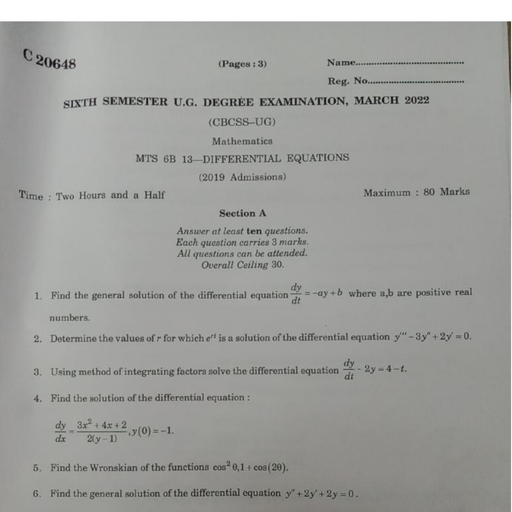
Page 1 : 1188, , Chapter 14 Multiple Integrals, , 14.6, , Triple Integrals, Triple Integrals Over a Rectangular Box, Just as the mass of a piece of straight, thin wire of linear mass density d(x), where, a  x  b, is given by the single integral 兰ab d(x) dx, and the mass of a thin plate D of, mass density s(x, y) is given by the double integral 兰兰D s(x, y) dA, we will now see, that the mass of a solid object T with mass density r(x, y, z) is given by a triple integral., Let’s consider the simplest case in which the solid takes the form of a rectangular, box:, B  [a, b]  [c, d]  [p, q]  {(x, y, z) 冟 a  x  b, c  y  d, p  z  q}, Suppose that the mass density of the solid is r(x, y, z) g/m3, where r is a positive continuous function defined on B. Let, , z, , a  x 0  x 1  p  x i1  x i  p  x l  b, , Bijk, , c  y0  y1  p  yj1  yj  p  ym  d, p  z 0  z 1  p  z k1  z k  p  z n  q, 0, y, x, , FIGURE 1, A partition P  {Bijk} of B, , be regular partitions of the intervals [a, b], [c, d], and [p, q] of length ⌬x  (b  a)>l,, ⌬y  (d  c)>m, and ⌬z  (q  p)>n, respectively. The planes x  x i, for 1  i  l,, y  yj, for 1  j  m, and z  z k, for 1  k  n, parallel to the yz-, xz-, and xycoordinate planes divide the box B into N  lmn boxes B111, B112, p , Bijk, p , Blmn,, as shown in Figure 1. The volume of Bijk is ⌬V  ⌬x ⌬y ⌬z., Let (x *, ijk, y *, ijk, z *, ijk) be an arbitrary point in Bijk. If l, m, and n are large (so that the, dimensions of Bijk are small), then the continuity of r implies that r(x, y, z) does not, vary appreciably from r(x *, ijk, y *, ijk, z *, ijk) , whenever (x, y, z) is in Bijk. Therefore, we can, approximate the mass of Bijk by, r(x *, ijk, y *, ijk, z *, ijk) ⌬V, , constant mass density ⴢ volume, , where ⌬V  ⌬x ⌬y ⌬z. Adding up the masses of the N boxes, we see that the mass of, the box B is approximately, l, , m, , n, , ijk, y *, ijk, z *, ijk) ⌬V, a a a r(x *, , (1), , i1 j1 k1, , We expect the approximation to improve as l, m, and n get larger and larger. Therefore, it is reasonable to define the mass of the box B as, l, , lim, , m, , n, , ijk, y *, ijk, z *, ijk) ⌬V, a a a r(x *, , l, m, n→⬁ i1 j1 k1, , (2), , The expression in (1) is an example of a Riemann sum of a function of three, variables over a box and the corresponding limit in (2) is the triple integral of f over, B. More generally, we have the following definitions. Notice that no assumption, regarding the sign of f(x, y, z) is made in these definitions.

Page 2 : 14.6 Triple Integrals, , 1189, , DEFINITION Triple Integral of f Over a Rectangular Box B, Let f be a continuous function of three variables defined on a rectangular box, B, and let P  {Bijk} be a partition of B., 1. A Riemann sum of f over B with respect to the partition P is a sum of the, form, l, , m, , n, , ijk, y *, ijk, z *, ijk) ⌬V, a a a f(x *, i1 j1 k1, , * , y*, where (x ijk, ijk, z *, ijk) is a point in Bijk., 2. The triple integral of f over B is, , 冮冮冮, , l, , f(x, y, z) dV , , B, , m, , n, , ijk, y *, ijk, z *, ijk) ⌬V, a a a f(x *, , lim, , l, m, n→⬁ i1 j1 k1, , if the limit exists for all choices of (x *, ijk, y *, ijk, z *, ijk) in Bijk., , As in the case of double integrals, a triple integral may be found by evaluating an, appropriate iterated integral., , THEOREM 1, Let f be continuous on the rectangular box, B  {(x, y, z) 冟 a  x  b, c  y  d, p  z  q}, Then, q, , d, , b, , 冮冮冮 f(x, y, z) dV  冮 冮 冮 f(x, y, z) dx dy dz, p, , B, , c, , (3), , a, , The iterated integral in Equation (3) is evaluated by first integrating with respect, to x while holding y and z constant, then integrating with respect to y while holding z, constant, and finally integrating with respect to z. The triple integral in Equation (3), can also be expressed as any one of five other iterated integrals, each with a different, order of integration. For example, we can write, , 冮冮冮, , b, , f(x, y, z) dV , , B, , q, , d, , 冮 冮 冮 f(x, y, z) dy dz dx, a, , p, , c, , where the iterated integral is evaluated by successively integrating with respect to y,, z, and then x. (Remember, we work “from the inside out.”), , EXAMPLE 1 Evaluate 兰兰兰B (x 2y, , yz 2) dV, where, , B  {(x, y, z) 冟 1  x  1, 0  y  3, 1  z  2}

Page 3 : 1190, , Chapter 14 Multiple Integrals, , Solution We can express the given integral as one of six integrals. For example, if, we choose to integrate with respect to x, y, and z, in that order, then we obtain, , 冮冮冮, , 2, , (x 2y, , yz 2) dV , , 冮冮冮, 1, , B, , 3, , 冮冮, , 3, , 2, , 3, , 1, , , , 0, , 冮冮, 1, , , , 0, , 冮, , 2, , 1, , (x 2y, , 1, c x 3y, 3, 2, c y, 3, , 冮 (3, , xyz 2 d, , x1, , dy dz, x1, , 2yz 2 d dy dz, , 1, c y2, 3, , 2, , , , yz 2) dx dy dz, , 1, , 0, , 2, , , , 1, , y 2z 2 d, , y3, , dz, y0, , 9z 2) dz  C3z, , 1, , 3z 3 D 1  24, 2, , Triple Integrals Over General Bounded Regions in Space, z, , T, , Bijk, , y, x, , We can extend the definition of the triple integral to more general regions using the same, technique that we used for double integrals. Suppose that T is a bounded solid region, in space. Then it can be enclosed in a rectangular box B  [a, b]  [c, d]  [p, q]., Let P be a regular partition of B into N  lmn boxes with sides of length, ⌬x  (b  a)>l, ⌬y  (d  c)>m, ⌬z  (q  p)>n, and volume ⌬V  ⌬x ⌬y ⌬z., Thus, P  {B111, B112, p , Bijk, p , Blmn}. (See Figure 2.), Define, F(x, y, z)  e, , f(x, y, z), 0, , if (x, y, z) is in T, if (x, y, z) is in B but not in T, , Then a Riemann sum of f over T with respect to the partition P is given by, , FIGURE 2, The box Bijk is a typical element of the, partition of B., , l, , m, , n, , ijk, y *, ijk, z *, ijk) ⌬V, a a a F(x *, i1 j1 k1, , where (x *, ijk, y *, ijk, z *, ijk) is an arbitrary point in Bijk and ⌬V is the volume of Bijk. If we take, the limit of these sums as l, m, n approach infinity, we obtain the triple integral of f, over T. Thus,, , 冮冮冮, T, , l, , f(x, y, z) dV , , lim, , m, , n, , ijk, y *, ijk, z *, ijk) ⌬V, a a a F(x *, , l, m, n→⬁ i1 j1 k1, , provided that the limit exists for all choices of (x *, ijk, y *, ijk, z *, ijk) in T., Notes, 1. If f is continuous and the surface bounding T is “sufficiently smooth,” it can be, shown that f is integrable over T., 2. The properties of double integrals that are listed in Theorem 1, Section 14.1, with, the necessary modifications are also enjoyed by triple integrals., , Evaluating Triple Integrals Over General Regions, We will now restrict our attention to certain types of regions. A region T is z-simple, if it lies between the graphs of two continuous functions of x and y, that is, if, T  {(x, y, z) 冟 (x, y) 僆 R, k 1 (x, y)  z  k 2(x, y)}

Page 4 : 14.6 Triple Integrals, , 1191, , where R is the projection of T onto the xy-plane. (See Figure 3.) If f is continuous on, T, then, , 冮冮冮, , 冮冮 冮, c, , f(x, y, z) dV , , T, , R, , k2(x, y), , (4), , f(x, y, z) dzd dA, , k1(x, y), , z, z  k 2 (x,y), , T, z  k 1 (x,y), a, , FIGURE 3, A z-simple region T is bounded by the, surfaces z  k 1 (x, y) and z  k 2(x, y)., , y, , y  t1 (x), , b, , R, , x, , y  t2 (x), , The iterated integral on the right-hand side of Equation (4) is evaluated by first integrating with respect to z while holding x and y constant. The resulting double integral, is then evaluated by using the method of Section 14.2. For example, if R is y-simple,, as shown in Figure 3, then, R  {(x, y) 冟 a  x  b, t1(x)  y  t2(x)}, in which case Equation (4) becomes, , 冮冮冮, , b, , f(x, y, z) dV , , 冮冮 冮, a, , T, , t2(x), , t1(x), , k2(x, y), , f(x, y, z) dz dy dx, , k1(x, y), , To determine the “limits of integration” with respect to z, notice that z runs from the, lower surface z  k 1 (x, y) to the upper surface z  k 2(x, y) as indicated by the arrow, in Figure 3., , EXAMPLE 2 Evaluate 兰兰兰T z dV where T is the solid in the first octant bounded by, the graphs of z  1  x 2 and y  x., Solution The solid T is shown in Figure 4a. The solid is z-simple because it is bounded, below by the graph of z  k 1 (x, y)  0 and above by z  k 2(x, y)  1  x 2., y, , z, z  1  x2, , 1, , (1, 1), , 1, y x, , T, 1, , R, , R, y, , x, , z 0, , y x, , (a) The solid T is z-simple., , FIGURE 4, , 0, , 1, , x, , (b) The projection of the solid T onto, R in the xy-plane is y-simple.

Page 5 : 1192, , Chapter 14 Multiple Integrals, , The projection of T onto the xy-plane is the set R that is sketched in Figure 4b., Regarding R as a y-simple region, we obtain, , 冮冮冮, , z dV , , T, , 冮冮 冮, c, , 1, , 冮冮, 0, , , , , , 1, 2, 1, 2, 1, 2, , 1, , x, , 0, , 0, , 0, , z dz dy dx, , 0, , 2, , 1 z1x, c z2d, dy dx, 2 z0, , 1, , x, , 冮 冮 (1  x ), , 2 2, , 0, , dy dx, , 0, , 1, , 冮 C (1  x ) yD, 2 2, , 0, , 冮, , 1x2, , x, , 冮冮冮, , z dzd dA , , zk1(x, y), , R, , , , zk2(x, y), , yx, y0, , dx, , 0, , 1, , 1, 1, 1 1, 1, x(1  x 2)2 dx  c a b a b a b (1  x 2)3 d , 2, 2 3, 12, 0, , There are two other simple regions besides the z-simple region just considered. An, x-simple region T is one that lies between the graphs of two continuous functions of, y and z. In other words, T may be described as, T  {(x, y, z) 冟 (y, z) 僆 R, k 1 (y, z)  x  k 2(y, z)}, where R is the projection of T onto the yz-plane. (See Figure 5.) Here, we have, , 冮冮冮, , f(x, y, z) dV , , T, , 冮冮 冮, c, , R, , k2(y, z), , f(x, y, z) dxd dA, , (5), , k1(y, z), , The (double) integral over the plane region R is evaluated by integrating with respect, to y or z first depending on whether R is y-simple or z-simple., z, , R, 0, y, x = k1(y, z), , T, , FIGURE 5, An x-simple region T is bounded by the, surfaces x  k 1 (y, z) and x  k 2(y, z) ., , x, x = k2(y, z), , A y-simple region T lies between the graphs of two continuous functions of x, and z. In other words, T may be described as, T  {(x, y, z) 冟 (x, z) 僆 R, k 1 (x, z)  y  k 2(x, z)}, where R is the projection of T onto the xz-plane. (See Figure 6.) In this case we have, , 冮冮冮, T, , f(x, y, z) dV , , 冮冮 冮, c, , R, , k2(x, z), , k1(x, z), , f(x, y, z) dyd dA, , (6)

Page 6 : 14.6 Triple Integrals, , 1193, , z, , y = k2(x, z), , R, T, y = k1(x, z), , 0, , FIGURE 6, A y-simple region T is bounded by the, surfaces y  k 1 (x, z) and y  k 2(x, z)., , y, x, , Again depending on whether R is an x-simple or z-simple plane region, the double integration is carried out first with respect to x or z., , EXAMPLE 3 Evaluate 兰兰兰T 2x 2, inder x, , 2, , z 2 dV, where T is the region bounded by the cylz  2 and y  0., , z  1 and the planes y, 2, , Solution The solid T is shown in Figure 7a. Although T can be viewed as an xsimple or z-simple region, it is easier to view it as a y-simple region. (Try It!) In this, case we see that T is bounded to the left by the graph of the function y  k 1(x, z)  0, and to the right by the graph of the function y  k 2 (x, z)  2  z. The projection of, T onto the xz-plane is the set R, which is sketched in Figure 7b. We have, , 冮冮冮, , 2x 2, , z 2 dV , , T, , 冮冮 冮, , k2(x, z), , 冮冮 冮, , 2z, , c, , R, , , , c, , R, , , , 2x 2, , 2x 2, , z 2 dyd dA, , 0, , 冮冮 c2x, , y2z, 2, , z 2 yd, , 冮冮 2x, , 2, , dA, y0, , R, , , , z 2 dyd dA, , k1(x, z), , z 2 (2  z) dA, , R, , z, , z, x2 + z2 = 1, , 1, , y=2–z, , R, , T, y, x, (a) The solid T is viewed as being y-simple., , FIGURE 7, , x2 + z2 = 1, , –1, , 1, , x, , –1, (b) The projection of the solid T onto R, in the xz-plane

Page 7 : 1194, , Chapter 14 Multiple Integrals, , Since R is a circular region, it is more convenient to use polar coordinates when integrating over R. So letting x  r cos u and z  r sin u, we have, , 冮冮, , 2p, , 2x 2, , z 2 (2  z) dA , , 1, , 冮 冮 r(2  r sin u) r dr du, 0, , R, , 0, , 2p, , , , 1, , 冮 冮 (2r, 0, , , , 冮, , 2p, ,  r 3 sin u) dr du, , 冮, , 2p, , r1, 2, 1, c r 3  r 4 sin ud, du, 3, 4, r0, , 0, , , , 2, , 0, , 0, , 2, 1, a  sin ub du, 3, 4, , 2, c u, 3, , 2p, 1, 4p, cos ud , 4, 3, 0, , Therefore,, , 冮冮冮 2x, , 2, , z 2 dV , , 4p, 3, , T, , Volume, Mass, Center of Mass, and Moments of Inertia, Before looking at other examples, let’s list some applications of triple integrals. Let, f(x, y, z)  1 for all points in a solid T. Then the triple integral of f over T gives the, volume V of T; that is,, V, , 冮冮冮 dV, , (7), , T, , We also have the following., , DEFINITIONS Mass, Center of Mass, and Moments of Inertia, for Solids in Space, Suppose that r(x, y, z) gives the mass density at the point (x, y, z) of a solid T., Then the mass m of T is, m, , 冮冮冮 r(x, y, z) dV, , (8), , T, , The moments of T about the three coordinate planes are, M yz , , 冮冮冮 xr(x, y, z) dV, , (9a), , 冮冮冮 yr(x, y, z) dV, , (9b), , 冮冮冮 zr(x, y, z) dV, , (9c), , T, , M xz , , T, , M xy , , T

Page 8 : 14.6 Triple Integrals, , 1195, , The center of mass of T is located at the point (x, y, z), where, x, , M yz, m, , y, , ,, , M xz, m, , ,, , z, , M xy, , (10), , m, , and the moments of inertia of T about the three coordinate axes are, Ix , , 冮冮冮 (y, , 2, , z 2)r(x, y, z) dV, , (11a), , 2, , z 2)r(x, y, z) dV, , (11b), , 2, , y 2)r(x, y, z) dV, , (11c), , T, , Iy , , 冮冮冮 (x, T, , Iz , , 冮冮冮 (x, T, , If the mass density is constant, then the center of mass of a solid is called the centroid of T., , EXAMPLE 4 Let T be the solid tetrahedron bounded by the plane x y z  1, and the three coordinate planes x  0, y  0, and z  0. Find the mass of T if the, mass density of T is directly proportional to the distance between a base of T and a, point on T., Solution The solid T is shown in Figure 8a. It is x-, y-, and z-simple. For example, it, can be viewed as being x-simple if you observe that it is bounded by the surface, x  k 1 (y, z)  0 and the surface x  k 2 (y, z)  1  y  z. (Solve the equation, x y z  1 for x.), z, , z, , 1, x 1y z, , 1, T, , R, , x 0, , z 1y, R, , 1, , y, , x 1, (a) The solid T viewed as an x-simple region, , FIGURE 8, , 1, , y, , (b) The projection of the solid T onto the, yz-plane viewed as a z-simple region, , The projection of T onto the yz-plane is the set R shown in Figure 8b. Observe that, the upper boundary of R lies along the line that is the intersection of x y z  1, and the plane x  0 and hence has equation y z  1 or z  1  y. If we take, the base of T as the face of the tetrahedron lying on the xy-plane (actually, by symmetry, any face will do), then the mass density function for T is r(x, y, z)  kz,

Page 9 : 1196, , Chapter 14 Multiple Integrals, , where k is the constant of proportionality. Using Equation (8), we see that the required, mass is, m, , 冮冮冮 r(x, y, z) dV  冮冮冮 kz dV, T, , T, , 1, , k, , 1y, , 冮冮 冮, 0, , 0, , 冮冮, 0, , k, , 冮, 冮, , 1, , 0, , k, , 1y, , 0, , 1, , 0, , z dx dz dy, , View T as x-simple., , 0, , 1, , k, , 1yz, , CzxD x0, , x1yz, , 1, , dz dy  k, , 冮冮, 0, , 1y, , [(1  y)z  z 2] dz dy, , View R as z-simple., , 0, , 1, 1 z1y, c (1  y)z 2  z 3 d, dy, 2, 3 z0, 1, 1, 1, 1, k, (1  y)3 dy  kc a b a b (1  y)4 d , 6, 6, 4, 24, 0, , EXAMPLE 5 Let T be the solid that is bounded by the parabolic cylinder y  x 2 and, , the planes z  0 and y z  1. Find the center of mass of T, given that it has uniform density r(x, y, z)  1., Solution The solid T is shown in Figure 9a. It is x-, y-, and z-simple. Let’s choose to, view it as being z-simple. (You are also encouraged to solve the problem by viewing, T as x-simple and y-simple.) In this case we see that T lies between the xy-plane, z  k 1 (x, y)  0 and the plane z  k 2(x, y)  1  y. The projection of T onto the, xy-plane is the region R shown in Figure 9b. As a first step toward finding the center, of mass of T, let’s find the mass of T. Using Equation (8), we have, m, , 冮冮冮 r(x, y, z) dV  冮冮冮 dV, T, , T, , 1, , , , 1, , 冮 冮冮, 1, , 2, , x, , 1, , , , , 1y, , dz dy dx , , 0, , 1, , 冮 冮 (1  y) dy dx  冮, 1, , 冮, , 1, , 1, , 1, , 2, , 冮 冮 CzD, 1, , 1, , x2, , 1, , 1, a  x2, 1 2, , x, , cy , , 1 2 y1, dx, y d, 2, yx2, 1 5 1, 8, x d , 10, 15, 1, , z 1, , T, , 1, R, , R, z 0, , y, , x, , FIGURE 9, , dy dx, , y, y, , y x, , z0, , 1 4, 1, 1, x b dx  c x  x 3, 2, 2, 3, , z, , 2, , z1y, , (a) The solid T is viewed as a, z-simple region., , 1, , y  x2, 1, , x, , (b) The projection R of T onto the, xy-plane viewed as being y-simple

Page 10 : 14.6 Triple Integrals, , 1197, , By symmetry we see that x ⫽ 0. Next, using Equations (9b) and (10), we have, y⫽, , 冮冮冮 yr(x, y, z) dV ⫽ 8 冮冮冮 y dV, , 1, m, , 15, , T, , ⫽, , T, , 1, , 1, , 冮 冮冮, , 15, 8, , ⫺1, , x2, , 1, , ⫽, , 15, 8, , 冮 冮, , 15, 8, , 1, , ⫽, , ⫺1, , 冮, , 1⫺y, , y dz dy dx ⫽, , 0, , 1, , x2, , 1, , 冮 冮 C yzD, ⫺1, , x2, , z⫽1⫺y, z⫽0, , dy dx, , 1, , y⫽1, 1, 1, c y2 ⫺ y3d, dx, 3, y⫽x2, ⫺1 2, , 冮, , 15, 8, , (y ⫺ y 2) dy dx ⫽, , 1, , 15, 8, , 1, 1, 1, 15, a ⫺ x 4 ⫹ x 6 b dx ⫽ 2a b, 2, 3, 8, ⫺1 6, , 1, , 冮 a6 ⫺ 2 x, 1, , 1, , 4, , ⫹, , 0, , 1 6, x b dx, 3, , The integrand is an even function., , 1, , 15 1, 1 5, 1 7, 3, ⫽, c x⫺, x ⫹, x d ⫽, 4 6, 10, 21, 7, 0, Similarly, you can verify that, z⫽, , 冮冮冮 zr(x, y, z) dV ⫽ 8 冮冮冮 z dV, , 1, m, , 15, , T, , ⫽, , 15, 8, , Use Equation (9c)., , T, , 1, , 1, , ⫺1, , 2, , 冮 冮冮, x, , 1⫺y, , 2, 7, , z dz dy dx ⫽, , 0, , Therefore, the center of mass of T is located at the point 1 0, 37, 27 2 ., z, , EXAMPLE 6 Find the moments of inertia about the three coordinate axes for the solid, rectangular parallelepiped of constant density k shown in Figure 10., , b, , Solution, , Using Equation (11a) with r(x, y, z) ⫽ k, we obtain, , 0, , c, , a, , Ix ⫽, , y, , x, , 冮冮冮 (y, , 2, , ⫹ z 2)k dV, , T, , FIGURE 10, The center of the solid is placed, at the origin., , ⫽, , c>2, , b>2, , a>2, , ⫺c>2, , ⫺b>2, , ⫺a>2, , 冮 冮 冮, , k(y 2 ⫹ z 2) dx dy dz, , Observe that the integrand is an even function of x, y, and z. Taking advantage of symmetry, we can write, c>2, , Ix ⫽ 8k, , b>2, , 冮 冮 冮, 0, , 0, , 冮 冮, 0, , ⫽ 4ka, , 冮, , c>2, , ⫽, , (y 2 ⫹ z 2) dy dz ⫽ 4ka, , a, , 冮, , c>2, , 0, , 3, , 冮 冮, 0, , b>2, , 0, , 0, , ⫽ 4kaa, , c>2, , (y 2 ⫹ z 2) dx dy dz ⫽ 8k, , 0, , c>2, , ⫽ 4ka, , a>2, , 2, , 0, , b>2, , C (y 2 ⫹ z 2)xD x⫽0 dy dz, , y⫽b>2, 1, c y 3 ⫹ z 2yd, dz, 3, y⫽0, , 3, , z⫽c>2, b, bz, b, b, ⫹, b dz ⫽ 4kaa z ⫹ z 3 b `, 24, 2, 24, 6, z⫽0, , b 3c, bc3, kabc 2, ⫹, b⫽, (b ⫹ c2), 48, 48, 12, , 1, m(b 2 ⫹ c2), 12, , m ⫽ kabc ⫽ mass of the solid, , x⫽a>2

Page 11 : 1198, , Chapter 14 Multiple Integrals, , Similarly, we find, Iy , , 14.6, , 1, m(a 2, 12, , c 2), , 14.6, , 1. f(x, y, z)  x y z; B  {(x, y, z) 冟 0  x  2, 0  y  1,, 0  z  3}. Integrate (a) with respect to x, y, and z, in that, order, and (b) with respect to z, y, and x, in that order., , 3. a. What is a z-simple region in space? An x-simple region?, A y-simple region?, b. Write the integral 兰兰兰T f(x, y, z) dV, where T is a zsimple region. An x-simple region. A y-simple region., , In Exercises 11–14, the figure shows the region of integration for, 兰兰兰T f(x, y, z) dV. Express the triple integral as an iterated integral in six different ways using different orders of integration., 11., , 3, , 3. f(x, y, z)  xy 2 yz 2; B  {(x, y, z) 冟 0  x  2,, 1  y  1, 0  z  3}. Integrate (a) with respect to z, y,, and x, in that order, and (b) with respect to x, y, and z, in, that order., , 4. f(x, y, z)  xy 2 cos z; B  5 (x, y, z) 冟 0  x  2, 0  y  3,, 0  z  p2 6 . Integrate (a) with respect to y, z, and x, in that, order, and (b) with respect to y, x, and z, in that order., , 冮冮冮, 0, , 7., , 0, , p>2, , 2, , 2, , 24z2, , 1, , 0, , 0, , 4, , 1, , x, , 0, , 0, , e, , 10., , x, , 1, , 1, , y 2z dx dz dy, 2 1y ex dz dx dy, 2, , 1>(xy), , 0, , 0, , 2 ln y dz dy dx, , 2, , 2, , y, , x2, , z2  4, y 3, , 3, , y, , x, , 14., , z, , z, z 1, , x, , y, , z 1, , x  y2, , 2xz dx dy dz, , z  x2, , 0, , 1, , 0, , 冮冮冮, , 冮冮冮, , z, , 4z  12, , 4, , 13., , y cos x dy dz dx, , 0, , 冮 冮冮, , z, , 3y, , x, , 11z, , 1, , 冮冮冮, , 6., , 0, , 冮 冮冮, 1, , 9., , 1, , x dz dy dx, , 0, , 0, , 8., , y, , 6x, , 2, , In Exercises 5–10, evaluate the iterated integral., x, , 12., , z, , 2. f(x, y, z)  xyz; B  {(x, y, z) 冟 1  x  1, 0  y  2,, 2  z  6}. Integrate (a) with respect to y, x, and z, in, that order, and (b) with respect to x, z, and y, in that order., , 5., , b 2), , EXERCISES, , In Exercises 1–4, evaluate the integral 兰兰兰B f(x, y, z) dV using, the indicated order of integration., , x, , 1, m(a 2, 12, , CONCEPT QUESTIONS, , 1. a. Define the Riemann sum of f over a rectangular box B., b. Define the triple integral of f over B., 2. Suppose that f is continuous on the rectangular box, B  [a, b]  [c, d]  [p, q]., a. Explain how you would evaluate 兰兰兰B f(x, y, z) dV., b. Write all iterated integrals that are associated with the, triple integral of part (a)., , 1, , Iz , , and, , x, , y, , y2, , y, x, , In Exercises 15–22, evaluate the integral 兰兰兰T f(x, y, z) dV., 15. f(x, y, z)  x; T is the tetrahedron bounded by the planes, x  0, y  0, z  0, and x y z  1, 16. f(x, y, z)  y; T is the region bounded by the planes x  0,, y  0, z  0, and 2x 3y z  6, 17. f(x, y, z)  2z; T is the region bounded by the cylinder, y  x 3 and the planes y  x, z  2x, and z  0, , V Videos for selected exercises are available online at www.academic.cengage.com/login.

Page 12 : 14.6 Triple Integrals, 18. f(x, y, z)  x 2y; T is the region bounded by the cylinder y  1x and the planes y  x, z  2x, and z  0, 19. f(x, y, z)  y; T is the region bounded by the paraboloid, y  x 2 z 2 and the plane y  4, 20. f(x, y, z)  z; T is the region bounded by the parabolic, cylinder y  x 2 and the planes y z  1 and z  0, 21. f(x, y, z)  z; T is the region bounded by the cylinder, x 2 z 2  4 and the planes x  2y, y  0, and z  0, 22. f(x, y, z)  2x 2 z 2; T is the region bounded by the, paraboloids y  x 2 z 2 and y  8  x 2  z 2, , 1199, , of the subrectangles Rijk(1  i, j, k  2) to estimate, 兰兰兰B f(x, y, z) dV., b. Find the exact value of 兰兰兰B f(x, y, z) dV., 40. Let f(x, y, z)  2x 2 y 2 z 2 and let, B  {(x, y, z) 冟 0  x  4, 0  y  2, 0  z  1}., a. Use a Riemann sum with m  n  p  2, and choose, the evaluation point (x *, ijk, y *, ijk, z *, ijk) to be the midpoint, of the subrectangles Rijk(1  i, j, k  2) to estimate, 兰兰兰B f(x, y, z) dV., cas b. Use a computer algebra system to estimate, 兰兰兰B f(x, y, z) dV accurate to four decimal places., , In Exercises 23–28, sketch the solid bounded by the graphs of, the equations, and then use a triple integral to find the volume of cas In Exercises 41 and 42, use a computer algebra system to estithe solid., mate the triple integral accurate to four decimal places., 23. 3x, , z  6, x  0, y  0, z  0, , 2y, , 24. y  2z,, , 1, , 41., , y  x , y  4, z  0, 2, , 25. x  4  y 2, x, , z  4, x  0, z  0, , y2, , 42., , In Exercises 31–34, sketch the solid whose volume is given by, the iterated integral., 1, , 1y, , 0, , 0, , 1, , dz dx dy, , 32., , 0, , 冮冮 冮, 2 0, , 0, , y, , 2, , 0, , 1, , dz dx dy, , 34., , 1y, , 冮冮 冮, 0, , 4y2, , 2, , 33., , 1xy, , cos xy, 21, , 1, , dx dy dz, , 1x2, , 1x, , 0, , xyz 2, , xeyz dz dy dx, , 0, , In Exercises 43–46, find the center of mass of the solid T having, the given mass density., , z2  4, , 30. Find the volume of the tetrahedron with vertices (0, 0, 0) ,, (1, 0, 0) , (1, 0, 1) , and (1, 1, 0) ., , 冮冮 冮, , 2, , 冮冮 冮, 0, , 29. Find the volume of the tetrahedron with vertices (0, 0, 0),, (1, 0, 0), (0, 3, 0), and (0, 0, 2) ., , 31., , 0, , 1, , y 2, z  8  x 2  y 2, , z 2  4,, , 28. x 2, , 冮 冮冮, 1, , 26. z  1  x 2, y  x, y  2  x, z  0, 27. z  x 2, , 2, , 冮冮, 0, , 22z, , dx dz dy, , 0, , 11y, , 11y, , 冮, , y, , dz dx dy, , 0, , In Exercises 35–38, express the triple integral 兰兰兰T f(x, y, z) dV, as an iterated integral in six different ways using different orders, of integration., 35. T is the solid bounded by the planes x, x  0, y  0, and z  0., , 2y, , 3z  6,, , 36. T is the tetrahedron bounded by the planes z  0, x  0,, y  0, y  2  2z, and z  1  x., 37. T is the solid bounded by the circular cylinder x 2, and the planes z  0 and z  2., , y2  1, , 38. T is the solid bounded by the parabolic cylinder y  x and, the planes z  0 and z  4  y., 2, , 39. Let f(x, y, z)  x y z and let B  {(x, y, z) 冟 0  x  4,, 0  y  4, 0  z  4}., a. Use a Riemann sum with m  n  p  2, and choose, the evaluation point (x *, ijk, y *, ijk, z *, ijk) to be the midpoint, , 43. T is the tetrahedron bounded by the planes x  0, y  0,, z  0, and x y z  1. The mass density at a point P of, T is directly proportional to the distance between P and the, yz-plane., 44. T is the wedge bounded by the planes x  0, y  0, z  0,, z  23 y 2 and x  1. The mass density at a point P of, T is directly proportional to the distance between P and the, xy-plane., 45. T is the solid bounded by the cylinder y 2 z 2  4 and the, planes x  0 and x  3. The mass density at a point P of T, is directly proportional to the distance between P and the, yz-plane., 46. T is the solid bounded by the parabolic cylinder z  1  x 2, and the planes y z  1, y  0, and z  0. T has uniform, mass density r(x, y, z)  k, where k is a constant., In Exercises 47–50, set up, but do not evaluate, the iterated integral giving the mass of the solid T having mass density given by, the function r., 47. T is the solid bounded by the cylinder x 2 z 2  1 in the, first octant and the plane z y  1; r(x, y, z)  xy z 2, 48. T is the solid bounded by the ellipsoid, 36x 2 9y 2 4z 2  36 and the planes y  0, and z  0; r(x, y, z)  1yz, 49. T is the solid bounded by the parabolic cylinder z  1  y 2, and the planes 2x y  2, y  0, and z  0;, r(x, y, z)  2x 2 y 2 z 2

Page 13 : 1200, , Chapter 14 Multiple Integrals, , 50. T is the upper hemisphere bounded by the sphere, x 2 y 2 z 2  1 and the plane z  0;, r(x, y, z)  21 x 2 y 2, , 56. Find the average value of f(x, y, z)  x 2, tetrahedron bounded by the planes x y, y  0, and z  0., , 51. Let T be a cube bounded by the planes x  0, x  1, y  0,, y  1, z  0, and z  1. Find the moments of inertia of T, with respect to the coordinate axes if T has constant mass, density k., , 57. Find the average value of f(x, y, z)  xyz over the solid, region lying inside the spherical ball of radius 2 with center, at the origin and in the first octant., 58. Average Temperature in a Room A rectangular room can be, described by the set B  {(x, y, z) 冟 0  x  20,, 0  y  40, 0  z  9}. If the temperature (in degrees, Fahrenheit) at a point (x, y, z) in the room is given by, f(x, y, z)  60 0.2x 0.1y 0.2z, what is the average, temperature in the room?, , 52. Let T be a rectangular box bounded by the planes x  0,, x  a, y  0, y  b, z  0, and z  c. Find the moments of, inertia of T with respect to the coordinate axes if T has constant mass density k., 53. Let T be the solid bounded by the planes x y z  1,, x  0, y  0, and z  0. Find the moments of inertia of T, with respect to the x-, y-, and z-axes if T has mass density, given by r(x, y, z)  x., , 59. Find the region T that will make the value of, 2, 2, 2 1>3, 兰兰兰T (1  2x  3y  z ) dV as large as possible., 60. Find the values of a and b that will maximize, 2, 2, 2, 兰兰兰T (4  x  y  z ) dV, where, T  {(x, y, z) 冟 1  a  x 2 y 2 z 2  b  2}., , 54. Let T be the solid bounded by the cylinder y  x and the, planes y  x, z  0, and z  x. Find the moments of inertia, of T with respect to the coordinate axes if T has mass density given by r(x, y, z)  z., 2, , In Exercises 61–64, determine whether the statement is true or, false. If it is true, explain why. If it is false, explain why or give, an example that shows it is false., , The average value of a function f of three variables over a solid, region T is defined to be, 1, fav , V(T), , 61. If B  [1, 1]  [2, 2]  [3, 3], then, 2, y 2 z 2 dV 0., 兰兰兰B 2x, , 冮冮冮 f(x, y, z) dV, , 62. If T is a solid sphere of radius a centered at the origin, then, 兰兰兰T x dV  0., , T, , where V(T) is the volume of T. Use this definition in Exercises, 55–58., , 2, , 63. 12 , 64., , 3, , 4, , 冮 冮 冮 21, 1, , 55. Find the average value of f(x, y, z)  x y z over the, rectangular box T bounded by the planes x  0, x  1,, y  0, y  2, z  0, and z  3., , 14.7, , y 2 z 2 over the, z  1, x  0,, , 1, , x2, , y2, , z 2 dz dy dx  6130, , 1, , 冮冮冮 k dV , , 28pk, , where, 3, , T, , T  {(x, y, z) 冟 1  (x  1)2, and k is a constant, , (y  2)2, , (z, , 1)2  4}, , Triple Integrals in Cylindrical and Spherical Coordinates, Just as some double integrals are easier to evaluate by using polar coordinates, we will, see that some triple integrals are easier to evaluate by using cylindrical or spherical, coordinates., , Cylindrical Coordinates, Let T be a z-simple region described by, T  {(x, y, z) 冟 (x, y) 僆 R, h 1 (x, y)  z  h 2(x, y)}, where R is the projection of T onto the xy-plane. (See Figure 1.) As we saw in Section, 14.6, if f is continuous on T, then, , 冮冮冮, T, , f(x, y, z) dV , , 冮冮 冮, c, , R, , h2(x, y), , h1(x, y), , f(x, y, z) dzd dA, , (1)

Page 14 : 14.7, , Triple Integrals in Cylindrical and Spherical Coordinates, , 1201, , z, z = h2(x, y), , T, , z = h1(x, y), 0, r = t1(¨), , R, , ¨=b, r = t2(¨), , x, , FIGURE 1, T viewed as a z-simple region, , ¨=a, , y, , Now suppose that the region R can be described in polar coordinates by, R  {(r, u) 冟 a  u  b, t1(u)  r  t2(u)}, Then, since x  r cos u, y  r sin u, and z  z in cylindrical coordinates, we use Equation (2) in Section 14.3 to obtain the following formula., Triple Integral in Cylindrical Coordinates, , 冮冮冮, , b, , f(x, y, z) dV , , 冮冮 冮, a, , T, , t 2(u), , t 1(u), , h2(r cos u, r sin u), , f(r cos u, r sin u, z) r dz dr du (2), , h1(r cos u, r sin u), , Note As an aid to remembering Equation (2), observe that the element of volume in, cylindrical coordinates is dV  r dz dr du, as is suggested by Figure 2., z, r d¨, , dz, , dr, , d¨, r, , FIGURE 2, The element of volume in cylindrical, coordinates is dV  r dz dr du., , y, , x, , EXAMPLE 1 A solid T is bounded by the cone z  2x 2, , y 2 and the plane z  2., (See Figure 3.) The mass density at any point of the solid is proportional to the distance between the axis of the cone and the point. Find the mass of T., Solution, , The solid T is described by, , T  5 (x, y, z) 冟 (x, y) 僆 R, 2x 2, , y2  z  2 6

Page 15 : 1202, , Chapter 14 Multiple Integrals, , where R  {(x, y) 冟 0  x 2, , z, , y 2  4}. In cylindrical coordinates,, , T  {(r, u, z) 冟 0  u  2p, 0  r  2, r  z  2}, and, T, , R, x, , R  {(r, u) 冟 0  u  2p, 0  r  2}, , z=2, , Since the density of the solid at (x, y, z) is proportional to the distance from the z-axis, to the point in question, we see that the density function is, , y, 2, , r(x, y, z)  k2x 2, , 2, , x +y =4, , y 2  kr, , where k is the constant of proportionality. Therefore, if we use Equation (8) in Section 14.6, the mass of T is, , FIGURE 3, The arrow runs from the lower surface, z  h 1 (x, y)  2x 2 y 2 to the, upper surface z  h 2(x, y)  2 of T., , m, , 冮冮冮 r(x, y, z) dV  冮冮冮 k2x, T, , 2, , 冮 冮冮, 0, , 0, , (kr) r dz dr du, , 2, , 冮 冮 Cr zD, 2, , 0, , k, , 2, , r, , 2p, , k, , y 2 dV, , T, , 2p, , , , 2, , 0, , 2p, , 冮, , 0, , 2p, , z2, , dr du  k, , zr, , 2, , 冮 冮 (2r, 0, , 2, ,  r 3) dr du, , 0, , r2, 2, 1, 4, c r 3  r 4d, du  k, 3, 4, 3, r0, , 冮, , 2p, , du , , 0, , 8, pk, 3, , EXAMPLE 2 Find the centroid of a homogeneous solid hemisphere of radius a., z, , z = √a2 – x2 – y2, , a, , where, , T, , a, , R, , The solid T is shown in Figure 4. In rectangular coordinates we can write, T  5 (x, y, z) 冟 (x, y) 僆 R, 0  z  2a 2  x 2  y 2 6, R  {(x, y) 冟 0  x 2, , y 2  a 2}, , In cylindrical coordinates we have, , a, y, 2, , x, , Solution, , 2, , x +y =a, , 2, , FIGURE 4, A homogeneous solid hemisphere of, radius a, , and, , T  5 (r, u, z) 冟 0  u  2p, 0  r  a, 0  z  2a 2  r 2 6, R  {(r, u) 冟 0  u  2p, 0  r  a}, , By symmetry the centroid lies on the z-axis. Therefore, it suffices to find z  M xy>V,, where V, the volume of T, is 12 ⴢ 43 pa 3, or 23 pa 3. Using Equation (9c) in Section 14.6,, with r(x, y, z)  1, we obtain, 2p, , M xy , , 冮冮冮 z dV  冮 冮 冮, 0, , T, , 2p, , , , 冮 冮, 0, , , , a, , 1, 2, , a, , 0, , 冮, , 0, , 2p, , 0, , 2, , 1 z2a, c z2d, 2 z0, , 2a2 r2, , z r dz dr du, , 0, , r2, , r dr du , , 1, 2, , 2p, , a, , 冮 冮 (a, 0, , 2, ,  r 2) r dr du, , 0, , ra, , 1, 1, c a 2r 2  r 4 d, du, 2, 4, r0, , 1 1,  a a4b, 2 4, , 冮, , 0, , 2p, , du , , 1 4, 1, a (2p)  pa 4, 8, 4, , Copyright 2009 Cengage Learning. All Rights Reserved. May not be copied, scanned, or duplicated, in whole or in part.

Page 16 : 14.7, , Triple Integrals in Cylindrical and Spherical Coordinates, , 1203, , Therefore,, z, , M xy, V, , , , pa 4, 3, 3, ⴢ,  a, 4, 8, 2pa 3, , so the centroid is located at the point 1 0, 0, 3a8 2 ., , Spherical Coordinates, When the region of integration is bounded by portions of spheres and cones, a triple, integral is generally easier to evaluate if it is expressed in terms of spherical coordinates. Recall from Section 11.7 that the relationship between spherical coordinates, r, f, u and rectangular coordinates x, y, z is given by, x  r sin f cos u,, z, , ®, , z  r cos f, , (3), , (See Figure 5.), To see the role played by spherical coordinates in integration, let’s consider the, simplest case in which the region of integration is a spherical wedge (the analog of a, rectangular box), , P( ®, ƒ, ¨ ), or P(x, y, z), , ƒ, , T  {(r, f, u) 冟 a  r  b, c  f  d, a  u  b}, , O, ¨, , y  r sin f sin u,, , y, , x, , FIGURE 5, The point P has representation (r, f, u), in spherical coordinates and (x, y, z) in, rectangular coordinates., , where a  0, 0  d  c  p, and 0  b  a  2p. To integrate over such a region,, let, a  r0  r1  p  ri1  ri  p  rl  b, c  f0  f1  p  fj1  fj  p  fm  d, a  u0  u1  p  uk1  uk  p  un  b, be regular partitions of the intervals [a, b], [c, d], and [a, b], respectively, where, ⌬r  (b  a)>l, ⌬f  (d  c)>m and ⌬u  (b  a)>n. The concentric spheres ri,, where 1  i  l, half-cones f  fj, where 1  j  m, and the half-planes u  uk,, where 1  k  n, divide the spherical wedge T into N  lmn spherical wedges, T111, T112, p , Tlmn. A typical wedge Tijk comprising the spherical partition P  {Tijk} is, shown in Figure 6., z, , ® = ® i+1, , ƒ = ƒj, , ® = ®i, , ƒ = ƒj+1, Δƒ, , Δ®, ® i Δƒ, , FIGURE 6, A typical spherical wedge in, the partition P of the solid T, , Δ¨, x, , r i  ® i sin ƒj, , y, ¨ = ¨k+1, ® i sin ƒj D ¨, ¨ = ¨k, , If you refer to Figure 6, you will see that Tijk is approximately a rectangular box, with dimensions ⌬r, ri ⌬f (the arc of a circle with radius ri that subtends an angle of

Page 17 : 1204, , Chapter 14 Multiple Integrals, , ⌬f) and ri sin fj ⌬u (the arc of a circle with radius ri sin fj and subtending an angle, of ⌬u). Thus, its volume ⌬V is, ⌬V  r2i sin fj ⌬r ⌬f ⌬u, Therefore, an approximation to a Riemann sum of f over T is, l, , m, , n, , 2, i sin f*, i sin f*, j cos u*, k , r*, i sin f*, j sin u*, k , r*, i cos f*, j )r*, j ⌬r ⌬f ⌬u, a a a f(r*, i1 j1 k1, , But this is a Riemann sum of the function, F(r, f, u)  f(r sin f cos u, r sin f sin u, r cos f)r2 sin f, and its limit is the triple integral, d, , b, , 冮冮冮, a, , c, , b, , F(r, f, u) r2 sin f dr df du, , a, , Therefore, we have the following formula for transforming a triple integral in rectangular coordinates into one involving spherical coordinates., , Triple Integral in Spherical Coordinates, , 冮冮冮, , d, , b, , f(x, y, z) dV , , T, , 冮冮冮, a, , c, , b, , f(r sin f cos u, r sin f sin u, r cos f)r2 sin f dr df du, , (4), , a, , where T is the spherical wedge, T  {(r, f, u) 冟 a  r  b, c  f  d, a  u  b}, , Equation (4) states that to transform a triple integral in rectangular coordinates to, one in spherical coordinates, make the substitutions, x  r sin f cos u,, , y  r sin f sin u,, , z  r cos f,, , and, , x2, , y2, , z 2  r2, , then make the appropriate change in the limits of integration, and replace dV by, r2 sin f dr df du. This element of volume can be recalled with the help of Figure 7., z, , d®, ® sin ƒ d¨, ®r, ƒ, , dƒ, , Δ®, ® dƒ, , FIGURE 7, The element of volume in spherical, coordinates is dV  r2 sin f dr df du., , ¨, x, , d¨, , y

Page 18 : 14.7, z, , Triple Integrals in Cylindrical and Spherical Coordinates, , 1205, , Equation (4) can be extended to include more general regions. For example, if T is, R-simple, that is, if the region T can be described by, , ®  h 2(ƒ, ¨), , T  {(r, f, u) 冟 h 1 (f, u)  r  h 2 (f, u), c  f  d, a  u  b}, then, ®  h 1(ƒ, ¨), , 冮冮冮 f(x, y, z) dV, , 0, , T, , y, , d, , b, , x, , , , FIGURE 8, A r-simple region is bounded by, the surfaces r  h 1 (f, u) and, r  h 2 (f, u), , 冮冮冮, c, , a, , h2(f, u), , f(r sin f cos u, r sin f sin u, r cos f)r2 sin f dr df du, , (5), , h1(f, u), , Observe that r-simple regions are precisely those regions that lie between two surfaces, r  h 1(f, u) and r  h 2(f, u), as shown in Figure 8. To find the limits of integration, with respect to r, we draw a radial line emanating from the origin. The line first intersects the surface, r  h 1(f, u), giving the lower limit of integration, and then intersects the surface r  h 2(f, u) , giving the upper limit of integration., , z, , EXAMPLE 3 Evaluate 兰兰兰T x dV, where T is the part of the region in the first octant, , T, , lying inside the sphere x 2, , y2 z2  1, ® 1, , x2, or, , T  5 (r, f, u) 冟 0  r  1, 0  f  p2 , 0  u  p2 6, , x, , Furthermore, x  r sin f cos u. Therefore, using Equation (4), we obtain, p>2, , 0, , T, , 0, , 冮 冮 冮 r sin, 3, , 0, , 冮 冮, 0, , ®  cos ƒ, , , , 1, 8, , p>2, , 0, , p>2, , 冮 冮, , p, 16, , 0, , 2, , f cos u dr df du, , 0, , p>2, , , , 1, , p>2, , 0, , , , (r sin f cos u)r2 sin f dr df du, , 0, , p>2, , T, , 1, , p>2, , 冮冮冮 x dV  冮 冮 冮, , , z, , z 2  1., , Solution The solid T is shown in Figure 9. Since the boundary of T is part of a sphere,, let’s use spherical coordinates. In terms of spherical coordinates we can write, , y, , FIGURE 9, T is the part of the ball, x 2 y 2 z 2  1 lying in the first, octant., , y2, , p>2, , (1  cos 2f)cos u df du , , 0, , 冮, , p>2, , p>2, , cos u du , , 0, , p>2, , r1, 1, 1, c r4 sin2 f cos ud, df du , 4, 4, r0, , p, sin u `, 16, 0, , , , 1, 8, , 冮, , 冮 冮, 0, , p>2, , sin2 f cos u df du, , 0, , 0, , p>2, , cos ucf , , fp>2, 1, sin 2fd, du, 2, f0, , p, 16, , π, __, 4, , EXAMPLE 4 Find the center of mass of the solid T of uniform density bounded by, y, x, , FIGURE 10, The solid T is bounded below, by part of a cone and above, by part of a sphere., , the cone z  2x 2, , y 2 and the sphere x 2, , y2, , z 2  z. (See Figure 10.), , Solution We first express the given equations in terms of spherical coordinates. The, equation of the cone is, r cos f  2r2 sin2 f cos2 u, , r2 sin2 f sin2u  r sin f

Page 20 : 14.7, , 14.7, , 3, , 1., , 冮 冮冮, 0, , 2p, , 2., , 0, 2, , 冮 冮冮, 0, , r dz dr du, , 0, 2r, , r dz dr du, , 0, p>2, , 2, , 冮 冮 冮r, , 2, , 0, , 0, , 2 sec f, , p>4, , 冮 冮 冮, 0, , sin f dr df du, , 0, , 2p, , 4., , r2, , 1, , 2p, , 3., , 0, , 1207, , EXERCISES, , In Exercises 1–4, sketch the solid whose volume is given by the, integral, and evaluate the integral., p>2, , Triple Integrals in Cylindrical and Spherical Coordinates, , r2 sin f dr df du, , 0, , In Exercises 5–18, solve the problem using cylindrical coordinates., 5. Evaluate 兰兰兰T 2x 2 y 2 dV, where T is the solid bounded, by the cylinder x 2 y 2  1 and the planes z  1 and, z  3., 2, , 2, , 6. Evaluate 兰兰兰T ex y dV, where T is the solid bounded by the, cylinder x 2 y 2  4 and the planes z  0 and z  4., , 17. Find the moment of inertia about the z-axis of a homogeneous solid bounded by the cone z  2x 2 y 2 and the, paraboloid z  x 2 y 2., 18. Find the moment of inertia about the z-axis of a solid, bounded by the cylinder x 2 y 2  4 and the planes z  0, and z  3 if the mass density at any point on the solid is, directly proportional to its distance from the xy-plane., In Exercises 19–24, solve the problem by using spherical, coordinates., 19. Evaluate 兰兰兰B 2x 2, x 2 y 2 z 2  1., 2, , y2, 2, , z 2 dV, where B is the unit ball, , 2 3>2, , 20. Evaluate 兰兰兰B e(x y z ) dV, where B is the part of the unit, ball x 2 y 2 z 2  1 lying in the first octant., 21. Evaluate 兰兰兰T y dV, where T is the solid bounded by the, hemisphere z  21  x 2  y 2 and the xy-plane., 22. Evaluate 兰兰兰T x 2 dV, where T is the part of the unit ball, x 2 y 2 z 2  1 lying in the first octant., , 7. Evaluate 兰兰兰T y dV, where T is the part of the solid in the, first octant lying inside the paraboloid z  4  x 2  y 2., , 23. Evaluate 兰兰兰T xz dV, where T is the solid bounded above by, the sphere x 2 y 2 z 2  4 and below by the cone, , 8. Evaluate 兰兰兰T x dV, where T is the part of the solid in the, first octant bounded by the paraboloid z  x 2 y 2 and the, plane z  4., , 24. Evaluate 兰兰兰T z dV, where T is the solid bounded above by, the sphere x 2 y 2 z 2  4 and below by the cone, , 9. Evaluate 兰兰兰T (x 2 y 2) dV, where T is the solid bounded, by the cone z  4  2x 2 y 2 and the xy-plane., 2, , 10. Evaluate 兰兰兰T y dV, where T is the solid that lies within, the cylinder x 2 y 2  1 and between the xy-plane and the, paraboloid z  2x 2 2y 2., 11. Find the volume of the solid bounded above by the sphere, x 2 y 2 z 2  9 and below by the paraboloid, 8z  x 2 y 2., 12. Find the volume of the solid bounded by the paraboloids, z  x 2 y 2 and z  12  2x 2  2y 2., 13. A solid is bounded by the cylinder x 2 y 2  4 and the, planes z  0 and z  3. Find the center of mass of the solid, if the mass density at any point is directly proportional to its, distance from the xy-plane., , z  2x 2, , z  2x 2, , y 2., , y 2., , 25. Find the volume of the solid that is bounded above by the, plane z  1 and below by the cone z  2x 2 y 2., 26. Find the volume of the solid bounded by the cone, z  2x 2 y 2, the cylinder x 2 y 2  4, and the plane, z  0., 27. Find the volume of the solid lying outside the cone, z  2x 2 y 2 and inside the upper hemisphere, x 2 y 2 z 2  1., 28. Find the volume of the solid lying above the cone f  p>6, and below the sphere r  4 cos f., 29. Find the centroid of a homogeneous solid hemisphere of, radius a., , 14. A solid is bounded by the cone z  2x 2 y 2 and the, plane z  4. Find its center of mass if the mass density at, P(x, y, z) is directly proportional to the distance between P, and the z-axis., , 30. Find the centroid of the solid of Exercise 28., , 15. Find the center of mass of a homogeneous solid bounded by, the paraboloid z  4  x 2  y 2 and z  0., , 32. Find the center of mass of the solid of Exercise 31., , 16. Find the center of mass of a homogeneous solid bounded by, the paraboloids z  x 2 y 2 and z  36  3x 2  3y 2., , 31. Find the mass of a solid hemisphere of radius a if the mass, density at any point on the solid is directly proportional to, its distance from the base of the solid., 33. Find the mass of the solid bounded by the cone, z  2x 2 y 2 and the plane z  2 if the mass density at, any point on the solid is directly proportional to the square, of its distance from the origin., , V Videos for selected exercises are available online at www.academic.cengage.com/login.

Page 21 : 1208, , Chapter 14 Multiple Integrals, , 34. Find the center of mass of the solid of Exercise 33., , 1, , 21x2, , 1, , 21x2, , 冮 冮, , 冮, , 2x2 y2, , (x 2, , y 2)3>2 dz dy dx, , 35. Find the moment of inertia about the z-axis of the solid of, Exercise 28, assuming that it has constant mass density., , 42., , 36. Find the moment of inertia with respect to the axis of symmetry for a solid hemisphere of radius a if the density at a, point is directly proportional to its distance from the center, of the base., , In Exercises 43 and 44, evaluate the integral by using spherical, coordinates., , 冮冮, , 43., , 0, , 37. Find the moment of inertia with respect to a diameter of the, base of a homogeneous solid hemisphere of radius a., 38. Show that the average distance from the center of a circle of, radius a to other points of the circle is 2a>3 and that the, average distance from the center of a sphere of radius a to, other points of the sphere is 3a>4., 39. Let T be a uniform solid of mass m bounded by the spheres, r  a and r  b, where 0  a  b. Show that the moment, of inertia of T about a diameter of T is, 2m b  a, a, b, 5 b 3  a3, 5, , I, , 5, , 40. a. Use the result of Exercise 39 to find the moment of inertia of a uniform solid ball of mass m and radius b about, a diameter of the ball., b. Use the result of Exercise 39 to find the moment of inertia of a hollow spherical shell of mass m and radius b, about a diameter of the shell., Hint: Find lim a→b I., , , In Exercises 41 and 42, evaluate the integral by using cylindrical, coordinates., 1, , 41., , 冮 冮, 1, , 21x2, , 0, , 14.8, , 冮, , 24x2 y2, , z dz dy dx, , 21x2, , 1, , y2, , 22x2 y2, , (x 2, , 2x2, , 0, , 3, , 29x2, , 3, , 29x2, , 冮 冮, , 44., , 冮, , 2x2, , 冮, , y2, , z 2)3>2 dz dy dx, , y2, 225x2 y2, , (x 2, , y2, , z 2)1>2 dz dy dx, , 4, , 45. The temperature (in degrees Fahrenheit) at a point (x, y, z), of a solid ball of radius 3 in. centered at the origin is given, by T(x, y, z)  20(x 2 y 2 z 2). What is the average temperature of the ball?, In Exercises 46–50, determine whether the statement is true or, false. If it is true, explain why. If it is false, explain why or give, an example that shows it is false., 46. The volume of the solid bounded above by the paraboloid, z  4  x 2  y 2 and below by the xy-plane in cylindrical, 2, coordinates is 兰02p 兰02 兰04r dz dr du., 47. 兰0p>2 兰02p 兰02 r2 sin f dr du df  16p, 3, 冟, 48. If T  5 (r, f, u) a  r  b, 0  f  p2 , 0  u  p2 6 , then, p, 3, 3, 兰兰兰T dV  6 (b  a )., 49. If T is a solid with constant density k, then its moment of, inertia about the z-axis is given by Iz  k 兰兰兰T r2 sin2 f dV., 50. If T  5 (r, f, u) 冟 0  r  a, 0  f  p2 , 0  u  2p 6 ,, then 兰兰兰T r cos u dV  0., , 0, , Change of Variables in Multiple Integrals, We often use a change of variable (a substitution) when we integrate a function of one, variable to transform the given integral into one that is easier to evaluate. For example, using the substitution x  sin u, we find, , 冮, , 1, , 21  x 2 dx , , 0, , 冮, , p>2, , cos2 u du , , 0, , , , 1, 2, , 冮, , p>2, , (1, , cos 2u) du, , 0, , p, 4, , Observe that the interval of integration is [0, 1] if we integrate with respect to x, and, it changes to C0, p2 D if we integrate with respect to u. More generally, the substitution, x  t(u) [so dx  t¿(u) du] enables us to write, , 冮, , b, , a, , where a  t(c) and b  t(d)., , d, , f(x) dx , , 冮 f(t(u))t¿(u) du, c, , (1)

Page 22 : 14.8, , Change of Variables in Multiple Integrals, , 1209, , As you have also seen on many occasions, a change of variables can be used to, help us to evaluate integrals involving a function of two or more variables. For example, in evaluating a double integral 兰兰R f(x, y) dA, where R is a circular region, it is, often helpful to use the substitution, x  r cos u, , y  r sin u, , to transform the original integral into one involving polar coordinates. In this instance, we have, , 冮冮 f(x, y) dA  冮冮 f(r cos u, r sin u) r dr du, R, , D, , where D is in the region in the ru-plane that corresponds to the region R in the xyplane., These examples raise the following questions:, 1. If an integral 兰兰 f(x, y) dA cannot be readily found when we are integrating, with respect to the variables x and y, can we find a substitution x  t(u, √),, y  h(u, √) that transforms this integral into one involving the variables u and √, that is more convenient to evaluate?, 2. What form does the latter integral take?, , Transformations, The substitutions that are used to change an integral involving the variables x and y, into one involving the variables u and √ are determined by a transformation or function T from the u√-plane to the xy-plane. This function associates with each point (u, √), in a region S in the u√-plane exactly one point (x, y) in the xy-plane. (See Figure 1.), The point (x, y), called the image of the point (u, √) under the transformation T, is written (x, y)  T(u, √) and is defined by the equations, x  t(u, √), , y  h(u, √), , (2), , where t and h are functions of two variables. The totality of all points in the xy-plane, that are images of all points in S is called the image of S and denoted by T(S). Figure 1 gives a geometric visualization of a transformation T that maps a region S in the, u√-plane onto a region R in the xy-plane., √, , y, T, S, , R, , (u, √), , FIGURE 1, T maps the region S in the u√-plane, onto the region R in the xy-plane., , (x, y), , u, , x, , A transformation T is one-to-one if no two distinct points in the u√-plane have the, same image. In this case it may be possible to solve Equation (2) for u and √ in terms, of x and y to obtain the equations, u  G(x, y), which defines the inverse transformation T, , √  H(x, y), 1, , from the xy-plane to the u√-plane.

Page 23 : 1210, , Chapter 14 Multiple Integrals, , EXAMPLE 1 Let T be a transformation defined by the equations, xu, , y√, , √, , Find the image of the rectangular region S  {(u, √) 冟 0  u  2, 0  √  1} under the, transformation T., Solution Let’s see how the sides of the rectangle S are transformed by T. Referring to, Figure 2a, observe 0  u  2 and √  0 on S1. Using the given equations describing, T, we see that x  u and y  0. This shows that S1 is mapped onto the line segment, 0  x  2 and y  0 (labeled T(S1) in Figure 2b). On S2, u  2 and 0  √  1, so, x  2 y, for 0  y  1. This gives the image of S2 under T as the line segment, T(S2) . On S3, 0  u  2 and √  1, so x  u 1 and y  1, which means that S3 is, mapped onto the line segment T(S3) described by 1  x  3, y  1. Finally, on S4,, u  0 and 0  √  1, and this gives the image of S4 as the line segment x  y, for, 0  y  1. Observe that as the perimeter of S is traced in a counterclockwise direction, so too is the boundary of the image R  T(S) of S. The image of S under T is the, region inside and on the parallelogram R., √, , y, S3, , 1, , FIGURE 2, The region S in part (a) is transformed, onto the region R in part (b) by T., , S4, , S, , 0, , 1, , 1, S2, S1, , 2, , u, , (1, 1), T(S4), , 0, , (a), , T(S3), R, , (3, 1), T(S2), , 1 T(S1) 2, , 3, , x, , (b), , Change of Variables in Double Integrals, To see how a double integral is changed under the transformation T defined by Equation (2), let’s consider the effect that T has on the area of a small rectangular region, S in the u√-plane with vertices (u 0, √0), (u 0, ⌬u, √0), (u 0, ⌬u, √0 ⌬√), and, (u 0, √0 ⌬√) as shown in Figure 3a. The image of S is the region R  T(S) in the, xy-plane shown in Figure 3b. The lower left-hand corner point of S, (u 0, √0), is mapped, onto the point (x 0, y0)  T(u 0, √0)  (t(u 0, √0), h(u 0, √0)) by T. On the side L 1 of S,, u 0  u  u 0 ⌬u and √  √0. Therefore, the image T(L 1) of L 1 under T is the curve, with equations, x  t(u, √0), , y  h(u, √0), , √, , y, (u0, √0, , Δ√), , (u0, , Δu, √0, , Δ√), T(L2), , L2, , S, , (u0, √0), , L1, , T, , R, T(L1), , 0, , FIGURE 3, The transformation T maps S onto R., , (a), , (u0, , Δu, √0), , (x0, y0), , u, , 0, (b), , x

Page 24 : 14.8, , Change of Variables in Multiple Integrals, , 1211, , or, in vector form,, , y, , r(u, √0)  t(u, √0)i, b, , with parameter interval [u 0, u 0, , R, , ⌬u]. As you can see from Figure 4, the vector, , a  r(u 0, , r(u0, √0), , r(u0, , h(u, √0)j, , ⌬u, √0)  r(u 0, √0), , provides us with an approximation of T(L 1). Similarly, we see that the vector, , a, Δu, √0), , b  r(u 0, √0, , 0, , x, , FIGURE 4, The vector, a  r(u 0, ⌬u, √0)  r(u 0, √0), , ⌬√)  r(u 0, √0), , provides us with an approximation of T(L 2)., But we can write, ac, , r(u 0, , ⌬u, √0)  r(u 0, √0), d ⌬u, ⌬u, , If ⌬u is small, as we have assumed, then the term inside the brackets is approximately, equal to ru(u 0, √0). So, a ⬇ ⌬u ru (u 0, √0), Similarly, we see that, b ⬇ ⌬√ r√(u 0, √0), This suggests that we can approximate R by the parallelogram having ⌬u ru(u 0, √0), and ⌬√ r√ (u 0, √0) as adjacent sides. (See Figure 5.) The area of this parallelogram is, 冟 a  b 冟, or, 冟 (⌬u ru)  (⌬√ r√) 冟  冟 ru  r√ 冟 ⌬u ⌬√, , y, , Δ√r√(u0, √0), , R, , where the partial derivatives are evaluated at (u 0, √0). But, ru  tui, , Δuru(u0, √0), , FIGURE 5, The image region R is approximated, by the parallelogram with sides, ⌬u ru(u 0, √0) and ⌬√ r√(u 0, √0)., , x, i, u, , y, j, u, , where the partial derivatives are evaluated at (u 0, √0). Similarly,, , r(u0, √0), 0, , hu j , , x, , r√  t√i, , h√ j , , So, i, x, ru  r√ , u, x, √, , j, y, u, y, √, , x, i, √, , x, u, 0 ∞, x, √, 0, , k, , y, j, √, , y, u, ∞k , y, √, , x, u, ∞, y, u, , x, √, ∞k, y, √, , Before proceeding, let’s define the following determinant, which is named after the, German mathematician Carl Jacobi (1804–1851)., , DEFINITION The Jacobian, The Jacobian of the transformation T defined by x  t(u, √) and y  h(u, √) is, x, (x, y), u, ∞, y, (u, √), u, , x, y x, √, x y, ∞, , y, u √, u √, √

Page 25 : 1212, , Chapter 14 Multiple Integrals, , In terms of the Jacobian we can write the approximation of the area ⌬A of R as, ⌬A ⬇ 冟 ru  r√ 冟 ⌬u ⌬√  `, , (x, y), ` ⌬u ⌬√, (u, √), , (3), , where the Jacobian is evaluated at (u 0, √0)., Now let R be the image (in the xy-plane) under T of the region S in the u√-plane;, that is, let R  T(S) as shown in Figure 6. Enclose S by a rectangle, and partition the, latter into mn rectangles Sij, where 1  i  m, 1  j  n. The images Sij are transformed onto images Rij in the xy-plane, as shown in Figure 6., R, , √, , S, , y, , Sij, T, , (xi, yj), , FIGURE 6, The images Sij in the u√-plane, are transformed onto the, images Rij in the xy-plane., , Rij, , (ui, √j), 0, , u, , 0, , x, , Suppose that f is continuous on R, and define F by, FR(x, y)  e, , f(x, y), 0, , if (x, y) 僆 R, if (x, y) 僆 R, , Using the approximation in Equation (3) on each subrectangle Rij, we can write the, double integral of f over R as, , 冮冮, , m, , f(x, y) dA  lim, , n, , a a FR(x i, yj) ⌬A, , m, n→⬁ i1 j1, , R, ,  lim, , m, n→⬁, , m, n, (x, y), a a FR(t(u i, √j), h(u i, √j)) ` (u, √) ` ⌬u ⌬√, i1 j1, , where the Jacobian is evaluated at (u i, √j). But the sum on the right is the Riemann sum, associated with the integral, (x, y), , 冮冮 f(t(u, √), h(u, √))` (u, √) ` du d√, S, , This discussion suggests the following result. Its proof can be found in books on, advanced calculus., , THEOREM 1 Change of Variables in Double Integrals, Let T be a one-to-one transformation defined by x  t(u, √), y  h(u, √) that maps, a region S in the u√-plane onto a region R in the xy-plane. Suppose that the boundaries of both R and S consist of finitely many piecewise smooth, simple, closed, curves. Furthermore, suppose that the first-order partial derivatives of t and h are, continuous functions. If f is continuous on R and the Jacobian of T is nonzero, then, (x, y), , 冮冮 f(x, y) dA  冮冮 f(t(u, √), h(u, √))` (u, √) ` du d√, R, , S, , (4)

Page 26 : 14.8, , Change of Variables in Multiple Integrals, , 1213, , Note Theorem 1 tells us that we can formally transform an integral 兰兰R f(x, y) dA, involving the variables x and y into an integral involving the variables u and √ by replacing x by t(u, √) and y by h(u, √) and the area element dA in x and y by the area element, dA  `, , (x, y), ` du d√, (u, √), , in u and √. If you compare Equation (4) with Equation (1), you will see that the absolute, value of the Jacobian of T plays the same role as the derivative t¿(u) of the “transformation” t defined by x  t(u) in the one-dimensional case., , EXAMPLE 2 Use the transformation T defined by the equations x  u, , evaluate 兰兰R (x, ple 1.), , √, y  √ to, y) dA, where R is the parallelogram shown in Figure 2b. (See Exam-, , Solution Recall that the transformation T maps the much simpler rectangular region, S  {(u, √) 冟 0  u  2, 0  √  1} onto R and that this is precisely the reason for, choosing this transformation. The Jacobian of T is, x, (x, y), u, ∞, y, (u, √), u, , x, √, 1, ∞`, y, 0, √, , 1, `1, 1, , Using Theorem 1, we obtain, , 冮冮 (x, , y) dA , , R, , 冮冮 [(u, , √](1) du d√, , √), , S, , 1, , , , 冮冮, 0, , 2, , (u, , 0, , 冮, , 1, , 0, , 1, , , , 2√) du d√ , , 冮 (2, , 4√) d√  C2√, , 0, , 1, c u2, 2, , u2, , 2u√d, , d√, u0, , 2√2 D 0  4, 1, , In Example 2 the transformation T was chosen so that the region S in the u√-plane, corresponding to the region R could be described more simply. This made it easier to, evaluate the transformed integral. In other instances the transformation is chosen so, that the corresponding integrand in u and √ is easier to integrate than the original integrand in the variables x and y, as the following example shows., , EXAMPLE 3 Evaluate, xy, b dA, y, , 冮冮 cosa x, R, , where R is the trapezoidal region with vertices (1, 0), (2, 0), (0, 2), and (0, 1)., Solution As it stands, this integral is difficult to evaluate. But observe that the form, of the integrand suggests that we make the substitution, uxy, , √x, , y

Page 27 : 1214, , Chapter 14 Multiple Integrals, , These equations define a transformation T 1 from the xy-plane to the u√-plane. If we, solve these equations for x and y in terms of u and √, we obtain the transformation T, from the u√-plane to the xy-plane defined by, x, , 1, (u, 2, , y, , √), , 1, (√  u), 2, , The given region R is shown in Figure 7., √, , y, T, T 1, , √2, S, , √  u, , 2, , √u, , 1, , √1, 2 1, , FIGURE 7, T maps S onto R, and, T 1 maps R onto S., , 0, , 1, , 2, , u, , 0, , (a), , R, 1, , x, , 2, , (b), , To find the region S in the u√-plane that is mapped onto R under the transformation T, observe that the sides of R lie on the lines, y  0,, , x  2,, , y, , x  0,, , and, , x1, , y, , Using the equations defining T 1, we see that the sides of S corresponding to these, sides of R are, √  u,, , √  2,, , √  u,, , √1, , and, , The region S is shown in Figure 7a., The Jacobian of T is, x, (x, y), u, ∞, y, (u, √), u, , x, 1, √, 2, ∞∞, y, 1, , √, 2, , 1, 2, 1, ∞, 1, 2, 2, , If we use Theorem 1 while viewing S as a u-simple region, we find, xy, b dA , y, , 冮冮 cosa x, R, , (x, y), , 冮冮 cosa √ b ` (u, √) ` du d√, u, , S, , 2, , , , 冮冮, 1, , √, , u, 1, 1, cosa b ⴢ a b du d√ , √, 2, 2, √, 2, ,  sin 1, , 冮, , 1, , 2, , u u√, c√ sina b d, d√, √ u√, , 冮 √ d√  2 sin 1, 3, , 1, , The next example shows how the formula for integration in polar coordinates can, be derived with the help of Theorem 1., , EXAMPLE 4 Suppose that f is continuous on a polar rectangle, R  {(r, u) 冟 a  r  b, a  u  b}

Page 28 : 14.8, , Change of Variables in Multiple Integrals, , 1215, , in the xy-plane. Show that, , 冮冮 f(x, y) dA  冮冮 f(r cos u, r sin u) r dr du, R, , S, , where S is the region in the r u-plane mapped onto R under the transformation T defined, by, x  t(r, u)  r cos u, y  h(r, u)  r sin u, Solution, , Observe that T maps the r-simple region, S  {(r, u) 冟 a  r  b, a  u  b}, , onto the polar rectangle R as shown in Figure 8. The Jacobian of T is, x, (x, y), r, ∞, y, (r, u), r, , x, u, cos u, ∞`, y, sin u, u, ,  r cos2 u, , r sin u, `, r cos u, , r sin2 u  r, , 0, , Using Theorem 1, we obtain, (x, y), , 冮冮 f(x, y) dA  冮冮 f(t(r, u), h(r, u))` (r, u) ` dr du, R, , S, , b, , , , 冮冮, a, , t 2(u), , f(r cos u, r sin u) r dr du, , t1(u), , as was to be shown., ¨, ∫, , ¨∫, ra, , FIGURE 8, T maps the region S onto, the polar rectangle R., , rb, , S, ¨å, a, , å, b, , r, , rb, R, , ra, , å, 0, , y, , ¨∫, , ¨å, , ∫, x, , 0, , Change of Variables in Triple Integrals, The results for a change of variables for double integrals can be extended to the case, involving triple integrals. Let T be a transformation from the u√w-space to the xyzspace defined by the equations, x  t(u, √, w),, , y  h(u, √, w),, , z  k(u, √, w), , and suppose that T maps a region S in uvw-space onto a region R in xyz-space. The, Jacobian of T is, x x x, u √ w, y y y, (x, y, z), , (u, √, w), u √ w, z z z, u √ w

Page 29 : 1216, , Chapter 14 Multiple Integrals, , The following is the analog of Equation (4) for triple integrals., , Change of Variables in Triple Integrals, (x, y, z), , 冮冮冮 f(x, y, z) dV  冮冮冮 f(t(u, √, w), h(u, √, w), k(u, √, w))` (u, √, w) ` du d√ dw, R, , (5), , S, , EXAMPLE 5 Use Equation (5) to derive the formula for changing a triple integral in, rectangular coordinates to one in spherical coordinates., Solution, , The required transformation is defined by the equations, x  r sin f cos u,, , y  r sin f sin u,, , z  r cos f, , where r, f, and u are spherical coordinates. The Jacobian of T is, sin f cos u r cos f cos u r sin f sin u, (x, y, z),  † sin f sin u r cos f sin u r sin f cos u †, (r, f, u), cos f, r sin f, 0, Expanding the determinant by the third row, we find, (x, y, z), r cos f cos u,  cos f`, r cos f sin u, (r, f, u), , r sin f sin u, `, r sin f cos u, ,  cos f(r2 cos f sin f cos2 u,  r2 cos2 f sin f, , r sin f`, , sin f cos u r sin f sin u, `, sin f sin u r sin f cos u, , r2 cos f sin f sin2 u), , r sin f(r sin2 f cos2 u, , r sin2 f sin2 u), , r2 sin3 f  r2 sin f, , Since 0  f  p, we see that sin f  0, so, `, , (x, y, z), `  冟 r2 sin f 冟  r2 sin f, (r, f, u), , Using Equation (5), we obtain, , 冮冮冮 f(x, y, z) dV  冮冮冮 f(r sin f cos u, r sin f sin u, r cos f)r sin f dr df du, 2, , R, , S, , which is Equation (4) in Section 14.7, the formula for integrating a triple integral in, spherical coordinates., , 14.8, , CONCEPT QUESTIONS, , 1. a. Let T be a transformation defined by x  t(u, √) and, y  h(u, √). What is the Jacobian of T?, b. Write the Jacobian of the transformation T given by, x  t(u, √, w), y  h(u, √, w), and z  k(u, √, w)., , 2. a. Let T be the one-to-one transformation defined by, x  t(u, √) and y  h(u, √) that maps a region S in the, u√-plane onto a region R in the xy-plane. Write the formula for transforming the integral 兰兰R f(x, y) dA into an, integral involving u and √ over the region S., b. Repeat part (a) for the case of a triple integral.

Page 30 : 14.8, , 1. S  {(u, √) 冟 0  u  2, 0  √  1};, , x  u  √, y  √, , 2. S  {(u, √) 冟 0  u  1, 0  √  2};, yu√, , xu, , √,, , 4. S is the trapezoidal region with vertices (2, 0), (1, 0),, (0, 1), (0, 2); x  u √, y  u  √, 5. S  {(u, √) 冟 u 2, y  2u√, , √2  1, u  0, √  0};, , y  2u√, , 10. x  u ln √,, , y  √ ln u, , 11. x  u, , w,, , √, , 12. x  2u, , w,, , yu√, , y  u 2  √2,, , 18., , 2, , dA, where R is the region in the first quadrant, , 冮冮, , T is defined by x  u 2  √2 and y  2u√, where u, √  0., , 冮冮 y sin x dA, where R is the region bounded by the graphs, of x  y 2, x  0, and y  1;, y√, , 冮冮 (2x, , y) dA, where R is the parallelogram bounded by, , R, , w,, zu, , z  u  2√, , the lines x y  1, x, 2x  y  4, , 3w, , √2  2w 2, , y) dA, where R is the parallelogram bounded by the, , 22., , 冮冮 (x, , y) sin (2x  y) dA, where R is the parallelogram, , bounded by the lines y  x, y  x, y  2x  2, 23., , 冮冮 e, , (xy)>(x y), , by the lines x  0, y  0, and x, 24., , 冮冮 e, , (x y)>(xy), , R, , dA, where R is the trapezoidal region with, , vertices (2, 0), (1, 0), (0, 1), and (0, 2), 25., , 冮冮 2xy dA, where R is the region in the first quadrant, , 冮冮 xy dA, where R is the region in the first quadrant, R, , bounded by the ellipse, , R, , bounded by the ellipse 4x, x  3u and y  2√, 2, ,  xy, , 2, , 9y  36;, 2, , T is defined by, , 26., , 冮冮 ln(4x, , 2, , 25y 2, , y2, , a2, , b2, , 1, , 25y 2  1, , by the ellipse 4x 2, , y 2) dA, where R is the region bounded by, , x2, , 1) dA, where R is the region bounded, , R, , 27. Find the volume V of the solid E enclosed by the ellipsoid, , R, , the ellipse x 2  xy y 2  2; T is defined by, x  12u  12>3√ and y  12u, 12>3√, 17., , y1, , R, , the lines with equations y  2x, y  12 x 3, y  2x 3,, and y  12 x; T is defined by x  u  2√ and y  2u  √, , 冮冮 cos(x, , 1, y  2x, and, , dA, where R is the triangular region bounded, , R, , lines with equations y  2x, y  12 x  152, y  2x 10,, and y  12 x; T is defined by x  u 2√ and y  √  2u, , 16., , y  3, 2x  y  0, and, , R, , R, , 3y) dA, where R is the parallelogram bounded by, , T is defined by x  u 2 and, , In Exercises 21–26, evaluate the integral by making a suitable, change of variables., , In Exercises 13–20, evaluate the integral using the transformation T., , 冮冮 (2x, , 冮冮 xy, , bounded by the hyperbolas xy  1 and xy  2 and the lines, u, y  x and y  2x; T is defined by x  and y  √, √, 1, 2, dA, where R  {(x, y) 冟 x, y 2  1, y  0};, 19., 2, 2, 2x, y, R, , 21., , y  eu sin 2√, , 9. x  eu cos 2√,, , T is defined by x  2u and, , R, , y  u2  √, , √,, , 8. x  u 2  √2,, , 15., , y2,  1;, 9, , y  3√, , 20., , In Exercises 7–12, find the Jacobian of the transformation T, defined by the equations., 7. x  2u, , the ellipse, , x  u 2  √2;, , 6. S  5 (u, √) 冟 1  u  2, 0  √  p2 6 ;, x  u cos √, y  u sin √, , 14., , x2, 4, , 1217, , R, , 3. S is the triangular region with vertices (0, 0), (1, 1), (0, 1);, x  u 2√, y  2√., , 冮冮 (x, , Change of Variables in Multiple Integrals, , EXERCISES, , In Exercises 1–6, sketch the image R  T(S) of the set S under, the transformation T defined by the equations x  t(u, √),, y  h(u, √)., , 13., , 14.8, , 2, , 2, , 冮冮 B 1  4  9 dA, where R is the region bounded by, x, , y, , R, , V Videos for selected exercises are available online at www.academic.cengage.com/login., , x2, , y2, , z2, , 2, , 2, , c2, , a, , b, , 1, , Hint: V  兰兰兰E dV. Use the transformation x  au, y  b√, and, z  cw.

Page 31 : 1218, , Chapter 14 Multiple Integrals, , 28. Let E be the solid enclosed by the ellipsoid, x, , 2, , a2, , y, , 2, , b2, , z, , In Exercises 32 and 33, determine whether the statement is true, or false. If it is true, explain why. If it is false, explain why or, give an example that shows it is false., , 2, , c2, , 1, , 32. If T is defined by x  t(u, √) and y  h(u, √) and maps a, region S in the u√-plane onto a region R in the xy-plane,, then the area of R is the same as the area of S., , Find the mass of E if it has constant mass density d., Hint: Use the transformation of Exercise 27., , 33. If T is defined by x  t(u, √), y  h(u, √) and maps a region, S onto a region R, then, , 29. Find the moment of inertia, Ix, of the lamina that, has constant mass density r and occupies the disk, x 2 y 2  ax  0 about the x-axis., 30. Show that the moment of inertia of the solid of Exercise 28, about the z-axis is Iz  15 m(a 2 b 2), where m  43 pdabc is, the mass of the solid., , 冮冮 (x, R, , 2, , y 2) dx dy , , 冮冮 (u, S, , 2, , √2)`, , (x, y), ` du d√, (u, √), , 31. Use Formula (5) to find the formula for changing a triple, integral in rectangular coordinates to one in cylindrical coordinates., , CHAPTER, , 14, , REVIEW, , CONCEPT QUESTIONS, In Exercises 1–12, fill in the blanks., 1. a. If f is a continuous function defined on a rectangle, R  [a, b]  [c, d], then the Riemann sum of f over R, with respect to a partition P  {Rij} is, , where, (x *, ij , y *, ij ) is a point in Rij., b. The double integral 兰兰R f(x, y) dA , if the, limit exists for all choices of, in Rij., c. If f(x, y)  0 on R, then 兰兰R f(x, y) dA gives the, of the solid lying directly above R and below, the surface, ., d. If D is a bounded region that is not rectangular, then, , where fD(x, y) , 兰兰D f(x, y) dA , if (x, y) is in D and fD(x, y) , if (x, y) is not, in D., 2. The following properties hold for double integrals:, a. 兰兰D cf(x, y) dA , b. 兰兰D [ f(x, y) t(x, y)] dA , c. If f(x, y)  0 on D, then 兰兰D f(x, y) dA, ., d. If f(x, y)  t(x, y) on D, then 兰兰D f(x, y) dA, e. If D  D1 傼 D2 and D1 傽 D2  , then, ., 兰兰D f(x, y) dA , , ., , 3. a. If R  [a, b]  [c, d], then the two iterated integrals of, and, ., f over R are, b. Fubini’s Theorem for a rectangular region, R  [a, b]  [c, d] states that 兰兰R f(x, y) dA is, equal to the, integrals in part (a)., 4. a. A y-simple region has the form R , and t2 are continuous functions on [a, b]., , , where t1, , b. An x-simple region has the form R , , where, h 1 and h 2 are continuous functions on [c, d]., c. Fubini’s Theorem for the y-simple region R of part (a),, states that 兰兰R f(x, y) dA , . If R is the x-simple, region R of part (b), then 兰兰R f(x, y) dA , ., 5. a. A polar rectangle is a set of the form R , b. If f is continuous on a polar rectangle R, then, ., 兰兰R f(x, y) dA , c. An r-simple region is a set of the form R , d. If f is continuous on an r-simple region R, then, ., 兰兰R f(x, y) dA , , ., , ., , 6. If a lamina occupies a region R in the plane and the mass, density of the lamina is r(x, y), then, a. The mass of the lamina is given by m , ., b. The moments of the lamina with respect to the x- and, and M y , . The, y-axes are M x , coordinates of the center of mass of the lamina are x , and y , ., c. The moments of inertia of the lamina with respect to the, ,, x-axis, the y-axis, and the origin are Ix , , and I0 , , respectively., Iy , d. If the moment of inertia of a lamina with respect to an, axis is I, then its radius of gyration with respect to the, axis is R , ., 7. a. If fx and fy are continuous on a region R in the xy-plane,, then the area of the surface z  f(x, y) over R is A , ., b. If t is defined in a region R in the xz-plane, then the area, of the surface y  t(x, z) is A , .

Page 32 : 1224, , Chapter 15 Vector Analysis, , 15.1, , Vector Fields, Figure 1 shows the airflow around an airfoil in a wind tunnel. The smooth curves, traced, by the individual air particles and made visible by kerosene smoke, are called streamlines., , FIGURE 1, A vector field associated with the, airflow around an airfoil, , FIGURE 2, A vector field associated with the flow, of blood in an artery, , To facilitate the analysis of this flow, we can associate a tangent vector with each, point on a streamline. The direction of the vector indicates the direction of flow of the, air particle, and the length of the vector gives the speed of the particle. If we assign a, tangent vector to each point on every streamline, we obtain what is called a vector field, associated with this flow., Another example of a vector field arises in the study of the flow of blood through, an artery. Here, the vectors give the direction of flow and the speed of the blood cells, (see Figure 2)., , DEFINITION Vector Field in Two-Dimensional Space, Let R be a region in the plane. A vector field in R is a vector-valued function, F that associates with each point (x, y) in R a two-dimensional vector, F(x, y)  P(x, y)i  Q(x, y)j, where P and Q are functions of two variables defined on R., y, , EXAMPLE 1 A vector field F in R2 (two-dimensional space) is defined by F(x, y) , , xi  yj. Describe F, and sketch a few vectors representing the vector field., x, , Solution The vector-valued function F associates with each point (x, y) in R2 its position vector r  xi  yj. This vector points directly away from the origin and has length, 冟 F(x, y) 冟  冟 r 冟  2x 2  y 2  r, , FIGURE 3, Some vectors representing the, vector field F(x, y)  xi  yj, , which is equal to the distance of (x, y) from the origin. As an aid to sketching some, vectors representing F, observe that each point on a circle of radius r centered at the, origin is associated with a vector of length r. Figure 3 shows a few vectors representing this vector field., , EXAMPLE 2 A vector field F in R2 is defined by F(x, y)  yi  xj. Describe F,, and sketch a few vectors representing the vector field.

Page 33 : 15.1, , Solution, , y, , Vector Fields, , 1225, , Let r  xi  yj be the position vector of the point (x, y). Then, F ⴢ r  (yi  xj) ⴢ (xi  yj),  yx  xy  0, , x, , and this shows that F is orthogonal to the vector r. This means that F(x, y) is tangent, to the circle of radius r  冟 r 冟 with center at the origin. Furthermore,, 冟 F(x, y) 冟  2(y)2  x 2  2x 2  y 2  r, , FIGURE 4, Some vectors representing the, vector field F(x, y)  yi  xj, , gives the length of the position vector. Therefore, F associates with each point (x, y) a, vector of length equal to the distance between the origin and (x, y) and direction that, is perpendicular to the position vector of (x, y). A few vectors representing this vector, field are sketched in Figure 4. As in Example 1, this task is facilitated by first sketching a few concentric circles centered at the origin., The “spin” vector field of Example 2 is used to describe phenomena as diverse as, whirlpools and the motion of a ferris wheel. It is called a velocity field., The definition of vector fields in three-dimensional space is similar to that in twodimensional vector fields., , DEFINITION Vector Field in Three-Dimensional Space, Let T be a region in space. A vector field in T is a vector-valued function F that, associates with each point (x, y, z) in T a three-dimensional vector, F(x, y, z)  P(x, y, z)i  Q(x, y, z)j  R(x, y, z)k, where P, Q, and R are functions of three variables defined on T., , Important applications of vector fields in three-dimensional space occur in the form, of gravitational and electric fields, as described in the following examples., , EXAMPLE 3 Gravitational Field Suppose that an object O of mass M is located at, the origin of a three-dimensional coordinate system. We can think of this object as, inducing a force field F in space. The effect of this gravitational field is to attract any, object placed in the vicinity of O toward it with a force that is governed by Newton’s, Law of Gravitation. To find an expression for F, suppose that an object of mass m is, located at a point (x, y, z) with position vector r  xi  yj  zk. Then, according to, Newton’s Law of Gravitation, the force of attraction of the object O of mass M on the, object of mass m has magnitude, GmM, 冟 r 冟2, and direction given by the unit vector r> 冟 r 冟, where G is the gravitational constant., Therefore, we can write, F(x, y, z)  , , , GM, r, 冟 r 冟3, GMx, (x  y  z ), 2, , 2, , 2 3>2, , i, , GMy, (x  y  z ), 2, , 2, , 2 3>2, , j, , GMz, (x  y 2  z 2)3>2, 2, , k

Page 34 : 1226, , Chapter 15 Vector Analysis, z, , The force exerted by the gravitational field F on a particle of mass m with position, vector r is mF. The vector field F is sketched in Figure 5., Observe that all the arrows point toward the origin and that the lengths of the arrows, decrease as one moves farther away from the origin. Physically, F(x, y, z) is the force, per unit mass that would be exerted on a test mass placed at the point P(x, y, z)., , m, , M, y, , x, , FIGURE 5, A gravitational force field, , EXAMPLE 4 Electric Field Suppose that a charge of Q coulombs is located at the, origin of a three-dimensional coordinate system. Then, according to Coulomb’s Law,, the electric force exerted by this charge on a charge of q coulombs located at a point, (x, y, z) with position vector r  xi  yj  zk has magnitude, k 冟 q 冟冟 Q 冟, (where k, the electrical constant, depends on the units used) and direction given by the, unit vector r> 冟 r 冟 for like charges Q and q (repulsion). Therefore, we can write the electric field E that is induced by Q as, E(x, y, z) , , , kQ, r, 冟 r 冟3, kQx, (x 2  y 2  z 2)3>2, , i, , kQy, (x 2  y 2  z 2)3>2, , j, , kQz, (x 2  y 2  z 2)3>2, , k, , The force exerted by the electric field E on a charge of q coulombs, located at (x, y, z),, is qE. Physically, E(x, y, z) is the force per unit charge that would be exerted on a test, charge placed at the point P(x, y, z)., , Conservative Vector Fields, Recall from our work in Section 13.6 that if f is a scalar function of three variables,, then the gradient of f, written §f or grad f, is defined by, §f(x, y, z)  fx(x, y, z)i  fy(x, y, z)j  fz(x, y, z)k, If f is a function of two variables, then, §f(x, y)  fx(x, y)i  fy(x, y)j, Since §f assigns to each point (x, y, z) the vector §f(x, y, z), we see that §f is a vector field that associates with each point in its domain a vector giving the direction of, greatest increase of f. (See Section 13.6.) The vector field §f is called the gradient, vector field of f., , EXAMPLE 5 Find the gradient vector field of f(x, y, z)  x 2  xy  y 2z 3., Solution, , The required gradient vector field is given by, , §f(x, y, z) , , , f, f, f, i, j, k, x, y, z,  2,  2,  2, (x  xy  y 2z 3)i , (x  xy  y 2z 3)j , (x  xy  y 2z 3)k, x, y, z, ,  (2x  y)i  (x  2yz 3)j  3y 2z 2k

Page 35 : 15.1, , Vector Fields, , 1227, , Before we proceed further, it should be pointed out that vector fields in both twoand three-dimensional space can be plotted with the help of most computer algebra, systems. The computer often scales the lengths of the vectors but still gives a good, visual representation of the vector field. The vector fields of Examples 1 and 2 and two, examples of vector fields in 3-space are shown in Figures 6a–6d., y, , y, , 6, , 6, , 4, , 4, , 2, , 2, , 0, , 0, , x, , x, , 2, , 2, , 4, , 4, , 6, , 6, 6 4 2, , 0, , 2, , 4, , 6 4 2, , 6, , 0, , 2, , 4, , 6, , (b) F(x, y)  yi  xj, , (a) F(x, y)  xi  yj, , 4, , 2, , 24, 0, , 4, 2, , 2, 0, , 1, , 4, , 0, 1, , FIGURE 6, Some computer-generated, graphs of vector fields, , 2, , 1, , 0, 0, , 4 2, , 1, 1, , 0, , 2, , 4, , xi  yj  zk, (d) F(x, y, z)  _____________, (x 2 y 2  z 2 )3/2, , z, (c) F(x, y, z)  yi  xj  _ k, 2, , Not all vector fields are gradients of scalar functions, but those that are play an, important role in the physical sciences., , DEFINITION Conservative Vector Field, A vector field F in a region R is conservative if there exists a scalar function f, defined in R such that, F  §f, The function f is called a potential function for F., , The reason for using the words conservative and potential in this definition will be, apparent when we discuss the law of conservation of energy in Section 15.4.

Page 36 : 1228, , Chapter 15 Vector Analysis, , Vector fields of the form, F(x, y, z) , , k, r, 冟 r 冟3, , are called inverse square fields. The gravitational and electric fields in Examples 3, and 4 are inverse square fields. The next example shows that these fields are conservative., , EXAMPLE 6 Find the gradient vector field of the function, f(x, y, z)  , , k, 2x  y 2  z 2, 2, , and hence deduce that the inverse square field F is conservative., Solution, , The gradient vector field of f is given by, , §f(x, y, z)  fx(x, y, z)i  fy(x, y, z)j  fz(x, y, z)k, , , , kx, (x  y  z ), 2, , 2, , 2 3>2, , i, , ky, (x  y 2  z 2)3>2, 2, , j, , kz, (x 2  y 2  z 2)3>2, , k, , k, r, 冟 r 冟3, , where r  xi  yj  zk. This shows that the inverse square field, F(x, y, z) , , k, r, 冟 r 冟3, , is the gradient of the potential function f and is therefore conservative., Note In Example 6 we were able to show that an inverse square field F is conservative because we were given a potential function f such that F  §f. In Section 15.4 we, will learn how to find the potential function f for a conservative vector field. We will, also learn how to determine whether a vector field is conservative without knowing its, potential function., , 15.1, , CONCEPT QUESTIONS, , 1. a. What is a vector field in the plane? In space? Give examples of each., b. Give three examples of vector fields with a physical, interpretation., , 2. a. What is a conservative vector field? Give an example., b. What is a potential function? Give an example.

Page 37 : 15.1, , 15.1, , Vector Fields, , 1229, , EXERCISES, , In Exercises 1–6, match the vector field with one of the plots labeled (a)–(f)., (a), , (b), , y, , y, , 3, 4, 2, , 3, , 1, , 2, 1, , 3 2, , 1, , 1, , 2, , 3, , x, , 1, , 6 5 4 3 2 1, 1, , 3, , 4, , 5, , 6, , x, , 2, 3, , 2, , 4, , 3, (c), , 1 2, , (d), , y, , y, 4, , 2, , 3, 2, , 1, , 1, 2, , 1, , 1, , x, , 2, , 1, , 5 4 3 2 1, 1, , 1, , 2, , 3, , 4, , x, , 5, , 2, , 2, , 3, 4, , (e), , (f), , y, , y, 2, , 2, , 1, 1, 4 3 2 1, 2, , 1, , 1, , x, , 2, , 1, 1, , 2, , 3, , x, , 4, , 2, , 1, 2, , 2. F(x, y) , , 1. F(x, y)  yi, 3. F(x, y)  , 4. F(x, y)  , , y, x y, 2, , 2, , i, , y, 2x  y, 2, , 2, , x, x  y2, 2, , i, , 5. F(x, y)  , , 2x  y 2, , x, 2x  y, 2, , 2, , i, , y, 2x  y 2, 2, , j, , 1, 6. F(x, y)   xi  yj, 2, , j, , x, 2, , x, i, 冟x冟, , j, , In Exercises 7–18, sketch several vectors associated with the, vector field F., 7. F(x, y)  2i, 9. F(x, y)  xi  yj, , V Videos for selected exercises are available online at www.academic.cengage.com/login., , 8. F(x, y)  i  j, 10. F(x, y)  yi  xj

Page 38 : 1230, , Chapter 15 Vector Analysis, , 11. F(x, y)  xi  2yj, 13. F(x, y) , 14. F(x, y) , , 12. F(x, y)  xi  3yj, , x, 2x 2  y 2, y, 2x 2  y 2, , 15. F(x, y, z)  cj,, , i, i, , y, 2x 2  y 2, x, 2x 2  y 2, , j, j, , c a constant, , 16. F(x, y, z)  zk, , 17. F(x, y, z)  i  j  k, , 18. F(x, y, z)  xi  yj  zk, In Exercises 19–22, match the vector field with one of the plots, labeled (a)–(d)., 19. F(x, y, z)  i  j  2k, , 20. F(x, y, z)  xi  yj  2k, , 21. F(x, y, z)  xi  yj  zk, 22. F(x, y, z) , , x, , y, , i, , 2x  y  z, 2x  y 2  z 2, z, , k, 2x 2  y 2  z 2, 2, , 2, , 2, , (a), , 2, , j, , (b), , 1, , 0, , 1, 1, , 1, , 1, , 0, , 0, , 1, , 1, , 1, , 0, , 0, , 1, , 0 1, , 1, , 1, , 1, , 0, , 0, , 1, , 1, 1, , 0, , 1, , 0, , 1, , 0, , 23. F(x, y) , , 1, 1, (x  y)i , (x  y)j, 10, 10, , 24. F(x, y)  2xyi  2x 2yj, 1, 25. F(x, y, z)  (yi  xj  zk), 5, 26. F(x, y, z)  , , xi  yj  zk, 2x 2  y 2  z 2, , 29. f(x, y, z)  xyz, , 30. f(x, y, z)  xy 2  yz 3, , 31. f(x, y, z)  y ln(x  z), , 32. f(x, y, z)  tan1 (xyz), , 33. Velocity of a Particle A particle is moving in a velocity field, V(x, y, z)  2xi  (x  3y)j  z 2k, At time t  2 the particle is located at the point (1, 3, 2)., a. What is the velocity of the particle at t  2?, b. What is the approximate location of the particle at, t  2.01?, 34. Velocity of Flow The following figure shows a lateral section of, a tube through which a liquid is flowing. The velocity of flow, may vary from point to point, but it is independent of time., a. Assuming that the flow is from right to left, sketch vectors emanating from the indicated points representing the, speed and direction of fluid flow. Give a reason for your, answer. (The answer is not unique.), , 35. Show that the vector field F(x, y)  yi is not a gradient, vector field of a scalar function f., Hint: If F is a gradient vector field of f, then f>x  y and, , 1, , f> y  0. Show that f cannot exist., , 36. Is F(x, y)  yi  xj a gradient vector field of a scalar, function f ? Explain your answer., In Exercises 37–40, determine whether the statement is true or, false. If it is true, explain why. If it is false, explain why or give, an example that shows it is false., 1, , 0, , 1, , cas In Exercises 23–26, use a computer algebra system to plot the, , vector field., , 28. f(x, y)  e2x sin 3y, , 1, , (d), , (c), , 27. f(x, y)  x 2y  y 3, , b. Explain why it is a bad idea to seek shelter in a tunnel, when a tornado is approaching., , 1, , 1, , In Exercises 27–32, find the gradient vector field of the scalar, function f. (That is, find the conservative vector field F for the, potential function f of F.), , 37. If F is a vector field in the plane, then G  cF defined by, G(x, y)  cF(x, y), where c is a constant, is also a vector, field., 38. If F is a velocity field in space, then 冟 F(x, y, z) 冟 gives the, speed of a particle at the point (x, y, z), and, F(x, y, z)> 冟 F(x, y, z) 冟, where 冟 F(x, y, z) 冟  0, is a unit vector, giving its direction., 39. A constant vector field F(x, y, z)  ai  bj  ck is a gradient vector field., 40. All the vectors of the vector field F(x, y)  x 2i  y 2j point, outward in a radial direction from the origin.

Page 39 : 15.2, , 15.2, , Divergence and Curl, , 1231, , Divergence and Curl, In this section we will look at two ways of measuring the rate of change of a vector, field F: the divergence of F at a point P and the curl of F at P. The divergence and, curl of a vector field play a very important role in describing fluid flow, heat conduction, and electromagnetism., , Divergence, Suppose that F is a vector field in 2- or 3-space and P is a point in its domain. For the, purpose of this discussion, let’s also suppose that the vector field F describes the flow, of a fluid in 2- or 3-space. Then the divergence of F at P, written div F(P), measures, the rate per unit area (or volume) at which the fluid departs or accumulates at P. Let’s, consider several examples., , EXAMPLE 1, a. Figure 1a shows the vector field F(x, y)  xi  yj described in Example 1, of Section 15.1. Let P be a point in the plane, and let N be a neighborhood, of P with center P. Referring to Figure 1b, observe that an arrow entering N, along a streamline is matched by one that emerges from N and has a greater, length (because it is located farther away from the origin). This shows that, more fluid leaves than enters a neighborhood of P. We will show in Example 2a, that the vector field F is “divergent” at P; that is, the divergence of F at P is, positive., y, P, N, P, x, N, , FIGURE 1, , (a) The vector field F(x, y)  xi  yi, , (b) Flow through a neighborhood of P, (enlarged and not to scale), , b. Figure 2a shows the vector field F(x, y)  yi for x  0 and y  0. Observe that, the streamlines are parallel to the x-axis and that the lengths of the arrows on, each horizontal line are constant. We can think of F as describing the flow of a, river near one side of a riverbank. The velocity of flow is near zero close to the, bank (the x-axis) and increases as we move away from it. You can see from Figure 2b that the amount of fluid flowing into the neighborhood N of P is matched, by the same amount that exits N. Consequently, we expect the “divergence” at P, to be zero. We will show that this is the case in Example 2b.

Page 40 : 1232, , Chapter 15 Vector Analysis, y, P, , 0, , FIGURE 2, , 1, , 2, , P, , 3, , 4, , N, , x, , (a) The vector field F(x, y)  yi, , (b) Flow through a neighborhood of P, (enlarged and not to scale), , c. Figure 3a shows the vector field, F(x, y) , , 1, i, x1, , for x  0 and y  0. Observe that the streamlines are parallel to the x-axis and, that the lengths of the arrows on each horizontal line get smaller as x increases., From Figure 3b you can see that the “flow” into a neighborhood N of P is greater, than the flow that emerges from N. In this case, more fluid enters the neighborhood than leaves it, and the “divergence” is negative. We will show that our intuition is correct in Example 2., y, , N, , 1, , P, , P, N, 0, , FIGURE 3, , 1, , x, , 2, , 1, (a) The vector field F(x, y)  x  1 i, , (b) Flow through a neighborhood of P, (enlarged and not to scale), , Up to now, we have looked at the notion of “divergence” intuitively. The divergence of a vector field can be defined as follows., , DEFINITION Divergence of a Vector Field, Let F(x, y, z)  Pi  Qj  Rk be a vector field in space, where P, Q, and R, have first-order partial derivatives in some region T. The divergence of F is the, scalar function defined by, div F , , Q, P, R, , , x, y, z, , (1), , (We will justify this definition of divergence in Section 15.8.) In two-dimensional space,, F(x, y)  Pi  Qj, , and, , div F , , Q, P, , x, y

Page 41 : 15.2, , Divergence and Curl, , 1233, , As an aid to remembering Equation (1), let’s introduce the vector differential operator § (read “del”) defined by, §, , , , , i, j, k, x, y, z, , If we let § operate on a scalar function f(x, y, z), we obtain, §f(x, y, z)  a, , , , , i, j, kb f(x, y, z), x, y, z, , , , , , , f(x, y, z)i , f(x, y, z)j , f(x, y, z)k, x, y, z, , , , f, f, f, (x, y, z)i , (x, y, z)j , (x, y, z)k, x, y, z, , which is the gradient of f. If we take the “dot product” of § with the vector field, F(x, y, z) Pi  Qj  Rk, we obtain, §ⴢF a, , , , , , i, j, kb ⴢ (Pi  Qj  Rk), x, y, z, , Q, , , , P, R, P, Q, R, , , x, y, z, x, y, z, , which is the divergence of the vector field F. Thus, we can write the divergence of F, symbolically as, div F  § ⴢ F, , (2), , Let’s apply the definition of divergence to the vector fields that we discussed in, Example 1., , EXAMPLE 2 Find the divergence of (a) F(x, y)  xi  yj, (b) F(x, y)  yi, and, 1, i. Reconcile your results with the intuitive observations that, x1, were made in Example 1., (c) F(x, y) , , Solution, , , (x) , (y)  1  1  2. Here, div F 0, as expected., x, y, , , b. Here, F  yi  0j, so div F , (y) , (0)  0. In this case, div F  0, as, x, y, was observed in Example 1b., c. With F  (x  1)1i  0j we find, a. div F , , div F , , , 1, , (x  1)1 , (0)  (x  1)2  , x, y, (x  1)2, , and div F  0, as we concluded intuitively in Example 1c., We turn now to an example involving a vector field whose streamlines are not so, easily visualized.

Page 42 : 1234, , Chapter 15 Vector Analysis, , EXAMPLE 3 Find the divergence of F(x, y, z)  xyzi  x 2y 2zj  xy 2k at the point, , (1, 1, 2)., Solution, , div F , , ,  2 2, , (xyz) , (x y z) , (xy 2), x, y, z, ,  yz  2x 2yz, In particular, at the point (1, 1, 2) we find, div F(1, 1, 2)  (1)(2)  2(1)2(1)(2)  6, The divergence of the vector field F(x, y)  yi of Examples 1b and 2b is zero. In, general, if div F  0, then F is called incompressible. In electromagnetic theory a vector field F that satisfies § ⴢ F  0 is called solenoidal. For example, the electric field, E in Example 4 is solenoidal. We will study the divergence of a vector field in greater, detail in Section 15.8., , EXAMPLE 4 Show that the divergence of the electric field E(x, y, z) , , r  xi  yj  zk, is zero., Solution, , kQ, r, where, 冟 r 冟3, , We first write, , E(x, y, z) , , kQx, (x  y  z ), 2, , 2, , 2 3>2, , i, , kQy, (x  y  z ), 2, , 2, , 2 3>2, , j, , kQz, (x  y 2  z 2)3>2, 2, , k, , Then, div E  kQe, , y, , x, , , z, c 2, d, c 2, d, c 2, df, 2, 2, 3>2, 2, 2, 3>2, 2, x (x  y  z ), y (x  y  z ), z (x  y  z 2)3>2, , But, , x, , c 2, d, [x(x 2  y 2  z 2)3>2], 2, 2, 3>2, x (x  y  z ), x, 3,  (x 2  y 2  z 2)3>2  x ⴢ a b (x 2  y 2  z 2)5>2(2x), 2,  (x 2  y 2  z 2)5>2[(x 2  y 2  z 2)  3x 2], , , 2x 2  y 2  z 2, (x 2  y 2  z 2)5>2, , Similarly, we find, y, x 2  2y 2  z 2, , c 2, d 2, 2, 2, 3>2, y (x  y  z ), (x  y 2  z 2)5>2, and, , x 2  y 2  2z 2, , z, c 2, d, , z (x  y 2  z 2)3>2, (x 2  y 2  z 2)5>2, , Therefore,, div E  kQc, , 2x 2  y 2  z 2, (x 2  y 2  z 2)5>2, , , , x 2  2y 2  z 2, (x 2  y 2  z 2)5>2, , , , x 2  y 2  2z 2, (x 2  y 2  z 2)5>2, , d0

Page 43 : 15.2, Axis, , Divergence and Curl, , 1235, , Curl, We now turn our attention to the other measure of the rate of change of a vector field, F. Let F be a vector field in 3-space, and let P be a point in its domain. Once again,, let’s think of the vector field as one that describes the flow of fluid. Suppose that a, small paddle wheel, like the one shown in Figure 4, is immersed in the fluid at P. Then, the curl of F, written curl F, is a measure of the tendency of the fluid to rotate the, device about its vertical axis at P. Later, we will show that the paddle wheel will rotate, most rapidly if its axis coincides with the direction of curl F at P and that its maximum rate of rotation at P is given by the length of curl F at P., , FIGURE 4, A paddle wheel, , EXAMPLE 5, a. Consider the vector field F(x, y, z)  yi for x  0 similar to that of Example 1b., This field is shown in Figure 5a. Notice that the positive z-axis points vertically, out of the page. Suppose that a paddle wheel is planted at a point P. Referring, to Figure 5b, you can see that the arrows in the upper half of the circle with, center at P are longer than those in the lower half. This shows that the net, clockwise flow of the fluid is greater than the net counterclockwise flow. This, will cause the paddle to rotate in a clockwise direction, as we will show in, Example 6., y, , 5, 4, 3, 2, 1, 0, , P, P, , 1 2 3 4 5 6 7 8 9 10 11 12 13 14, , (a) The vector field F(x, y, z)  yi, , FIGURE 5, , x, , (b) Flow through a neighborhood of P, at which a paddle wheel is located, (enlarged and not to scale), , b. Consider the vector field F(x, y, z)  yi  xj shown in Figure 6a. Observe, that it is similar to the spin vector field of Example 2 in Section 15.1. Again,, the positive z-axis points vertically out of the page. If a paddle wheel is placed, at the origin, it is easy to see that it will rotate in a counterclockwise direction., Next, suppose that the paddle wheel is planted at a point P other than the origin. If you refer to Figure 6b, you can see that the circle with center at P is, divided into two arcs by the points of tangency of the two half-lines starting, from the origin. Notice that the arc farther from the origin is longer than the, one closer to the origin and that the flow on the larger arc is counterclockwise,, whereas the flow on the shorter arc is clockwise. Furthermore, the arrows emanating from the longer arc are longer than those emanating from the shorter, arc. This shows that the amount of fluid flowing in the counterclockwise direction is greater than that flowing in the clockwise direction. Therefore, the paddle wheel will rotate in a counterclockwise direction, as we will show in, Example 6.

Page 44 : 1236, , Chapter 15 Vector Analysis, y, , y, , P, , P, x, , 0, , x, , 0, (a) The vector field F(x, y, z)  yi  xj, , FIGURE 6, , (b) Flow through a neighborhood of P at, which a paddle wheel is located (enlarged, and not to scale), , c. Consider the vector field F(x, y, z)  xi  yj shown in Figure 7a. Note that it is, similar to the vector field in Example 1 in Section 15.1. Suppose that a paddle, wheel is placed at a point P. Then referring to Figure 7(b) and using an argument, involving symmetry, you can convince yourself that the paddle wheel will not, rotate. Again, we will show in Example 6 that this is true., y, , y, P, N, , P, x, N, 0, (a) The vector field F(x, y, z)  xi  yj, , FIGURE 7, , x, , (b) Flow through a neighborhood of P at, which a paddle wheel is located (enlarged, and not to scale), , The following definition provides us with an exact way to measure the curl of a, vector field., , DEFINITION Curl of a Vector Field, Let F(x, y, z)  Pi  Qj  Rk be a vector field in space, where P, Q, and R, have first-order partial derivatives in some region T. The curl of F is the vector, field defined by, curl F  §, , Fa, , Q, Q, R, P, R, P, , bi  a, , bj  a, , bk, y, z, z, x, x, y, , (We will justify this definition in Section 15.9.)

Page 45 : 15.2, , Divergence and Curl, , 1237, , As in the case of the cross product of two vectors, we can remember the expression for the curl of a vector field by writing it (formally) in determinant form:, , curl F  §, , a, , i, , F∞, x, P, , j, , y, Q, , k, , ∞, z, R, , Q, Q, R, P, R, P, , bi  a, , bj  a, , bk, y, z, z, x, x, y, , Let’s apply this definition to the vector fields that we discussed in Example 5., , EXAMPLE 6 Find the curl of (a) F(x, y, z)  yi for x  0, (b) F(x, y, z)  yi  xj,, and (c) F(x, y, z)  xi  yj. Reconcile your results with the intuitive observations that, were made in Example 5., Solution, a., curl F  §, , c, , i, , F∞, x, y, , j, , y, 0, , k, , ∞, z, 0, , , , , , , , (0) , (0)di  c (0) , (y)d j  c (0) , (y)dk  k, y, z, x, z, x, y, , This shows that curl F is a (unit) vector that points vertically into the page. Applying the right-hand rule, we see that this result tells us that at any point in the vector, field, the paddle wheel will rotate in a clockwise direction, as was observed earlier., b., curl F  §, , c, , i, , F∞, x, y, , j, , y, x, , k, , ∞, z, 0, , , , , , , , (0) , (x)di  c (0) , (y)d j  c (x) , (y)dk, y, z, x, z, x, y, ,  2k, The result tells us that curl F points vertically out of the page, so the paddle, wheel will rotate in a counterclockwise direction when placed at any point in the, vector field F., c., curl F  §, , c, , i, , F∞, x, x, , j, , y, y, , k, , ∞, z, 0, , , , , , , , (0) , (y)di  c (0) , (x)d j  c (y) , (x)dk  0, y, z, x, z, x, y, , This shows that a paddle wheel placed at any point in F will not rotate, as, observed earlier.

Page 46 : 1238, , Chapter 15 Vector Analysis, , The vector field F in Example 6c has the property that curl F  0 at any point P., In general, if curl F  0 at a point P, then F is said to be irrotational at P. This means, that there are no vortices or whirlpools there., , EXAMPLE 7, a. Find curl F if F(x, y, z)  xyi  xzj  xyz 2k., b. What is curl F(1, 2, 1)?, Solution, a. By definition,, curl F  §, , c, , i, , F ∞, x, xy, , j, , y, xz, , k, , ∞, z, xyz 2, , , , , , , , (xyz 2) , (xz)di  c (xyz 2) , (xy)d j  c (xz) , (xy)dk, y, z, x, z, x, y, ,  (xz 2  x)i  yz 2j  (z  x)k,  x(z 2  1)i  yz 2j  (z  x)k, b. curl F(1, 2, 1)  (1)(12  1)i  (2)(12)j  [1  (1)]k  2j  2k, The div and curl of vector fields enjoy some algebraic properties as illustrated in, the following examples. Other properties can be found in the exercises at the end of, this section., , EXAMPLE 8 Let f be a scalar function, and let F be a vector field. If f and the components of F have first-order partial derivatives, show that, div( f F)  f div F  F ⴢ §f, Solution Let’s write F  Pi  Qj  Rk, where P, Q, and R are functions of x, y,, and z. Then, f F  f(Pi  Qj  Rk)  f Pi  fQj  fRk, so the left-hand side of the given equation reads, div( f F)  § ⴢ ( f F)  a, , , , , , i, j, kb ⴢ ( fPi  fQj  fRk), x, y, z, , , , , ( fP) , ( fQ) , ( fR), x, y, z, , f, , f, Q, f, f, P, R, , Pf, , Qf, , R, x, x, y, y, z, z, ,  fa, , Q, f, f, f, P, R, , , ba P, Q, Rb, x, y, z, x, y, z, ,  f( § ⴢ F)  ( §f ) ⴢ F,  f div F  F ⴢ §f, which is equal to the right-hand side.

Page 47 : 15.2, , Divergence and Curl, , 1239, , EXAMPLE 9 Let F  Pi  Qj  Rk be a vector field in space, and suppose that P,, Q, and R have continuous second-order partial derivatives. Show that, div curl F  0, Solution, , Direct computation shows that, , div curl F  § ⴢ ( §, a, , F), , Q, Q, , , , R, P, R, P, i, j, kb ⴢ c a, , bi  a, , bj  a, , bkd, x, y, z, y, z, z, x, x, y, , , , Q,  R,  P, R,  Q, P, a, , b, a, , b, a, , b, x y, z, y z, x, z x, y, , , ,  2Q,  2Q,  2R,  2P,  2R,  2P, , , , , , x y, x z, y z, y x, z x, z y, , 0, Here we have used the fact that the mixed derivatives are equal because, by assumption, they are continuous., , 15.2, , CONCEPT QUESTIONS, , 1. a. Define the divergence of a vector field F and give a formula for finding it., b. Define the curl of a vector field F, and give a formula for, finding it., c. Suppose that F is the velocity vector field associated with, the airflow around an airfoil. Give an interpretation of, § ⴢ F and § F., , 15.2, , 2. a. What is meant by a vector field F that is incompressible?, Give a physical example of an (almost) incompressible, field., b. Repeat part (a) for an irrotational vector field., , EXERCISES, , In Exercises 1–4, you are given the vector field F and a plot, of the vector field in the xy-plane. (The z-component of F is 0.), (a) By studying the plot of F, determine whether div F is positive, negative, or zero. Justify your answer. (b) Find div F, and, reconcile your result with your answer in part (a). (c) By studying the plot of F, determine whether a paddle wheel planted at, a point in the field will rotate clockwise, rotate counterclockwise,, or not rotate at all. Justify your answer. (d) Find curl F, and, reconcile your result with your answer in part (c)., x, 1. F(x, y, z) , i,, 冟x冟, , x0, , 5, 4, 3, 2, 1, 432 1, 2, 3, 4, 5, , y, 2, 1, 3 2 1, 1, , 2. F(x, y, z)  xj, , 1, , 2, , 3 x, , 2, , V Videos for selected exercises are available online at www.academic.cengage.com/login., , 1 2 3 4x

Page 48 : 1240, , Chapter 15 Vector Analysis, , 3. F(x, y, z) , , x, 2x  y, 2, , 2, , i, , y, 2x  y, 2, , 2, , 18. Show that the vector field F(x, y, z)  f(x)i  t(y)j  h(z)k,, where f, t and h are differentiable, is irrotational., , j, , y, 3, , In Exercises 19–26, prove the property for vector fields F and G, and scalar fields f and t. Assume that the appropriate partial, derivatives exist and are continuous., , 2, 1, 3 2 1, 1, , 19. div(F  G)  div F  div G, 1, , 20. curl(F  G)  curl F  curl G, , 3 x, , 2, , 21. curl( f F)  f curl F  ( §f ), , 2, 3, , 23. div(F, 4. F(x, y, z)  , , y, 2x 2  y 2, , i, , x, 2x 2  y 2, , 24. div( §f, , j, , 2, 1, 2 1, 1, , G)  G ⴢ curl F  F ⴢ curl G, §t)  0, , F)  § ( § ⴢ F)  §2F, where, 2, , 2, 2, §2F  a 2  2  2 bF, x, y, z, , y, 3, , 3, , F, , 22. curl( §f )  0, , 25. §, , (§, , 26. §, , [ §f  ( §, , F)]  §, , (§, , F), , Hint: Use the results of Exercises 20 and 22., 1, , 2, , 27. Show that there is no vector field F in space such that, curl F  xyi  yzj  xyk., , 3 x, , Hint: See Example 9., , 2, , 28. Find the value of the constant c such that the vector field, , 3, , G(x, y, z)  (2x  3y  z 2)i  (cy  z)j  (x  y  2z)k, In Exercises 5–12, find (a) the divergence and (b) the curl of the, vector field F., 5. F(x, y, z)  yzi  xzj  xyk, , 30. Let f be a differentiable function, r  xi  yj  zk, and, r  冟 r 冟., a. Find curl[ f(r)r] by interpreting it geometrically., b. Verify your answer to part (a) analytically., , 7. F(x, y, z)  x 2y 3i  xz 2k, 8. F(x, y, z)  yz 2i  x 2zj, 9. F(x, y, z)  sin xi  x cos yj  sin zk, 10. F(x, y, z)  x cos yi  y tan xj  sec zk, , In Exercises 31–34, let r  xi  yj  zk and r  冟 r 冟., , 11. F(x, y, z)  ex cos yi  ex sin yj  ln zk, 12. F(x, y, z)  exyz i  cos(x  y)j  ln(x  z)k, In Exercises 13–15, let F be a vector field, and let f be a scalar, field. Determine whether each expression is meaningful. If so, state, whether the expression represents a scalar field or a vector field., f, ( §f ), , 29. Show that F  (cos x)yi  (sin y)xj is not a gradient vector, field., Hint: See Exercise 22., , 6. F(x, y, z)  x 2yi  xy 2j  xyzk, , 13. a. §, c. §, , is the curl of some vector field F., , b. § ⴢ f, d. grad F, , 14. a. div( §f ), c. § (grad f ), , b. grad( §f ), d. curl(curl F), , 15. a. § ( § F), c. § ⴢ ( § ⴢ F), , b. § ⴢ ( §f ), d. § [ §, , ( §f )], , 16. Find div F if F  grad f, where f(x, y, z)  2xy 2z 3., 17. Show that the vector field F(x, y, z)  f(y, z)i  t(x, z)j , h(x, y)k, where f, t, and h are differentiable, is incompressible., , 31. Show that §r  r>r., 32. Show that §(1>r)  r>r 3., 33. Show that §(ln r)  r>r 2., 34. Show that §r n  nr n2r., In Exercises 35–38, the differential operator §2 (called the, 2, 2, 2, Laplacian) is defined by §2  § ⴢ §  2  2  2 ., x, y, z, 2, 2, f, f, , ,  2f, It acts on f to produce the function §2f  2  2  2 ., x, y, z, Assume that f and t have second-order partial derivatives., 35. Show that § ⴢ ( §f )  §2f., 36. Show that §2( ft)  f §2t  t§2f  2§f ⴢ §t., 37. Show that §2r 3  12r, where r  冟 r 冟 and r  xi  yj  zk.

Page 49 : 15.3, 1, 38. Show that §2 a b  0, where r  冟 r 冟 and r  xi  yj  zk., r, 39. Angular Velocity of a Particle A particle located at the point P is, rotating about the z-axis on a circle of radius R that lies in, the plane z  h, as shown in the figure. Suppose that the, angular speed of the particle is a constant v. Then this rotational motion can be described by the vector w  vk,, which gives the angular velocity of P., z, , Line Integrals, , 1241, , Show that, a. §2E , b. §2H , , 1  2E, c2 t 2, 1  2H, c2 t 2, , Hint: Use Exercise 25., , In Exercises 41–48, determine whether the statement is true or, false. If it is true, explain why. If it is false, explain why or give, an example that shows it is false., 41. If F is a nonconstant vector field, then div F  0., , (0, 0, h), w, , R, ¨, , 42. If F(x, y)  0 and div F  0 for all x and y, then the, streamlines of F must be closed curves., , v(t), P, , 43. If the streamlines of a vector field F are straight lines, then, div F  0., , r(t), y, , 44. If the streamlines of a vector field F are concentric circles,, then curl F  0., , x, , a. Show that the velocity v(t) of P is given by v  w, , r., , Hint: The position of P is r(t)  R cos vti  R sin vtj  hk., , b. Show that v  vyi  vxj., c. Show that curl v  2w. This shows that the angular, velocity of P is one half the curl of its tangential, velocity., , 40. Maxwell’s Equations Maxwell’s equations relating the electric, field E and the magnetic field H, where c is the speed of, light, are given by, § ⴢ E  0,, §, , 15.3, , E, , 45. If the streamlines of a vector field F are straight lines, then, curl F  0., 46. The curl of a “spin” field is never equal to 0., 47. There is no nonzero vector field F such that div F  0 and, curl F  0, simultaneously., 48. If curl F  0, then F must be a constant vector field., , § ⴢ H  0,, , 1 H, ,, c t, , §, , H, , 1 E, c t, , Line Integrals, Line Integrals, Once again recall that the mass of a thin, straight wire of length (b  a) and linear, mass density f(x) is given by, , y, , m, , 冮, , b, , f(x) dx, , a, , y  f(x), b, , m  y f(x) dx, a, , 0, , a, , b, , FIGURE 1, The mass of a wire of length (b  a), and linear mass density f(x) is, 兰ab f(x) dx., , x, , which has the same numerical value as the area under the graph of f on [a, b]. (See, Figure 1.), Instead of being straight, suppose that the wire takes the shape of a plane curve C, described by the parametric equations x  x(t) and y  y(t), where a t b, or, equivalently, by the vector equation r(t)  x(t)i  y(t)j with parameter interval [a, b]. (See, Figure 2a.) Furthermore, suppose that the linear mass density of the wire is given by, a continuous function f(x, y). Then one might conjecture that the mass of the curved, wire should be numerically equal to the area of the region under the graph of z  f(x, y), with (x, y) lying on C. (See Figure 2b.)

Page 50 : 1242, , Chapter 15 Vector Analysis, y, , z, C, , (x, y, f (x, y)), , y, x, , 0, , (x, y), , x, , FIGURE 2, , (a) The curve C gives the shape of a, wire with linear density f (x,y)., , C, , (b) The region under the graph of f along C, , But how do we define this area, and how do we compute it? As we will now see,, this area can be defined in terms of an integral called a line integral, even though the, term “curve integral” would seem more appropriate., Let C be a smooth plane curve defined by the parametric equations, x  x(t),, , y  y(t),, , a, , t, , b, , or, equivalently, by the vector equation r(t)  x(t)i  y(t)j, and let P be a regular partition of the parameter interval [a, b] with partition points, a  t0  t1  t2 p  tn  b, If x k  x(t k) and yk  y(t k) , then the points Pk(x k, yk) divide C into n subarcs +, P0P1 ,, +, P1P2 , p , +, Pn1Pn of lengths ⌬s1, ⌬s2, p , ⌬sn, respectively. (See Figure 3.) Next, we, pick any evaluation point t *, k in the subinterval [t k1, t k]. This point is mapped onto, the point P *, Pk1Pk . If f is any function of two variables, k (x *, k , y*, k ) lying in the subarc +, with domain that contains the curve C, then we can evaluate f at the point (x *, k , y*, k ),, *, *, *, *, obtaining f(x k , y k ) . If f is positive, we can think of the product f(x k , y k ) ⌬sk as representing the area of a curved panel with a curved base of length ⌬sk and constant, height f(x *, k , y*, k ) . (See Figure 4.) This panel is an approximation of the area under the, curve z  f(x, y) on the subarc +, Pk1Pk . Therefore, the sum, n, k , y*, k ) ⌬sk, a f(x *, , (1), , k1, , t, , y, , b  tn, , Pn, , tk, tk*, , Pk, Pk*, , f (x k*, yk*), , Pk1, , tk1, , C, Pk, , t2, t1, , P0, , a  t0, , (a) A parameter interval, , Pk–1, , P1, , 0, , FIGURE 3, , P k*, , P2, , (b) The point Pk (xk , yk ) corresponds, to the point tk ., , x, , FIGURE 4, The product f(x *, k , y*, k ) ⌬sk gives the area, of a curved panel with a curved base of, length ⌬sk and with constant height.

Page 51 : 15.3, , Line Integrals, , 1243, , gives an approximation of the area under the curve z  f(x, y) and along the curve C., If we let n → ⬁ , then it seems reasonable to expect that this sum will approach the, area under the curve z  f(x, y) along the curve C. This observation suggests the following definition., , DEFINITION Line Integral, If f is defined in a region containing a smooth curve C with parametric representation r(t), where a t b, then the line integral of f along C is, , 冮, , C, , n, , f(x, y) ds  lim a f(x *, k , y*, k ) ⌬sk, n→⬁, , (2), , k1, , provided that the limit exists., , Note Observe that over a small piece of a curved wire represented by the segment, +, Pk1Pk , the linear density of the wire does not vary by much. Therefore, we may, Pk1Pk is approximately, assume that the linear mass density of the wire in the segment +, f(x k*, y k*), so the mass of this segment is approximately f(x k*, y k*) ⌬sk. (This is also the, area of a typical panel.) Adding the masses of all the segments of the wire leads to the, sum (1). Taking the limit as n → ⬁ in (1) then gives the mass of the wire., In general, it can be shown that if f is continuous, then the limit in Equation (2), always exists, and the line integral can be evaluated as an ordinary definite integral, with respect to a single variable by using the following formula., , 冮, , f(x, y) ds , , 冮, , b, , f(x(t), y(t))2[x¿(t)]2  [y¿(t)]2 dt, , (3), , a, , C, , Notes, 1. Equation (3) is easier to remember by observing that the element of arc length is, given by ds  冟 r¿(t) 冟 dt  2[x¿(t)]2  [y¿(t)]2 dt., 2. If C is given by the interval [a, b], then C is just the line segment joining (a, 0) to, (b, 0). So C can be described by the parametric equations x  t and y  0, where, a t b. In this case, Equation (3) becomes 兰C f(x, y) ds  兰ab f(t, 0) dt , 兰ab t(x) dx, where t(x)  f(x, 0). So the line integral reduces to an integral of a, function defined on an interval [a, b], as expected., , EXAMPLE 1 Evaluate 兰C (1  xy) ds, where C is the quarter-circle described by, r(t)  cos ti  sin tj, 0 t p2 , as shown in Figure 5., y, , 1, C, , FIGURE 5, The curve C is described, by r(t)  cos ti  sin tj,, where 0 t p2 ., , 0, , 1, , x

Page 52 : 1244, , Chapter 15 Vector Analysis, , Solution Here, x(t)  cos t and y(t)  sin t, so x¿(t)  sin t and y¿(t)  cos t., Therefore, using Equation (3), we obtain, , 冮, , (1  xy) ds , , 冮, , p>2, , 冮, , p>2, , 冮, , p>2, , (1  cos t sin t)2[x¿(t)]2  [y¿(t)]2 dt, , 0, , C, , , , (1  cos t sin t)2(sin t)2  (cos t)2 dt, , 0, , y, , , , C4, , 0, , C3, , , C2, C1, x, , 0, , FIGURE 6, A piecewise-smooth curve composed, of four smooth curves (n  4), , y, , (1  cos t sin t) dt  ct , , 1 2 p>2, sin td, 2, 0, , p, 1, 1,   (p  1), 2, 2, 2, , A curve is piecewise-smooth if it is made up of a finite number of smooth curves, C1, C2, p , Cn connected at consecutive endpoints as shown in Figure 6. If f is continuous in a region containing C, then it can be shown that, , 冮 f(x, y) ds  冮, C, , f(x, y) ds , , C1, , 冮, , f(x, y) ds  p , , C2, , 冮, , f(x, y) ds, , Cn, , EXAMPLE 2 Evaluate 兰C 2x ds, where C consists of the arc C1 of the parabola y  x 2, , 1, C2, , from (0, 0) to (1, 1) followed by the line segment C2 from (1, 1) to (0, 0)., , (1, 1), , yx, , Solution The curve C is shown in Figure 7. C1 can be parametrized by taking x  t,, where t is a parameter. Thus,, , y  x2, , C1: x(t)  t,, , C1, (0, 0), , 1, , x, , y(t)  t 2,, , 0, , t, , 1, , Therefore,, , 冮, , FIGURE 7, C is composed of two smooth curves, C1 and C2., , 2x ds , , 冮, , 1, , 2x2[x¿(t)]2  [y¿(t)]2 dt, , 0, , C1, , 2, , 冮, , 1, , t21  4t 2 dt, , 0, , 1, 1 2, 515  1,  c2a b a b (1  4t 2)3>2 d , 8 3, 6, 0, , C2 can be parametrized by taking x  1  t. Thus,, C2:, , x(t)  1  t,, , y(t)  1  t,, , 0, , Therefore,, , 冮, , C2, , 2x ds , , 冮, , 1, , 2x 2[x¿(t)]2  [y¿(t)]2 dt, , 0, , 2, , 冮, , 1, , (1  t) 11  1 dt, , 0, ,  c212 at , , 1 2 1, t b d  12, 2, 0, , t, , 1

Page 53 : 15.3, , Line Integrals, , 1245, , Putting these results together, we have, , 冮 2x ds  冮, C, , 冮, , 2x ds , , C1, , 2x ds , , C2, , 515  1,  12, 6, , As we saw earlier, the mass of a thin wire represented by C that has linear mass, density r(x, y) is given by, m, , 冮 r(x, y) ds, C, , The center of mass of the wire is located at the point (x, y), where, x, , 1, m, , 冮 xr(x, y) ds, , y, , C, , 1, m, , 冮 yr(x, y) ds, , (4), , C, , EXAMPLE 3 The Mass and Center of Mass of a Wire A thin wire has the shape of a, semicircle of radius a. The linear mass density of the wire is proportional to the distance from the diameter that joins the two endpoints of the wire. Find the mass of the, wire and the location of its center of mass., y, , Solution If the wire is placed on a coordinate system as shown in Figure 8, then it, coincides with the curve C described by the parametric equations x  a cos t and, y  a sin t, where 0 t p. Its linear mass density is given by r(x, y)  ky, where, k is a positive constant. Since x¿(t)  a sin t and y¿(t)  a cos t, we see that the mass, of the wire is, , C, Center of, mass, , a, , 0, , a, , x, , m, , 冮, , r(x, y) ds , , C, , FIGURE 8, The curve C has parametric equations, x  a cos t and y  a sin t, where, 0 t p., , , , 冮, , 冮, , ky ds , , 冮, , p, , ky2[x¿(t)]2  [y¿(t)]2 dt, , 0, , C, , p, , ka sin t2(a sin t)2  (a cos t)2 dt, , 0, ,  ka 2, , 冮, , 0, , p, , sin t dt  Cka 2 cos tD 0  2ka 2, p, , Next, we note that by symmetry, x  0. Using Equation (4), we obtain, y, , , , 1, m, a, 2, , 冮, , yr(x, y) ds , , C, , 冮, , 0, , p, , sin2 t dt , , a, 4, , 1, 2ka 2, , 冮, , 冮, , p, , ky 2 ds , , 0, , 1, 2a 2, , 冮, , p, , a(a sin t)2 dt, , 0, , p, , (1  cos 2t) dt, , 0, , p, a, 1, 1, ct  sin 2td  pa, 4, 2, 4, 0, , Therefore, the center of mass of the curve is located at 1 0, pa, 4 2 . (See Figure 8.), , Line Integrals with Respect to Coordinate Variables, The line integrals that we have dealt with up to now are taken with respect to arc, length. Two other line integrals are obtained by replacing ⌬sk in Equation (2) by, ⌬x k  x(t k)  x(t k1) and ⌬yk  y(t k)  y(t k1) . In the first instance we have the line

Page 54 : 1246, , Chapter 15 Vector Analysis, , integral of f along C with respect to x,, n, , 冮, , C, , f(x, y) dx  lim a f(x *, k , y*, k ) ⌬x k, n→⬁, k1, , and in the second instance we have the line integral of f along C with respect to y,, , 冮, , C, , n, , f(x, y) dy  lim a f(x *, k , y*, k ) ⌬yk, n→⬁, k1, , Line integrals with respect to both coordinate variables can also be evaluated as, ordinary definite integrals with respect to a single variable. In fact, since x  x(t) and, y  y(t), we see that dx  x¿(t) dt and dy  y¿(t) dt. This leads to the following formulas:, , 冮, , f(x, y) dx , , 冮, , f(x, y) dy , , 冮, , b, , 冮, , b, , f(x(t), y(t))x¿(t) dt, , (5a), , f(x(t), y(t))y¿(t) dt, , (5b), , a, , C, , a, , C, , Thus, if P and Q are continuous functions of x and y, then, , 冮 P(x, y) dx  Q(x, y) dy  冮 P(x, y) dx  冮 Q(x, y) dy, C, , C, , C, , can be evaluated as an ordinary integral of a single variable using the formula, , 冮, , P(x, y) dx  Q(x, y) dy , , (6), , EXAMPLE 4 Evaluate 兰C y dx  x 2 dy, where (a) C is the line segment C1 from, , y, 2, , (1, 1) to (4, 2), (b) C is the arc C2 of the parabola x  y 2 from (1, 1) to (4, 2), and, (c) C is the arc C3 of the parabola x  y 2 from (4, 2) to (1, 1) . (See Figure 9.), , (4, 2), , C2, C3, , 1, , Solution, a. C1 can be described by the parametric equations, , C1, , 1, , [P(x(t), y(t))x¿(t)  Q(x(t), y(t))y¿(t)] dt, , a, , C, , 0, , 冮, , b, , 1, , 2, , 3, , (1, 1), , FIGURE 9, The curves C1, C2, and C3, , 4, , x  1  3t,, , x, , y  1  3t,, , 0, , t, , 1, , (See Section 10.5.) We have dx  3 dt and dy  3 dt, so Equation (6) gives, , 冮, , y dx  x 2 dy , , 冮, , 1, , (1  3t)(3 dt)  (1  3t)2(3 dt), , 0, , C1, ,  27, , 冮, , 1, , 0, , 1, 1 1 45, (t 2  t) dt  27c t 3  t 2 d , 3, 2 0, 2, , b. A parametric representation of C2 is obtained by letting y  t. Thus,, C2 :, , x  t 2,, , y  t,, , 1, , t, , 2, , Then dx  2t dt and dy  dt, so Equation (6) gives, , 冮, , y dx  x 2 dy , , C2, , , , 冮, , 2, , 1, 2, , t(2t dt)  (t 2)2 dt, , 2, 1 2, 63, (2t 2  t 4) dt  c t 3  t 5 d , 3, 5, 5, 1, 1, , 冮

Page 55 : 15.3, , Line Integrals, , 1247, , c. C3 can be parametrized by taking y  t. Thus,, x  t 2,, , C3 :, , y  t,, , 2, , t, , 1, , Then dx  2t dt and dy  dt, so Equation (6) gives, , 冮, , y dx  x 2 dy , , C3, , 冮, , 1, , 2, ,  1, y, B, A, C, x, , 0, y, B, A, , 冮, , C, x, , FIGURE 10, C is the curve consisting of the, points of C but traversed in the, opposite direction., , 1, , 2, 1 1, 63, (2t 2  t 4) dt  c t 3  t 5 d  , 3, 5, 5, 2, 2, , 冮, , Example 4 sheds some light on the nature of line integrals. First of all, the results, of parts (a) and (b) suggest that the value of a line integral depends not only on the, endpoints, but also on the curve joining these points. Second, the results of parts (b), and (c) seem to suggest that reversing the direction in which a curve is traced changes, the sign of the value of the line integral., This latter observation turns out to be true in the general case. For example, suppose that the orientation of the curve C (the direction in which it is traced as t, increases) is reversed. Let C denote precisely the curve C with its orientation reversed, (so that the curve is traced from B to A instead of from A to B as shown in Figure 10)., Then, , C, , 0, , (t)(2t dt)  (t 2)2 (dt), , P dx  Q dy  , , 冮 P dx  Q dy, C, , In contrast, note that the value of a line integral taken with respect to arc length does, not change sign when C is reversed. These results follow because the terms x¿(t) and, y¿(t) change sign but ds does not when the orientation of C is reversed., , Line Integrals in Space, The line integrals in two-dimensional space that we have just considered can be, extended to line integrals in three-dimensional space. Suppose that C is a smooth space, curve described by the parametric equations, x  x(t),, , y  y(t),, , z  z(t),, , a, , t, , b, , or, equivalently, by the vector equation r(t)  x(t)i  y(t)j  z(t)k, and let f be a function of three variables that is defined and continuous on some region containing C. We, define the line integral of f along C (with respect to arc length) by, n, , 冮 f(x, y, z) ds  lim a f(x *, y*, z *) ⌬s, k, , n→⬁ k1, , C, , k, , k, , k, , This integral can be evaluated as an ordinary integral by using the following formula,, which is the analog of Equation (3) for the three-dimensional case., , 冮, , C, , f(x, y, z) ds , , 冮, , b, , f(x(t), y(t), z(t)), , a, , dy 2, dx 2, dz 2, b  a b  a b dt, B dt, dt, dt, a, , (7), , If we make use of vector notation, Equation (7) can be written in the equivalent form, , 冮, , C, , f(x, y, z) ds , , 冮, , a, , b, , f(r(t))冟 r¿(t) 冟 dt

Page 56 : 1248, , Chapter 15 Vector Analysis, , EXAMPLE 5 Evaluate 兰C kz ds, where k is a constant and C is the circular helix with, parametric equations x  cos t, y  sin t, and z  t, where 0 t 2p., Solution, , With x¿(t)  sin t, y¿(t)  cos t, and z¿(t)  1, Equation (7) gives, , 冮, , kz ds , , 冮, , 2p, , 冮, , 2p, , kt 2[x¿(t)]2  [y¿(t)]2  [z¿(t)]2 dt, , 0, , C, , , , kt 2sin2 t  cos2 t  1 dt, , 0, ,  12k, , 冮, , 0, , 2p, , 1 2p, t dt  12kc t 2 d  212kp2, 2 0, , Note In Example 5, suppose that C represents a thin wire whose linear mass density, is directly proportional to its height. Then our calculations tell us that its mass is, 212kp2 units., Line integrals along a curve C in space with respect to x, y, and z are defined in, much the same way as line integrals along a curve in two-dimensional space. For example, the line integral of f along C with respect to x is given by, n, , 冮, , f(x, y, z) dx  lim a f(x *, k , y*, k , z*, k ) ⌬x k, n→⬁, , 冮, , f(x, y, z) dx , , C, , k1, , so, , 冮, , b, , (8), , f(x(t), y(t), z(t))x¿(t) dt, , a, , C, , If the line integrals with respect to x, y, and z occur together, we have, , 冮 P(x, y, z) dx  Q(x, y, z) dy  R(x, y, z) dz, C, , , , 冮, , a, , b, , cP(x(t), y(t), z(t)), , dy, dx, dz,  Q(x(t), y(t), z(t)),  R(x(t), y(t), z(t)) d dt, dt, dt, dt, , (9), , EXAMPLE 6 Evaluate 兰C y dx  z dy  x dz, where C consists of part of the twisted, cubic C1 with parametric equations x  t, y  t 2, and z  t 3, where 0 t 1, followed by the line segment C2 from (1, 1, 1) to (0, 1, 0) ., Solution The curve C is shown in Figure 11. Integrating along C1, we have dx  dt,, dy  2t dt, and dz  3t 2 dt. Therefore,, , z, , 冮, , y dx  z dy  x dz , , C1, , 冮, , 1, , t 2 dt  t 3(2t dt)  t(3t 2) dt, , 0, , C1, , (1, 1, 1), 0, , 冮, , 1, , , , C2, , (t 2  3t 3  2t 4) dt, , 0, , (0, 1, 0), , 1, 3, 2 1 89,  c t 3  t 4  t 5d , 3, 4, 5 0 60, , y, , x, , FIGURE 11, The curve C is composed of C1 and, C2 traversed in the directions shown., , Next, we write the parametric equations of the line segment from (1, 1, 1) to (0, 1, 0)., On C2:, , x  1  t,, , y  1,, , z  1  t,, , 0, , t, , 1

Page 57 : 15.3, , Line Integrals, , 1249, , Then dx  dt, dy  0, and dz  dt. Therefore,, , 冮, , y dx  z dy  x dz , , 冮, , 1, , 冮, , 1, , 1(dt)  (1  t)(0)  (1  t)(dt), , 0, , C2, , , , 0, , 1, 1, 3, (t  2) dt  c t 2  2td  , 2, 2, 0, , Finally, putting these results together, we have, , 冮 y dx  z dy  x dz  60  2  60, 89, , 3, , 1, , C, , Line Integrals of Vector Fields, Up to now, we have considered line integrals involving a scalar function f. We now, turn our attention to the study of line integrals of vector fields. Suppose that we, want to find the work done by a continuous force field F in moving a particle from, a point A to a point B along a smooth curve C in space. Let C be represented parametrically by, x  x(t),, , y  y(t),, , z  z(t),, , a, , t, , b, , or, equivalently, by the vector equation r(t)  x(t)i  y(t)j  z(t)k with parameter, interval [a, b]. Take a regular partition P of the parameter interval [a, b] with partition, points, a  t0  t1  t2  p  tn  b, If x k  x(t k), yk  y(t k), and z k  z(t k), then the points Pk(x k, yk, z k) divide C into n, subarcs +, P0P1 , +, P1P2 , p , +, Pn1Pn of lengths ⌬s1, ⌬s2, p , ⌬sn, respectively. (See Figure 12.) Furthermore, because r is smooth, the unit tangent vector T(t) at any point on, the subarc +, Pk1Pk will not exhibit an appreciable change in direction and may be, approximated by T(t k*). Also, because F is continuous, the force F(x(t), y(t), z(t)) for, t k1 t t k is approximated by F(x k*, y k*, z k*). Therefore, we can approximate the, work done by F in moving the particle along the curve from Pk1 to Pk by the work, done by the component of the constant force F(x k*, y k*, z k*) in the direction of the line, segment (approximated by T(t *, k ) ) from Pk1 to Pk, that is, by, ⌬Wk  F(x *, k , y*, k , z*, k ) ⴢ T(t *, k ) ⌬sk, z, , t, b  tn, , T(tk*), , tk, tk*, , Pk, Pk*, Pk1, , tk1, t2, t1, a  t0, , (a) A parameter interval, , Pn, , A  P0, P2, x, , FIGURE 12, , Constant force in the direction, of T(x k*) times displacement, , P1, , (b) The partition P of [a, b] breaks the, curve C into n subarcs., , y

Page 58 : 1250, , Chapter 15 Vector Analysis, , Here, we have used the fact that the length of the line segment from Pk1 to Pk is approximately ⌬sk. So the total work done by F in moving the particle from A to B is, n, , W ⬇ a F(x *, k , y*, k , z*, k ) ⴢ T(t *, k ) ⌬sk, k1, , This approximation suggests that we define the work W done by the force field, F as, n, , W  lim a F(x *, k , y*, k , z*, k ) ⴢ T(t *, k ) ⌬sk , n→⬁, k1, , 冮 F ⴢ T ds, , (10), , C, , Since T(t)  r¿(t)> 冟 r¿(t) 冟, Equation (10) can also be written in the form, W, , 冮, , b, , 冮, , b, , a, , , , cF(r(t)) ⴢ, , r¿(t), d 冟 r¿(t) 冟 dt, 冟 r¿(t) 冟, , F(r(t)) ⴢ r¿(t) dt, , a, , The last integral is usually written in the form 兰C F ⴢ dr. In words, it says that the work, done by a force is given by the line integral of the tangential component of the force, with respect to arc length. Although this integral was defined in the context of work, done by a force, integrals of this type occur frequently in many other areas of physics, and engineering., , DEFINITION Line Integral of Vector Fields, Let F be a continuous vector field defined in a region that contains a smooth, curve C described by a vector function r(t), a t b. Then the line integral, of F along C is, , 冮, , C, , F ⴢ dr , , 冮, , C, , F ⴢ T ds , , 冮, , b, , F(r(t)) ⴢ r¿(t) dt, , (11), , a, , z, , Note We remind you that dr is an abbreviation for r¿(t) dt and that F(r(t)) is an abbreviation for F(x(t), y(t), z(t))., , (0, 1, ), p, _, 2, , EXAMPLE 7 Find the work done by the force field F(x, y, z)  yi  xj  zk in, moving a particle along the helix C described by the parametric equations x  cos t,, y  sin t, and z  t from (1, 0, 0) to 1 0, 1, p2 2 . (See Figure 13.), , C, –1, 1, , 1, , y, , Since x(t)  cos t, y(t)  sin t, and z(t)  t, we see that, F(r(t))  F(x(t), y(t), z(t))  yi  xj  zk,  sin ti  cos tj  tk, , x, , FIGURE 13, The curve C is described by, r(t)  cos ti  sin tj  tk, 0, , Solution, , Furthermore, observe that the vector equation of C is, t, , p, 2., , r(t)  x(t)i  y(t)j  z(t)k  cos ti  sin tj  tk, , 0, , t, , p, 2

Page 59 : 15.3, , Line Integrals, , 1251, , from which we have, r¿(t)  sin ti  cos tj  k, Therefore, the work done by the force is, W, , 冮, , F ⴢ dr , , F(r(t)) ⴢ r¿(t) dt, , 0, , C, , , , 冮, , p>2, , 冮, , p>2, , 冮, , p>2, , (sin ti  cos tj  tk) ⴢ (sin ti  cos tj  k) dt, , 0, , , , (sin2 t  cos2 t  t) dt , , 0, , 冮, , 0, , p>2, , (1  t) dt  ct , , 1 2 p>2 p, p, t d,  a1  b, 2 0, 2, 4, , We close this section by pointing out the relationship between line integrals of vector, fields and line integrals of scalar fields with respect to the coordinate variables. Suppose, that a vector field F in space is defined by F  P(x, y, z)i  Q(x, y, z)j  R(x, y, z)k., Then by Equation (11) we have, , 冮, , F ⴢ dr , , 冮, , b, , 冮, , b, , 冮, , F(r(t)) ⴢ r¿(t) dt , , a, , C, , , , b, , (Pi  Qj  Rk) ⴢ (x¿(t)i  y¿(t)j  z¿(t)k) dt, , a, , [P(x(t), y(t), z(t))x¿(t)  Q(x(t), y(t), z(t))y¿(t)  R(x(t), y(t), z(t))z¿(t)] dt, , a, , But the integral on the right is just the line integral of Equation (9). Therefore, we have, shown that, , 冮 F ⴢ dr  冮 P dx  Q dy  R dz, C, , where F  Pi  Qj  Rk, , (12), , C, , You are urged to rework Example 7 with the aid of Equation (12)., As a consequence of Equation (12), we have the result, , 冮, , C, , F ⴢ dr  , , 冮 F ⴢ dr, C, , (see page 1247). This result also follows from the equation, , 冮, , C, , F ⴢ dr  , , 冮 F ⴢ T ds, C, , and we observe that even though line integrals with respect to arc length do not change, sign when the direction traversed is reversed, the unit vector T does change sign when, C is replaced by C., , EXAMPLE 8 Let F(x, y)  18 (x  y)i  18 (x  y)j be the force field shown in Figure 14. Find the work done on a particle that moves along the quarter-circle of radius 1, centered at the origin (a) in a counterclockwise direction from (1, 0) to (0, 1) and, (b) in a clockwise direction from (0, 1) to (1, 0).

Page 60 : 1252, , Chapter 15 Vector Analysis, y, , y, , 1, , 1, , 0, , FIGURE 14, The force field, F(x, y)  18 (x  y)i  18 (x  y)j, , x, , 1, , 1 x, , 0, , (a) The direction of the path, goes against the direction of F., , (b) The direction of the path, has the same direction as the, direction of F., , Solution, a. The path of the particle may be represented by r(t)  cos ti  sin tj for, 0 t p2 . Since x  cos t and y  sin t, we find, 1, 1, F(r(t))   (cos t  sin t)i  (cos t  sin t)j, 8, 8, and, r¿(t)  sin ti  cos tj, Therefore, the work done by the force on the particle is, , 冮, , p>2, , 冮, , F ⴢ dr , , F(r(t)) ⴢ r¿(t) dt , , 0, , C, , , , 1, 8, , 冮, , p>2, , dt  , , 0, , 冮, , 1, 8, , p>2, , (cos t sin t  sin2 t  cos2 t  sin t cos t) dt, , 0, , p, 16, , b. Here, we can represent the path by r(t)  sin ti  cos tj for 0, x  sin t and y  cos t. So, , 冮 F ⴢ dr  冮, , p>2, , F(r(t)) ⴢ r¿(t) dt , , 0, , C, , , , 1, 8, , 冮, , 0, , p>2, , dt , , 1, 8, , 冮, , t, , p, 2., , Then, , p>2, , (sin t cos t  cos2 t  sin2 t  sin t cos t) dt, , 0, , p, 16, , In Example 8, observe that the work done by F on the particle in part (a) is negative because the force field opposes the motion of the particle., , 15.3, , CONCEPT QUESTIONS, , 1. a. Define the line integral of a function f(x, y, z) along a, smooth curve C with parametric representation r(t),, where a t b., b. Write a formula for evaluating the line integral of part (a)., 2. a. Define the line integral of a function f(x, y, z) along a, smooth curve with respect to x, with respect to y, and, with respect to z., , b. Write formulas for evaluating the line integrals for the, integrals of part (a)., c. Write a formula for evaluating 兰C P dx  Q dy  R dz., 3. a. Define the line integral of a vector field F along a, smooth curve C., b. If F is a force field, what does the line integral in part (a), represent?

Page 61 : 15.3, , 15.3, , EXERCISES, , In Exercises 1–22, evaluate the line integral over the given, curve C., 1., , 冮 (x  y) ds;, , C: r(t)  3ti  4tj,, , 0, , t, , 14., , 冮 (x, , 2, , C: r(t)  ti  (t  1)j,, ,  2y) ds;, , C, , 1, 0, , t, , 2, , 15., , C, , 3., , 冮 y ds;, 冮, , C: r(t)  2ti  t 3 j, 0, , 0, t, , 1, 16., , (x  y ) ds;, 3, , C: r(t)  t i  tj,, 3, , 0, , t, , 1, , 冮 (xy, , 2, ,  yx 2) ds, where C is the upper semicircle, , 17., , 冮 xyz, , 1, 2, , ds, where C is the line segment joining (1, 1, 0) to, , 冮 xy, , 2, , ds; C: r(t)  cos 2ti  sin 2tj  3tk, 0, , p, 2, , t, , C, , y  24  x 2, , 冮, , t, , (2, 3, 1), , C, , 6., , C: r(t)  (1  t)i  2tj  (1  t)k,, , C, , C, , 5., , 冮 xyz ds;, C, , C, , 4., , 冮 (2x  y) dx  2y dy, where C consists of the elliptical, path 9x 2  16y 2  144 from (4, 0) to (0, 3) and the circular, path x 2  y 2  9 from (0, 3) to (3, 0), , C, , 2., , 1253, , Line Integrals, , 18., (x  y ) ds, where C is the right half of the circle, 2, , C, , x 2  y2  9, , 冮 (8x  27z) ds;, , C: r(t)  ti  2t 2 j  3t 3 k,, , 0, , t, , 1, , C, , 2, , 19., , 冮 (x  y) dx  xy dy  y dz;, , C: r(t)  et i  et j  2e2t k,, , C, , 7., , 冮 2xy ds, where C is the line segment joining (2, 1) to, , 0, , C, , 20., , (1, 3), , t, , 1, , 冮 x dx  y, , 2, , dy  yz dz; C: r(t)  ti  cos tj  sin tk,, , C, , 8., , 冮 (x, , 2, , 0, ,  2y) ds, where C is the line segment joining (1, 1), , C, , 21., , to (0, 3), 9., , 2, , 10., , 1, , 22., , 冮 (x  3y ) dy;, 2, , 11., , t, , 1, , 冮 xy dx  (x  y) dy, where C consists of the line segment, C, , from (1, 2) to (3, 4) and the line segment from (3, 4) to, (4, 0), 12., , 冮 (y  x) dx  y, , 2, , dy, where C consists of the line segment, , C, , from (0, 0) to (1, 0), and the line segment from (1, 0) to, (2, 4), 13., , 2, , dz, where C consists of the line, , 冮 (x  y  z) dx  (x  y) dy  xz dz, where C consists, C, , C: r(t)  (1  2t)i  (1  3t)j,, , of the line segment from (0, 0, 0) to (1, 1, 1) and the line, segment from (1, 1, 1) to (1, 2, 3), , C, , 0, , 冮 xy dx  yz dy  x, , segment from (0, 0, 0) to (1, 1, 0) and the line segment from, (1, 1, 0) to (2, 3, 5), , C: r(t)  (1  2t)i  (1  3t)j,, , C, , t, , p, 4, , C, , 冮 (x  3y ) dx;, 0, , t, , 冮 y dx  x dy, where C consists of the arc of the parabola, C, , y  4  x 2 from (2, 0) to (0, 4) and the line segment, from (0, 4) to (2, 0), , 23. A thin wire has the shape of a semicircle of radius a. Find, the mass and the location of the center of mass of the wire if, it has a constant linear mass density k., 24. A thin wire in the shape of a quarter-circle r(t) , a cos ti  a sin tj, 0 t p2 , has linear mass density, p(x, y)  k(x  y), where k is a positive constant. Find the, mass and the location of the center of mass of the wire., 25. A thin wire has the shape of a semicircle x 2  y 2  a 2,, y  0. Find the center of mass of the wire if the linear mass, density of the wire at any point is proportional to its distance, from the line y  a., 26. A thin wire of constant linear mass density k takes the shape, of an arch of the cycloid x  a(t  sin t), y  a(1  cos t),, 0 t 2p. Determine the mass of the wire, and find the, location of its center of mass., , V Videos for selected exercises are available online at www.academic.cengage.com/login.

Page 62 : 1254, , Chapter 15 Vector Analysis, C: r(t)  ti  t 2j, 1, , 27. A thin wire of constant linear mass density k has the shape, of the astroid x  cos3 t, y  sin3 t, 0 t p2 . Determine, the location of its center of mass., , 32. F(x, y)  ln xi  y 2j;, , 28. A thin wire has the shape of the helix x  a cos t,, y  a sin t, z  bt, 0 t 3p. Find the mass and the, center of mass of the wire if it has constant linear mass, density k., , 34. F(x, y)  xi  (y  1)j, where C is an arch of the cycloid, x  t  sin t, y  1  cos t, 0 t 2p, , 冮 xr(x, y, z) ds, y  m 冮 yr(x, y, z) ds,, 1, z  冮 zr(x, y, z) ds, where m  冮 r(x, y, z) ds, m, , Hint: x , , 1, m, , 1, , C, , C, , C, , C, , 29. The vector field F(x, y)  (x  y)i  (x  y)j is shown in, the figure. A particle is moved from the point (2, 0) to the, point (2, 0) along the upper semicircle of radius 2 with center at the origin., , t, , 2, , 33. F(x, y)  xe i  yj, where C is the part of the parabola, y  x 2 from (1, 1) to (2, 4), y, , 35. F(x, y, z)  x 2i  y 2j  z 2k;, 0 t 1, , C: r(t)  ti  t 2j  t 3k,, , 36. F(x, y, z)  (x  2y)i  2zj  (x  y)k, where C is the, line segment from (1, 3, 2) to (1, 2, 4)., 37. Walking up a Spiral Staircase A spiral staircase is described by, the parametric equations, x  5 cos t,, , y  5 sin t,, , z, , 16, t,, p, , 0, , t, , p, 2, , 2, , where the distance is measured in feet. If a 90-lb girl walks, up the staircase, what is the work done by her against gravity in walking to the top of the staircase?, , 1, , Note: You can also obtain the answer using elementary physics., , y, , 0, , x, , 1, 2, 2 1, , 0, , 1, , 2, , a. By inspection, determine whether the work done by F on, the particle is positive, zero, or negative., b. Find the work done by F on the particle., y, , x, i, j, 2x  y 2, 2x 2  y 2, is shown in the figure. A particle is moved once around the, circle of radius 2 with center at the origin in the counterclockwise direction., , 30. The vector field F(x, y)  , , 38. A particle is moved along a path from (0, 0) to (1, 2) by the, force F  2xy 2i  3yx 2j. Which of the following polygonal, paths results in the least work?, a. The path from (0, 0) to (1, 0) to (1, 2), b. The path from (0, 0) to (0, 2) to (1, 2), c. The path from (0, 0) to (1, 2), 39. Newton’s Second Law of Motion Suppose that the position of a, particle of varying mass m(t) in 3-space at time t is r(t)., According to Newton’s Second Law of Motion, the force, acting on the particle at r(t) is, , 2, , y, 2, , F(r(t)) , , a. Show that F(r(t)) ⴢ r¿(t)  m¿(t)√2(t)  m(t)√(t)√¿(t),, where √  冟 r¿ 冟 is the speed of the particle., b. Show that if m is constant, then the work done by the, force in moving the particle along its path from t  a to, t  b is, , 1, 0, , W, , x, , 1, , d, [m(t)v(t)], dt, , m 2, [√ (b)  √2(a)], 2, , Note: The function W(t)  12 m√2(t) is the kinetic energy of the, , 2, , particle., 2 1, , 0, , 1, , 2, , a. By inspection, determine whether the work done by F on, the particle is positive, zero, or negative., b. Find the work done by F on the particle., In Exercises 31–36, find the work done by the force field F on a, particle that moves along the curve C., 31. F(x, y)  (x 2  y 2)i  xyj;, 0 t 1, , C: r(t)  t 2i  t 3j,, , 40. Work Done by an Electric Field Suppose that a charge of Q, coulombs is located at the origin of a three-dimensional, coordinate system. This charge induces an electric field, E(x, y, z) , , cQ, r, 冟 r 冟3, , where r  xi  yj  zk and c is a constant (see Example 4, in Section 15.1). Find the work done by the electric field on, a particle of charge q coulombs as it is moved along the, path C: r(t)  ti  2tj  (1  4t)k, where 0 t 1.

Page 63 : 15.3, 41. Work Done by an Electric Field The electric field E at any point, (x, y, z) induced by a point charge Q located at the origin is, given by, E, , Qr, 4pe0 冟 r 冟3, , Line Integrals, , 1255, , In words, the line integral of the tangential component of the, magnetic field around a closed loop C is proportional to the, current I passing through any surface bounded by the loop., The constant m0 is called the permeability of free space. By, taking the loop to be a circle of radius r centered on the, wire, show that the magnitude B  冟 B 冟 of the magnetic field, at a distance r from the center of the wire is, , where r  具x, y, z典 and e0 is a positive constant called the, permittivity of free space., m0I, B, a. Find the work done by the field when a particle of, 2pr, charge q coulombs is moved from A(2, 1, 0) to D(0, 5, 5), along the indicated paths., cas In Exercises 43 and 44, plot the graph of the vector field F and, the curve C on the same set of axes. Guess at whether the line, z, integral of F over C is positive, negative, or zero. Verify your, D(0, 5, 5), answer by evaluating the line integral., 4, , 1, 1, (x  y)i  (x  y)j; C is the curve, 2, 2, r(t)  2 sin ti  2 cos tj, 0 t p, , 43. F(x, y) , , C(0, 5, 0), 4, x, , 4, , A(2, 1, 0), , y, , B(2, 5, 0), , (i) The straight line segment from A to D., (ii) The polygonal path from A(2, 1, 0) to B(2, 5, 0) to, C(0, 5, 0) and then to D(0, 5, 5)., b. Is there any difference in the work done in part (a) and, part (b)?, 42. Magnitude of a Magnetic Field The following figure shows a, long straight wire that is carrying a steady current I. This, current induces a magnetic field B whose direction is circumferential; that is, it circles around the wire. Ampere’s, Law states that, , 冮 B ⴢ dr  m I, 0, , C, , B, , I, , 44. F(x, y) , 1, , t, , 1, 1, xi  yj; C is the curve r(t)  ti  (1  t 2)j,, 4, 2, 1, , In Exercises 45–48, determine whether the statement is true or, false. If it is true, explain why. If it is false, explain why or give, an example that shows it is false., 45. If F(x, y)  xi  yj, then 兰C F ⴢ dr  0, where C is any, circular path centered at the origin., 46. If f(x, y) is continuous and C is a smooth curve, then, 兰C f(x, y) ds   兰C f(x, y) ds., 47. If C is a smooth curve defined by r(t)  x(t)i  y(t)j with, a, , t, , b, then 兰C xy dy  12 xy 2 兩 ., ta, tb, , 48. If f(x, y) is continuous and C is a smooth curve defined by, r(t)  x(t)i  y(t)j with a t b, then, C 兰C f(x, y) dsD 2  C 兰C f(x, y) dxD 2  C 兰C f(x, y) dyD 2.

Page 64 : 1256, , Chapter 15 Vector Analysis, , 15.4, , Independence of Path and Conservative Vector Fields, The gravitational field possesses an important property that we will demonstrate in the, following example., z, , EXAMPLE 1 Work Done on a Particle by a Gravitational Field Consider the gravitational field F induced by an object of mass M located at the origin (see Example 3,, Section 15.1):, , B, C, , F(x, y, z)  , , A, , , , y, x, , GM, r, 冟 r 冟3, GMx, (x  y  z ), 2, , 2, , 2 3>2, , i, , GMy, (x  y  z ), 2, , 2, , 2 3>2, , j, , GMz, (x  y 2  z 2)3>2, 2, , k, , Suppose that a particle with mass m moves in the gravitational field F from the point, A(x(a), y(a), z(a)) to the point B(x(b), y(b), z(b)) along a smooth curve C defined by, , FIGURE 1, The particle moves from A to B along, the path C in the gravitational field., , r(t)  x(t)i  y(t)j  z(t)k, with parameter interval [a, b]. (See Figure 1.) What is the work W done by F on the, particle?, Solution To find W, we note that the particle moving in the gravitational field F is, subjected to a force of mF, so the work done by the force on the particle is, , W, , 冮, , mF ⴢ dr , , 冮, , b, , mF(r(t)) ⴢ r¿(t) dt, , a, , C, ,  GMm, , 冮, , b, , a, , ⴢc, , c, , x, (x  y  z ), 2, , 2, , 2 3>2, , i, , y, (x  y  z ), 2, , 2, , 2 3>2, , j, , z, (x  y  z 2)3>2, 2, , 2, , kd, , dy, dx, dz, i, j, kd dt, dt, dt, dt, ,  GMm, , 冮, , a, , b, , c, , x, (x  y  z ), 2, , 2, , 2 3>2, , y, dy, dx, z, dz,  2,  2, d dt, 2, 2 3>2 dt, 2, 2 3>2 dt, dt, (x  y  z ), (x  y  z ), , But the expression inside the brackets can be written as, f dx, f dy, f dz, d, f(x, y, z) , , , dt, x dt, y dt, z dt, where, sf(x, y, z) , , 1, 2x  y 2  z 2, 2, , as you can verify. (Also, see Example 6 in Section 15.1.) Using this result, we can, write, W  GMm, , 冮, , a, , b, , tb, d, 1, GMm, a, b, dt, , , `, dt 2x 2  y 2  z 2, 2x 2  y 2  z 2 ta, ,  GMm f(x, y, z) `, , tb, ,  GMm[f(x(b), y(b), z(b))  f(x(a), y(a), z(a))], ta

Page 65 : 15.4, , Note, , Independence of Path and Conservative Vector Fields, , 1257, , Don’t worry about finding the potential function, f(x, y, z) , , 1, 2x  y 2  z 2, 2, , for the gravitational field F. We will develop a systematic method for finding potential, functions f of gradient fields §f later in this section., Example 1 shows that the work done on a particle by a gravitational field F depends, only on the initial point A and the endpoint B of a curve C and not on the curve itself., We say that the value of the line integral along the path C is independent of the path., (A path is a piecewise-smooth curve.), More generally, we say that the line integral 兰C F ⴢ dr is independent of path if, , 冮, , C1, , F ⴢ dr , , 冮, , F ⴢ dr, , C2, , for any two paths C1 and C2 that have the same initial and terminal points., Observe that the gravitational field F happens to be a conservative vector field with, potential function f ; that is, F  §f. Also, Example 1 seems to suggest that if F  §f, is a gradient vector field with potential function f, then, , 冮 F ⴢ dr  冮, C, , §f ⴢ dr  f(x(b), y(b), z(b))  f(x(a), y(a), z(a)), , (1), , C, , This expression reminds us of Part 2 of the Fundamental Theorem of Calculus which, states that, , 冮, , b, , F¿(x) dx  F(b)  F(a), , a, , where F is continuous on [a, b]. The Fundamental Theorem of Calculus, Part 2, tells us, that if the derivative of F in the interior of the interval [a, b] is known, then the integral, of F¿ over [a, b] is given by the difference of the values of F (an antiderivative of F¿), at the endpoints of [a, b]. If we think of §f as some kind of derivative of f, then Equation (1) says that if we know the “derivative” of f, then the line integral of §f is given, by the difference of the values of the potential function f (“antiderivative” of §f ) at the, endpoints of the curve C., We now show that Equation (1) is indeed true for all conservative vector fields., We state and prove the result for a function f of two variables and a curve C in the, plane., , THEOREM 1 Fundamental Theorem for Line Integrals, Let F(x, y)  §f(x, y) be a conservative vector field in an open region R, where, f is a differentiable potential function for F. If C is any piecewise-smooth curve, lying in R given by, r(t)  x(t)i  y(t)j, , a, , t, , b, , then, , 冮 F ⴢ dr  冮, C, , C, , §f ⴢ dr  f(x(b), y(b))  f(x(a), y(a))

Page 66 : 1258, , Chapter 15 Vector Analysis, , PROOF We will give the proof for a smooth curve C. Since F(x, y)  §f  fx(x, y)i , fy(x, y)j, we see that, , 冮, , F ⴢ dr , , C, , 冮, , §f ⴢ dr , , , , 冮, 冮, , b, , a, , , , a, , c, , A(1, 2), , d, [ f(x(t), y(t))] dt, dt, tb, ,  f(x(b), y(b))  f(x(a), y(a)), ta, , a. Prove that F is conservative by showing that it is the gradient of the potential, function f(x, y)  x 2y., b. Use the Fundamental Theorem for Line Integrals to evaluate 兰C F ⴢ dr, where C, is any piecewise-smooth curve joining the point A(1, 2) to the point B(3, 1), (See Figure 2.), , C, , 2, , B(3, 1), , 0, , Use the Chain Rule., , EXAMPLE 2 Let F(x, y)  2xyi  x 2j be a force field., , 1, , 1, , dr, dt, dt, , f dx, f dy, , d dt, x dt, y dt, ,  f(x(t), y(t)) `, , y, , §f ⴢ, , a, , C, b, , 冮, , b, , 1, , 2, , x, , 3, , Solution, , FIGURE 2, C is a piecewise smooth curve joining, A to B., ,  2,  2, (x y)i , (x y)j  2xyi  x 2j  F(x, y), we conclude that, x, y, F is indeed conservative., b. Thanks to the Fundamental Theorem for Line Integrals, we do not need to know, the rule defining the curve C; the integral depends only on the coordinates of the, endpoints A and B of the curve. We have, a. Since §f(x, y) , , y, , 冮 F ⴢ dr  f(3, 1)  f(1, 2)  x y `, , (3, 1), , 2, , C, , C, r(t), , Line Integrals Along Closed Paths, , r(a)  r(b), 0, , FIGURE 3, On the closed curve C, the tip of r(t), starts at r(a), traverses C, and ends up, back at r(b)  r(a)., , (1, 2), ,  (3)2(1)  (1)2 (2)  7, , x, , A path is closed if its terminal point coincides with its initial point. If a curve C has parametric representation r(t) with parameter interval [a, b], then C is closed if r(a)  r(b)., (See Figure 3.), The following theorem gives an alternative method for determining whether a line, integral is independent of path., , THEOREM 2, Suppose that F is a continuous vector field in a region R. Then 兰C F ⴢ dr is independent of path if and only if 兰C F ⴢ dr  0 for every closed path C in R.

Page 67 : 15.4, , Independence of Path and Conservative Vector Fields, , 1259, , PROOF Suppose that 兰C F ⴢ dr is independent of path in R, and let C be any closed, path in R. We can pick any two points A and B on C and regard C as being made up, of the path from A to B and the path from B to A. (See Figure 4a.) Then, , 冮 F ⴢ dr  冮, C, , F ⴢ dr , , C1, , 冮, , F ⴢ dr , , C2, , 冮, , F ⴢ dr , , C1, , 冮, , C2, , F ⴢ dr, , where C2 is the path C2 traversed in the opposite direction. But both C1 and C2, have the same initial point A and the same terminal point B. Since the line integral is, assumed to be independent of path, we have, , 冮, , F ⴢ dr , , C1, , 冮, , C2, , F ⴢ dr, , and this implies that 兰C F ⴢ dr  0., y, , y, , C2, B, , C2, B, A, , C1, , A, C1, x, , 0, , FIGURE 4, C is a closed path in an open region R., , (b) C is made up of C1 and C2., , (a) C is made up of C1 and C2., , Conversely, suppose that 兰C F ⴢ dr  0 for every closed path C in R. Let A and B, be any two points in R and let C1 and C2 be any two paths in R connecting A to B,, respectively. (See Figure 4b.) Let C be the closed path composed of C1 followed by, C2. Then, , y, R1, , x, , 0, , B, , 0, , 冮 F ⴢ dr  冮, C, , A, , C1, , F ⴢ dr , , 冮, , C2, , F ⴢ dr , , 冮, , C1, , F ⴢ dr , , 冮, , F ⴢ dr, , C2, , so 兰C1 F ⴢ dr  兰C2 F ⴢ dr, which shows that the line integral is independent of path., x, , 0, , (a) The plane region R1 is connected., y, , As a consequence of Theorem 1, we see that if a body moves along a closed path, that ends where it began, then the work done by a conservative force field on the body, is zero., , B, , Independence of Path and Conservative Vector Fields, , R2, A, , 0, , x, , (b) The region R2 is not connected,, since it is impossible to find a path, from A to B lying strictly within R2., , FIGURE 5, , The Fundamental Theorem for Line Integrals tells us that the line integral of a conservative vector field is independent of path. A question that arises naturally is: Is a, vector field whose integral is independent of path necessarily a conservative vector, field? To answer this question, we need to consider regions that are both open and, connected. A region is open if it doesn’t contain any of its boundary points. It is connected if any two points in the region can be joined by a path that lies in the region., (See Figure 5.) The following theorem provides an answer to part of the first question, that we raised.

Page 68 : 1260, , Chapter 15 Vector Analysis, , THEOREM 3 Independence of Path and Conservative Vector Fields, Let F be a continuous vector field in an open, connected region R. The line integral 兰C F ⴢ dr is independent of path if and only if F is conservative, that is, if, and only if F  §f for some scalar function f., , PROOF If F is conservative, then the Fundamental Theorem for Line Integrals implies, , y, , that the line integral is independent of path. We will prove the converse for the case in, which R is a plane region; the proof for the three-dimensional case is similar. Suppose, that the integral is independent of path in R. Let (x 0, y0) be a fixed point in R, and let, (x, y) be any point in R. If C is any path from (x 0, y0) to (x, y), we define the function, f by, , (x1, y), (x, y), R, , f(x, y) , , C2, , 冮, , F ⴢ dr , , (x0, y0), x, , 0, , FIGURE 6, The path C consists of an arbitrary, path C1 from (x 0, y0) to (x 1, y), followed by the horizontal line, segment from (x 1, y) to (x, y)., , F ⴢ dr, , (x0, y0), , C, , C1, , 冮, , (x, y), , Since R is open, there exists a disk contained in R with center (x, y). Pick any point, (x 1, y) in the disk with x 1  x. Now, by assumption, the line integral is independent, of path, so we can choose C to be the path consisting of any path C1 from (x 0, y0) to, (x 1, y) followed by the horizontal line segment C2 from (x 1, y) to (x, y), as shown in, Figure 6. Then, f(x, y) , , 冮, , F ⴢ dr , , C1, , 冮, , F ⴢ dr , , 冮, , (x1, y), , F ⴢ dr , , (x0, y0), , C2, , 冮, , F ⴢ dr, , C2, , Since the first of the two integrals on the right does not depend on x, we have, , , f(x, y)  0 , x, x, , 冮, , F ⴢ dr, , C2, , If we write F(x, y)  P(x, y)i  Q(x, y)j, then, , 冮, , F ⴢ dr , , C2, , 冮, , P(x, y) dx  Q(x, y) dy, , C2, , Now C2 can be represented parametrically by x(t)  t, y(t)  y, where x 1 t x and, y is a constant. This gives dx  x¿(t) dt  dt and dy  0 since y is constant on C2., Therefore,, , , f(x, y) , x, x, y, , , , (x, y), C1, , (x, y1), , FIGURE 7, The path C consists of an arbitrary, path from (x 0, y0) to (x, y1), followed by the vertical line, segment from (x, y1) to (x, y)., , P(x, y) dx  Q(x, y) dy, , C2, , 冮, , x, , P(t, y) dt  P(x, y), , x1, , upon using the Fundamental Theorem of Calculus, Part 1. Similarly, by choosing C to, be the path with a vertical line segment as shown in Figure 7, we can show that, , f(x, y)  Q(x, y), y, , (x0, y0), 0, , , x, , 冮, , x, , Therefore,, F  Pi  Qj , that is, F is conservative., , f, f, i, j  §f, x, y

Page 69 : 15.4, , Independence of Path and Conservative Vector Fields, , 1261, , Determining Whether a Vector Field Is Conservative, Although Theorem 3 provides us with a good characterization of conservative vector, fields, it does not help us to determine whether a vector field is conservative, since it, is not practical to evaluate the line integral of F over all possible paths. Before stating, a criterion for determining whether a vector field is conservative, we look at a condition that must be satisfied by a conservative vector field., , THEOREM 4, If F(x, y)  P(x, y)i  Q(x, y)j is a conservative vector field in an open region, R and both P and Q have continuous first-order partial derivatives in R, then, Q, P, , x, y, at each point (x, y) in R., , PROOF Because F  Pi  Qj is conservative in R, there exists a function f such that, F  §f, that is,, Pi  Qj  fxi  fy j, This equation is equivalent to the two equations, P  fx, , and, , Q  fy, , Since Py and Q x are continuous by assumption, it follows from Clairaut’s Theorem in, Section 13.3 that, Q, P,  fxy  fyx , y, x, The converse of Theorem 4 holds only for a certain type of region. To describe this, region, we need the notion of a simple curve. A plane curve described by r  r(t) is, a simple curve if it does not intersect itself anywhere except possibly at its endpoints;, that is, r(t 1)  r(t 2) if a  t 1  t 2  b. (See Figure 8.), r(b), , r(a), r(b), , C1, , r(a)  r(b), , C3, , FIGURE 8, C1 is simple, C2 is not simple,, C3 is simple and closed, and, C4 is closed but not simple., , C4, , C2, r(a)  r(b), , r(a), (a), , (b), , (c), , (d), , A connected region R in the plane is a simply-connected region if every simple, closed curve C in R encloses only points that are in R. As is illustrated in Figure 9, a, simply-connected region not only is connected, but also does not have any hole(s).

Page 70 : 1262, , Chapter 15 Vector Analysis, , FIGURE 9, R1 is simply-connected; R2 is not, simply-connected because the simple, closed curve shown encloses points, outside R2; R3 is not simply-connected, because it is not connected., , R3, R1, , R2, , (a), , (b), , (c), , The following theorem, which is a partial converse of Theorem 4, gives us a test, to determine whether a vector field on a simply-connected region in the plane is conservative., , THEOREM 5 Test for a Conservative Vector Field in the Plane, Let F  Pi  Qj be a vector field in an open simply-connected region R in the, plane. If P and Q have continuous first-order partial derivatives on R and, Q, P, , x, y, , (2), , for all (x, y) in R, then F is conservative in R., , The proof of this theorem can be found in advanced calculus books., , EXAMPLE 3 Determine whether the vector field F(x, y)  (x 2  2xy  1)i , (y 2  x 2)j is conservative., Solution, , Here, P(x, y)  x 2  2xy  1 and Q(x, y)  y 2  x 2. Since, Q, P,  2x , y, x, , for all (x, y) in the plane, which is open and simply-connected, we conclude by Theorem 5 that F is conservative., , EXAMPLE 4 Determine whether the vector field F(x, y)  2xy 2i  x 2yj is conservative., Solution, , Here, P(x, y)  2xy 2 and Q(x, y)  x 2y. So, P,  4xy, y, , and, , Q,  2xy, x, , Since P>y  Q>x except along the x- or y-axis, we see that Equation (2) of Theorem 5 is not satisfied for all points (x, y) in any open simply-connected region in the, plane. Therefore, F is not conservative., , Finding a Potential Function, Once we have ascertained that a vector field F is conservative, how do we go about, finding a potential function f for F? One such technique is utilized in the following, example.

Page 71 : 15.4, , Independence of Path and Conservative Vector Fields, , 1263, , EXAMPLE 5 Let F(x, y)  2xyi  (1  x 2  y 2)j., a. Show that F is conservative, and find a potential function f such that F  §f., b. If F is a force field, find the work done by F in moving a particle along any path, from (1, 0) to (2, 3)., Solution, a. Here, P(x, y)  2xy and Q(x, y)  1  x 2  y 2. Since, Q, P,  2x , y, x, for all points in the plane, we see that F is conservative. Therefore, there exists a, function f such that F  §f. In this case the equation reads, 2xyi  (1  x 2  y 2)j , , f, f, i, j, x, y, , This vector equation is equivalent to the system of scalar equations, f,  2xy, x, , (3), , f,  1  x 2  y2, y, , (4), , Integrating Equation (3) with respect to x, (so that y is treated as a constant), we, have, f(x, y)  x 2y  t(y), , (5), , where t(y) is the constant of integration. (Remember that y is treated as a constant, so the most general expression of a constant here involves a function of y.), To determine t(y), we differentiate Equation (5) with respect to y, obtaining, f,  x 2  t¿(y), y, , (6), , Comparing Equation (6) with Equation (4) leads to, x 2  t¿(y)  1  x 2  y 2, or, t¿(y)  1  y 2, Integrating Equation (7) with respect to y gives, t(y)  y , , 1 3, y C, 3, , where C is a constant. Finally, substituting t(y) into Equation (5) gives, f(x, y)  x 2y  y , , 1 3, y C, 3, , the desired potential function., b. Since F is conservative, we know that the work done by F in moving a particle, from (1, 0) to (2, 3) is independent of the path connecting these two points., , (7)

Page 72 : 1264, , Chapter 15 Vector Analysis, , Using Equation (1), we see that the work done by F is, W, , 冮 F ⴢ dr  冮, C, , §f ⴢ dr  f(2, 3)  f(1, 0), , C, ,  c(22)(3)  3 , , 1 3, 1, (3 )d  c(12)(0)  0  (0)d  6, 3, 3, , Note In Example 5a you may also integrate Equation (4) first with respect to y and, proceed in a similar manner., The following theorem provides us with a test to determine whether a vector field, in space is conservative. Theorem 6 is an extension of Theorem 5, and its proof will, be omitted., , THEOREM 6 Test for a Conservative Vector Field in Space, Let F  Pi  Qj  Rk be a vector field in an open, simply connected region, D in space. If P, Q, and R have continuous first-order partial derivatives in space,, then F is conservative if curl F  0 for all points in D. Equivalently, F is conservative if, Q, R, ,, , y, z, , R, P, ,, , x, z, , and, , Q, P, , x, y, , The following example illustrates how to find a potential function for a conservative vector field in space., , EXAMPLE 6 Let F(x, y, z)  2xyz 2i  x 2z 2j  2x 2yzk., a. Show that F is conservative, and find a function f such that F  §f., b. If F is a force field, find the work done by F in moving a particle along any path, from (0, 1, 0) to (1, 2, 1)., Solution, a. We compute, i, , curl F  ∞, x, 2xyz 2, , j, , y, x 2z 2, , k, , ∞, z, 2x 2yz, ,  (2x 2z  2x 2z)i  (4xyz  4xyz)j  (2xz 2  2xz 2)k, 0, Since curl F  0 for all points in R3, we see that F is a conservative vector field, by Theorem 6. Therefore, there exists a function f such that F  §f. In this case, the equation reads, 2xyz 2i  x 2z 2j  2x 2yzk , , f, f, f, i, j, k, x, y, z

Page 73 : 15.4, , Independence of Path and Conservative Vector Fields, , 1265, , This vector equation is equivalent to the system of three scalar equations, f,  2xyz 2, x, , (8), , f,  x 2z 2, y, , (9), , f,  2x 2yz, z, , (10), , Integrating Equation (8) with respect to x (so that y and z, are treated as constants), we have, f(x, y, z)  x 2yz 2  t(y, z), , (11), , where t(y, z) is the constant of integration. To determine t(y, z) , we differentiate, Equation (11) with respect to y, obtaining, t, f,  x 2z 2 , y, y, , (12), , Comparing Equation (12) with Equation (9) leads to, x 2z 2 , , t, y, ,  x 2z 2, , or, t, y, , 0, , (13), , Integrating Equation (13) with respect to y (so that z, is treated as a constant), we, obtain t(y, z)  h(z), so, f(x, y, z)  x 2yz 2  h(z), , (14), , Differentiating Equation (14) with respect to z, and comparing the result with, Equation (10), we have, f,  2x 2yz  h¿(z)  2x 2yz, z, Therefore, h¿(z)  0 and h(z)  C, where C is a constant. Finally, substituting the, value of h(z) into Equation (14) gives, f(x, y, z)  x 2yz 2  C, as the desired potential function., b. Since F is conservative, we know that the work done by F in moving a particle, from (0, 1, 0) to (1, 2, 1) is independent of the path connecting these two, points. Therefore, the work done by F is, W, , 冮 F ⴢ dr  冮, C, , §f ⴢ dr  f(1, 2, 1)  f(0, 1, 0), , C, ,  (1)2(2)(1)2  0  2

Page 74 : 1266, , Chapter 15 Vector Analysis, , Conservation of Energy, z, F, C, A, r(t), 0, , B, , y, , The Fundamental Theorem for Line Integrals can be used to derive one of the most, important laws of physics: the Law of Conservation of Energy. Suppose that a body of, mass m is moved from A to B along a piecewise-smooth curve C such that its position, at any time t is given by r(t), a t b, and suppose that the body is subjected to the, action of a continuous conservative force field F. (See Figure 10.) To find the work, done by the force on the body, we use Newton’s Second Law of Motion to write, F  ma  mv¿(t)  mr⬙(t), where v(t)  r¿(t) and a(t)  r⬙(t) are the velocity and, acceleration of the body at any time t, respectively. The work done by the force F on, the body as it is moved from A to B along C is, , x, , FIGURE 10, The path C of a body from A  r(a), to B  r(b), , W, , 冮, , F ⴢ dr , , 冮, , F(r(t)) ⴢ r¿(t) dt, , a, , C, , , , 冮, , b, , b, , mr⬙(t) ⴢ r¿(t) dt, , a, , , , , m, 2, , 冮, , b, , m, 2, , 冮, , b, , a, , a, , d, [r¿(t) ⴢ r¿(t)] dt, dt, , Use Theorem 2 in Section 12.2., , d, 冟 r¿(t) 冟2 dt, dt, , , , m, b, C 冟 r¿(t) 冟2 D a, 2, , , , m, 1 冟 r¿(b) 冟2  冟 r¿(a) 冟2 2, 2, , , , 1, 1, m 冟 v(b) 冟2  m 冟 v(a) 冟2, 2, 2, , Use the Fundamental Theorem for Line Integrals., , Since v(t)  r¿(t), , Since the kinetic energy K of a particle of mass m and speed √ is 12 m√2, we can write, W  K(B)  K(A), , (15), , which says that the work done by the force field on the body as it moves from A to B, along C is equal to the change in kinetic energy of the body at A and B., Since F is conservative, there is a scalar function f such that F  §f. The potential energy P of a body at the point (x, y, z) in a conservative force field is defined to, be P(x, y, z)  f(x, y, z), so we have F   §P. Consequently, the work done by F, on the body as it is moved from A to B along C is given by, W, , 冮 F ⴢ dr  冮, C, , §P ⴢ dr, , C, ,  CP(r(t)) D a  [P(r(b))  P(r(a))], b, ,  P(A)  P(B), , Comparing this equation with Equation (15), we see that, P(A)  K(A)  P(B)  K(B), which states that as the body moves from one point to another in a conservative force, field, then the sum of its potential energy and kinetic energy remains constant. This is, the Law of Conservation of Energy and is the reason why certain vector fields are, called conservative.

Page 75 : 15.4, , 15.4, , Independence of Path and Conservative Vector Fields, , 1267, , CONCEPT QUESTIONS, , 1. State the Fundamental Theorem for Line Integrals., 2. a. Explain what it means for the line integral 兰C F ⴢ dr to, be independent of path?, b. If 兰C F ⴢ dr is independent of path for all paths C in an, open, connected region R, what can you say about F?, , 15.4, , 3. a. How do you determine whether a vector field, F  P(x, y)i  Q(x, y)j is conservative?, b. How do you determine whether a vector field, F  P(x, y, z)i  Q(x, y, z)j  R(x, y, z)k is conservative?, , EXERCISES, , In Exercises 1–10, determine whether F is conservative. If so,, find a function f such that F  §f., 1. F(x, y)  (4x  3y)i  (3x  2y)j, , 21. F(x, y)  2 1yi , , 2. F(x, y)  (2x  4y)i  (2x  3y )j, 2, , In Exercises 21 and 22, find the work done by the force field F, on a particle moving along a path from P to Q., , 2, , x, j; A(1, 1) , B(2, 9), 1y, , 3. F(x, y)  (2x  y 2)i  (x 2  y)j, , 22. F(x, y)  ex cos yi  ex sin yj; A(0, 0) , B(1, p), , 4. F(x, y)  (x 2  y 2)i  2xyj, , 23. Show that the line integral 兰C yz dx  xz dy  xyz dz is not, independent of path., , 5. F(x, y)  y cos xi  (2y sin x  3)j, 2, , 6. F(x, y)  (x cos y  sin y)i  (cos y  x sin y)j, 7. F(x, y)  (ex  2y cos 2x)i  (sin 2x  yex)j, 8. F(x, y)  (tan y  2xy)i  (x sec2 y  x 2)j, y, 9. F(x, y)  ax 2  bi  (y 2  ln x)j, x, , 24. Show that the following line integral is not independent of, path: 兰C ey sin z dx  xey sin z dy  xey cos z dz, In Exercises 25–32, determine whether F is conservative. If so,, find a function f such that F  §f., 25. F(x, y, z)  yzi  xz j  xyk, , 10. F(x, y)  (ex cos y  y sec2 x)i  (tan x  ex cos y)j, In Exercises 11–18, (a) show that F is conservative and find, a function f such that F  §f, and (b) use the result of part (a), to evaluate 兰C F ⴢ dr, where C is any path from A(x 0, y0) to, B(x 1, y1)., , 26. F(x, y, z)  2xy 2zi  2x 2yz j  x 2y 2k, 27. F(x, y, z)  2xyi  (x 2  z 2)j  xyk, 28. F(x, y, z)  sin yi  (x cos y  cos z)j  sin zk, 29. F(x, y, z)  ex cos zi  z sinh yj  (cosh y  ex sin z)k, , 11. F(x, y)  (2y  1)i  (2x  3)j;, , A(0, 0) and B(1, 1), , y, 30. F(x, y, z)  zexz i  ln z j  axexz  bk, z, , 12. F(x, y)  (x  2y)i  (y  2x)j;, , A(0, 0) and B(1, 1), , 31. F(x, y, z)  z cos(x  y)i  z sin(x  y)j  cos(x  y)k, , 13. F(x, y)  (2xy 2  2y)i  (2x 2y  2x)j;, B(1, 2), , A(1, 1) and, , 14. F(x, y)  2xy 3i  (3x 2y 2  1)j; A(1, 1) and B(2, 0), 15. F(x, y)  xe2yi  x 2e2yj;, , A(0, 0) and B(1, 1), , 16. F(x, y)  2x sin yi  x 2 cos yj; A(0, 0) and B 1 1, p2 2, 17. F(x, y)  ex sin yi  (ex cos y  y)j;, 18. F(x, y)  (x  tan, , 1, , y)i , , xy, 1  y2, , A(0, 0) and B(0, p), , j; A(0, 0) and B(1, 1), , In Exercises 19 and 20, evaluate 兰C F ⴢ dr for the vector field F, and the path C. (Hint: Show that F is conservative, and pick a, simpler path.), 19. F(x, y)  (2xy 2  cos y)i  (2x 2y  x sin y)j, C: r(t)  (1  cos t)i  sin tj, 0 t p, 20. F(x, y)  (e  y sin x)i  (xe  2y cos x)j, C: r(t)  4 cos ti  3 sin tj, 0 t p, y, , 2, , y, , 32. F(x, y, z) , , x, x, 1, i 2 j 2k, yz, yz, yz, , In Exercises 33–36, (a) show that F is conservative, and find a, function f such that F  §f, and (b) use the result of part (a) to, evaluate 兰C F ⴢ dr, where C is any curve from A(x 0, y0, z 0) to, B(x 1, y1, z 1) ., 33. F(x, y, z)  yz 2i  xz 2j  2xyzk; A(0, 0, 1) and B(1, 3, 2), 34. F(x, y, z)  2xy 2z 3i  2x 2yz 3j  3x 2y 2z 2k; A(0, 0, 0) and, B(1, 1, 1), 35. F(x, y, z)  cos yi  (z 2  x sin y)j  2yzk; A(1, 0, 0), and B(2, 2p, 1), y, 36. F(x, y, z)  ey i  (xey  ln z)j  a bk; A(0, 1, 1) and, z, B(1, 0, 2), 37. Evaluate 兰C (2xy 2  3) dx  (2x 2y  1) dy, where C is the, curve x 4  6xy 3  4y 2  0 from (0, 0) to (2, 1)., , V Videos for selected exercises are available online at www.academic.cengage.com/login.

Page 76 : 1268, , Chapter 15 Vector Analysis, , 38. Evaluate 兰C (3x 2y  e y) dx  (x 3  xe y  2y) dy, where C, is the curve of Exercise 37., , 42. Let, F(x, y, z) , , 39. Let, E(x, y, z) , , kQ, r, 冟 r 冟3, , x  y2, , i, , 44. If F is a nonconservative vector field, then 兰C F ⴢ dr  0, whenever C is a closed path., 45. If F has continuous first-order partial derivatives in space, and C is any smooth curve, then 兰C §f ⴢ dr depends only, on the endpoints of C., , x, x 2  y2, , j, , 46. If F  Pi  Q j is in an open connected region R and, Q, P, for all (x, y) in R, then 兰C F ⴢ dr  0 for any, , x, y, smooth curve C in R., , Q, P, a. Show that, ., , x, y, b. Show that 兰C F ⴢ dr is not independent of path by computing 兰C1 F ⴢ dr and 兰C2 F ⴢ dr, where C1 and C2 are, the upper and lower semicircles of radius 1, centered at, the origin, from (1, 0) to (1, 0)., c. Do your results contradict Theorem 5? Explain., , 15.5, , 47. If F(x, y) is continuous and C is a smooth curve, then, 兰C F ⴢ dr   兰C F ⴢ dr., 48. If F has first-order partial derivatives in a simply-connected, region R, then 兰C F ⴢ dr  0 for every closed path in R., , Green’s Theorem, , y, , Green’s Theorem for Simple Regions, R, , C, , x, , 0, , FIGURE 1, A plane region R bounded by a simple, closed plane curve C, y, , Green’s Theorem, named after the English mathematical physicist George Green (1793–, 1841), relates a line integral around a simple closed plane curve C to a double integral, over the plane region R bounded by C. (See Figure 1.), Before stating Green’s Theorem, however, we need to explain what is meant by the, orientation of a simple closed curve. Suppose that C is defined by the vector function, r(t), where a t b. Then C is traversed in the positive or counterclockwise direction if the region R is always on the left as the terminal point of r(t) traces the boundary curve C. (See Figure 2.), , THEOREM 1 Green’s Theorem, C, , Let C be a piecewise-smooth, simple closed curve that bounds a region R in the, plane. If P and Q have continuous partial derivatives on an open set that contains R, then, , R, , Q, , P, , 冯 P dx  Q dy  冮冮 c x  y d dA, , r(t), , C, , 0, , k, , 43. The region R  {(x, y) 冟 0  x 2  y 2  1} is simplyconnected., , 41. Let, y, , z, (y 2  z 2)2, , In Exercises 43–48, determine whether the statement is true or, false. If it is true, explain why. If it is false, explain why or give, an example that shows it is false., , 40. Find the work that is done by the force field, F(x, y, z)  y 2zi  2xyz j  xy 2k on a particle moving along, a path from P(1, 1, 1) to Q(2, 1, 3) ., , 2, , j, , a. Show that curl F  0., b. Is F conservative? Explain., , where k is a constant, and let r  xi  yj  zk be the electric field induced by a charge Q located at the origin. (See, Example 4 in Section 15.1.) Find the work done by E in, moving a charge of q coulombs from the point A(1, 3, 2), along any path to the point B(2, 4, 1)., , F(x, y) , , y, (y 2  z 2)2, , x, , FIGURE 2, The curve C traversed in the positive or, counterclockwise direction, , (1), , R, , where the line integral over C is taken in the positive (counterclockwise) direction.